A New Image Encryption Algorithm Based on Cantor Diagonal Matrix and Chaotic Fractal Matrix

1  Introduction

As digital communication technology advances, images—serving as visually rich information carriers—have become indispensable in daily life and professional contexts [1,2]. Images are widely used in medical, military, political affairs, online shopping, social networking, and other fields. Therefore, research on image transmission security holds significant theoretical and practical importance [3–5]. However, as the number of Internet users continues to increase, hackers have begun to steal image data, posing a great threat to social security and personal privacy [6,7]. Consequently, image encryption has emerged as a critical response to evolving data security demands, establishing itself as a high-priority research domain.

Images possess large data volumes, strong redundancy, and high correlation among adjacent pixels. These inherent characteristics render image encryption fundamentally distinct from traditional text or structured data encryption approaches [4,6,7]. Typically, images must be fully encrypted before use, making it difficult to implement segmented encryption, unlike text processing, which consequently affects real-time transmission and preview capabilities. Conventional encryption algorithms like AES require block cipher padding, which increases encrypted file sizes and reduces encryption efficiency. Moreover, block encryption algorithms like AES encrypt identical pixel blocks into identical ciphertext blocks, which may result in the encrypted image retaining the structural features of the original image. Therefore, an encryption method better aligned with image characteristics is required. Chaotic systems exhibit sensitivity to parameter changes and high pseudo-randomness, making them increasingly valuable for image encryption [8,9]. Arab introduced an image encryption method combining AES and chaotic systems [10]. Song introduced a new encryption scheme using spatiotemporal chaos and DNA encoding [11]. Xiao introduced a new encryption method using chaos theory and a switch control system [12]. Cavusoglu introduced an image encryption scheme that employs a chaotic system and the S-Box technique [13]. Among them, spatiotemporal chaotic systems are increasingly preferred due to their broad parameter space, numerous chaotic sequences, and flexible initial condition selection [14–16]. The CML system, a well-known spatiotemporal chaotic system, counteracts dynamic degradation by propagating state information between neighboring lattice points via spatial coupling [17]. This interconnected structure allows the system to distribute chaotic behavior more effectively, reducing the undesirable effects of performance deterioration over time. Moreover, every lattice in the CML system is processed in parallel, rapidly producing numerous chaotic sequences [18,19]. Thus, CML generates chaotic sequences with high efficiency and good chaotic properties. This paper utilizes this system for chaotic sequence generation.

Fractals, a fundamental concept in nonlinear science, demonstrate substantial utility across diverse applications [20]. Fractal concepts demonstrate that aspects like energy, information, structure, form, and function exhibit self-similarity with the entire system when specific conditions are met [21]. Fractals have introduced novel insights and analytical approaches to fields including engineering design, arts, culture, and social sciences [9]. Drawing inspiration from chaos theory, this study introduces the concept of a chaotic fractal matrix. The paper details its inherent self-similar properties through geometric analysis while outlining the step-by-step methodology for constructing such matrices. In addition, this paper introduces a new Cantor diagonal matrix permutation method. The proposed permutation method generates row and column index sequences via the CML, subsequently utilizing these sequences to manipulate the Cantor diagonal matrix during the permutation process. This study proposes an efficient image encryption algorithm using the principles of the Cantor diagonal matrix and chaotic fractal matrix. This algorithm incorporates two diffusion stages and a single permutation step, provides robust security with just one encryption cycle, while maintaining computational efficiency. The aforementioned contributions are discussed in detail in Sections 2, 3, and 4, respectively. The experimental results confirm the efficacy of the algorithm.

The remaining sections of this paper are structured as follows. Section 2 introduces the Cantor diagonal matrix permutation process. Section 3 explores the construction of the chaotic fractal matrix. Section 4 details the proposed image encryption algorithm. Section 5 presents experimental findings and security evaluations. Section 6 summarizes this paper.

2  Cantor Diagonal Matrix Permutation

The Cantor diagonal argument is a theorem in set theory that proves the set of real numbers is uncountable [22]. The Cantor diagonal matrix is proposed based on the Cantor diagonal argument. The construction method of the Cantor diagonal matrix is as follows: first, enumerate the rational numbers, and then arrange these rational numbers into a matrix according to a specific rule. The value of each element in the Cantor diagonal matrix is obtained by dividing the column number where the element resides by its row number. The Cantor diagonal matrix permutation process is outlined below:

Define the row index xs(i) and the column index ys(j) (i = 1 to M, j = 1 to N). M represents the row count, and N signifies the column count. Both xs(i) and ys(j) are generated by the CML. Multiply the value of each element in the Cantor diagonal matrix by xs(i)/ys(j). Then sort the elements in the matrix from small to large and record the position of each element. Finally, the image is permuted according to the position corresponding to each element. The Cantor diagonal matrix permutation can be applied to any two-dimensional image. In order to demonstrate the Cantor diagonal matrix permutation process more clearly, we use a 5 × 5 Cantor diagonal matrix for illustration. Without loss of generality, let xs = [5, 4, 2, 6, 3] and ys = [3, 9, 7, 1, 4]. Fig. 1 shows the Cantor diagonal matrix permutation process.

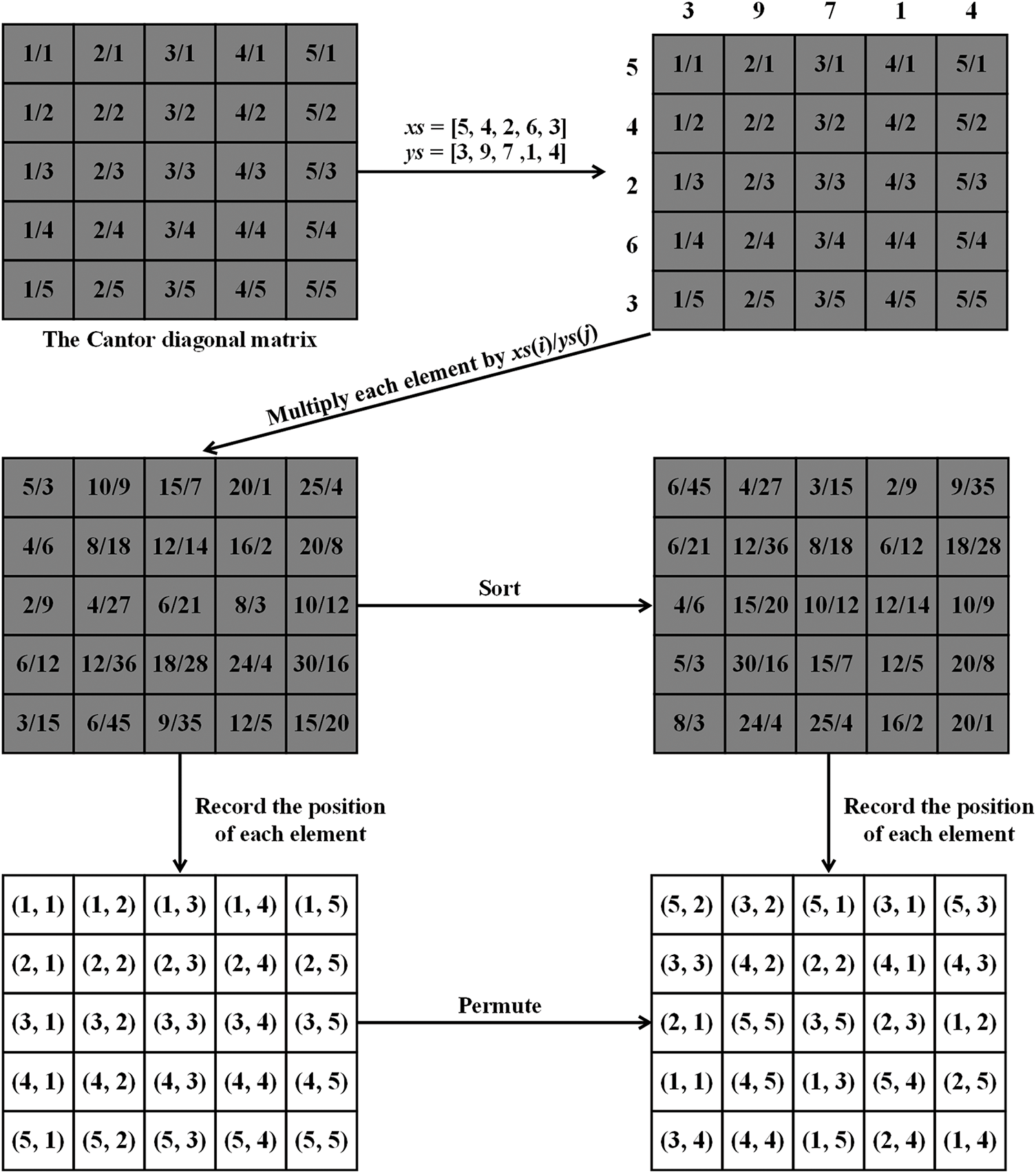
Figure 1: The Cantor diagonal matrix permutation process

Fig. 2a shows the plain Baboon image. Fig. 2b shows the Baboon image after one round of Cantor diagonal matrix permutation. It can be observed from Fig. 2b that the permuted Baboon image exhibits no discernible outlines or patterns of the original image. Thus, no meaningful information about the plain Baboon can be gained from it.

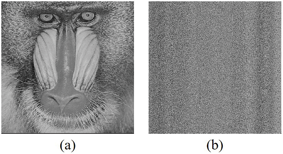
Figure 2: Cantor diagonal matrix permutation, (a) plain Baboon, (b) permuted Baboon

Fig. 3a–c, respectively displays the Baboon image after one round of Arnold permutation, Zigzag permutation, and Hilbert permutation. It can be observed from Fig. 3a that the permuted Baboon image using Arnold permutation still reveals the approximate outline of the original plain image. Fig. 3b,c shows that the images permuted by Zigzag and Hilbert methods exhibit distinct textures. Furthermore, Arnold permutation, Zigzag permutation, and Hilbert permutation are only applicable to square images, and Arnold permutation possesses periodicity. In contrast, Cantor diagonal matrix permutation can encrypt images of arbitrary sizes, achieving good results with just a single round of permutation.

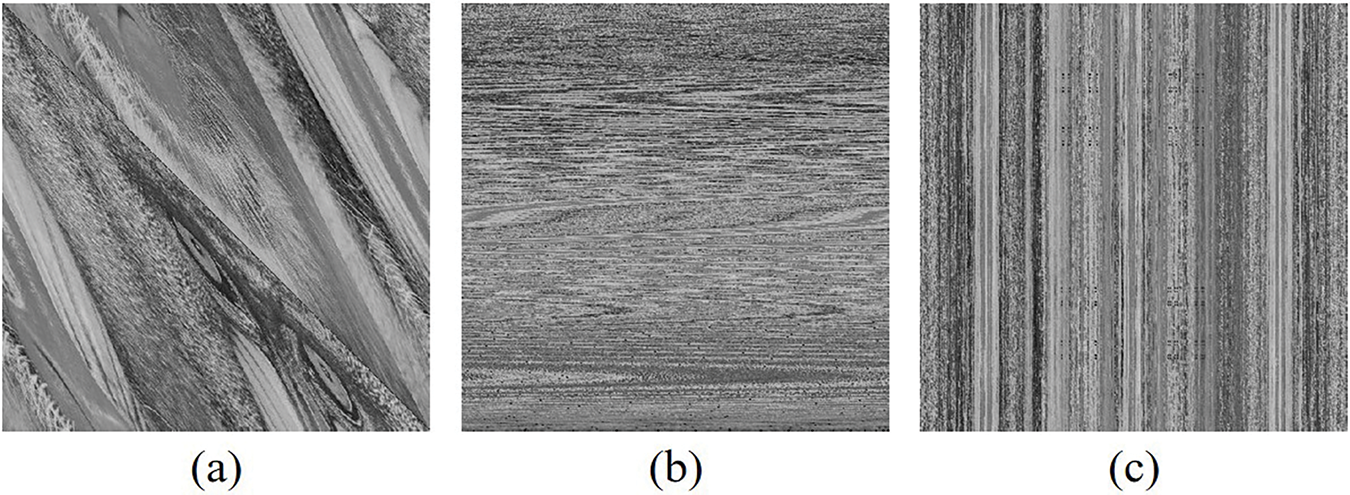
Figure 3: Permutation comparisons, (a) Arnold permutation, (b) Zigzag permutation, (c) Hilbert permutation

Correlation analysis examines the association between two or more variables to quantify their degree of association [16]. The correlation coefficient r, which measures this relationship, is mathematically expressed in Eq. (1).

{E(x)=1N∑i=1NxiD(x)=1N∑i=1N(xi−E(x))2cov(x,y)=1N∑i=1N(xi−E(x))(yi−E(y))rxy=cov(x,y)D(x)D(y).(1)

The range of r is [0, 1], with higher values indicating stronger pixel correlation. x and y are neighboring image pixels. We compared the adjacent pixel correlation coefficients in the horizontal (H), vertical (V), and diagonal (D) directions for the results of the proposed Cantor diagonal matrix permutation, Arnold permutation, Zigzag permutation, and Hilbert permutation. The results are listed in Table 1. Thus, the proposed Cantor diagonal matrix permutation demonstrates lower correlation coefficients than other permutation algorithms, indicating its effectiveness and security.

3  Chaotic Fractal Matrix

Fractal theory is an important branch of mathematics and geometry, focusing on the study of geometric patterns with self-similarity. Self-similarity refers to the property where an object exhibits complete or nearly identical resemblance to a portion of itself. Fractals are widely observed in nature, science, and artistic domains. The fundamental principle of fractal theory lies in generating infinitely complex structures through simple iterative rules. This paper integrates fractal theory with matrix theory to establish the concept of fractal matrices [21]. A matrix is classified as a fractal matrix when it satisfies three key characteristics. First, its element arrangement exhibits inherent self-similarity at different scales. Second, the matrix can be produced through iteration generation processes. Third, through limitless iterative steps, the matrix can theoretically expand without bound while maintaining its fundamental properties.

The chaotic fractal matrix is a novel concept combining fractal matrices and chaotic systems. As chaotic systems exhibit pseudo-random behavior, sensitivity to initial conditions, and parameter sensitivity, they are employed to control the starting values of the chaotic fractal matrix. Specifically, the chaotic fractal matrix is iteratively generated using initial parameters a, b, c, d, variable e, governed by the chaotic system, along with M and N. M indicates the image row count, and N denotes the column count. The subsequent Algorithm 1 delineates the methodology for constructing the chaotic fractal matrix FM:

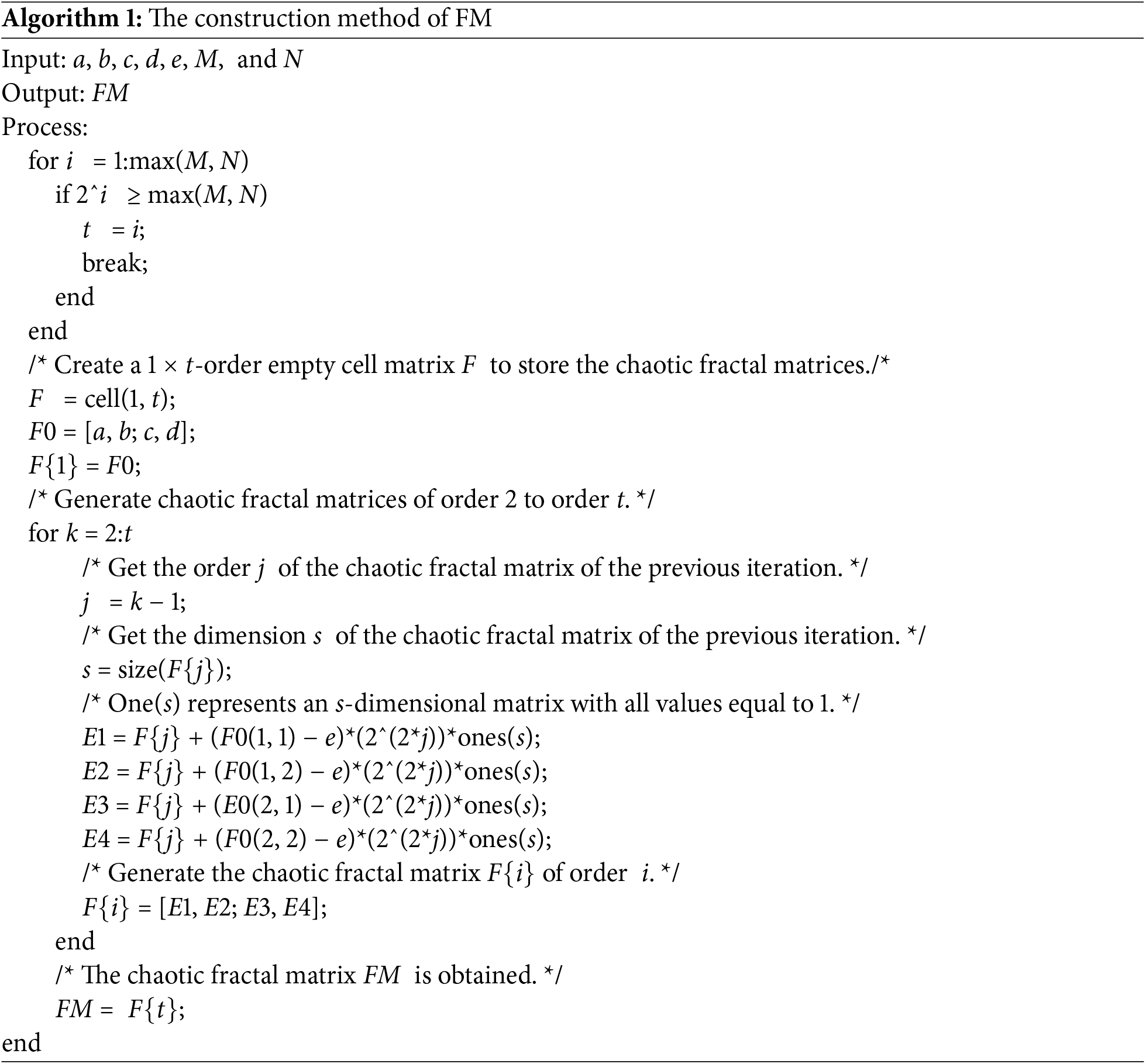
First, calculate the order t of the chaotic fractal matrix FM based on the image dimensions. Then, use the values a, b, c, and d generated by the chaotic system as initial values to construct the matrix of order 1. Finally, recursively construct matrices from order 2 to order t. Here, e is a variable. For each order k, the matrix consists of four sub-blocks. These sub-blocks are obtained by adding an offset to the matrix of order k − 1. To illustrate the concept of a chaotic fractal matrix, we present an exemplar in Fig. 4. Let a = 0.3, b = 0.1, c = 0.2, d = 0.4, e = 0.1, m = 3 and n = 4. The chaotic fractal matrix FM is generated through iteration. Arrange the four FM sub-blocks sequentially and annotate the sorted sequence with distinct red numerals. Notably, the element arrangement within each sub-block mirrors that of F1.

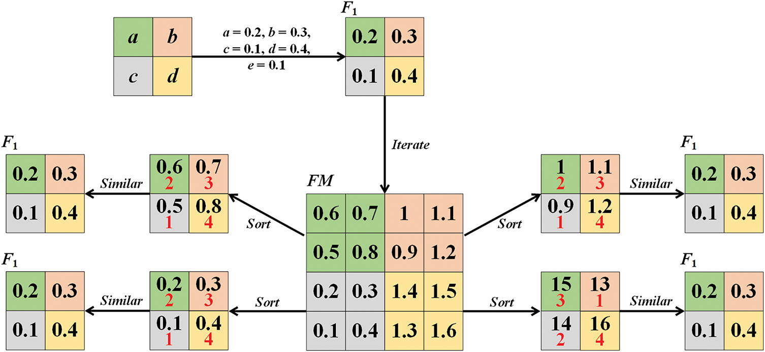
Figure 4: The chaotic fractal matrix

4  Encryption Algorithm

This section presents encryption and decryption methods using the Cantor diagonal matrix and chaotic fractal matrix, along with an associated chaotic system.

4.1 CML System

The spatiotemporal chaotic system has complex and excellent dynamic characteristics, so it is widely used in encryption schemes. This paper employs the CML system to generate chaotic sequences [17], which enables the proposed algorithm to have excellent performance and good security. The CML system is described as:

{xn+1(i)=(1−e)f[xn(i)]+e2{f[xn(i+1)]+f[xn(i−1)]}f(xn)=μxn(1−xn).(2)

In Eq. (2), the variable i denotes the lattice (i = 1 to L). L denotes the overall lattice count in the CML. The variable n serves as the time marker (n = 1, 2, 3…). The adjacent lattices to i are i + 1 and i − 1. When i = 1, i − 1 = L; when i = L, i + 1 = 1. e and μ are the parameters of CML. 0 ≤ e ≤1, 0 < μ ≤ 4 and 0 < f(x) < 1. When 3.57 ≤ μ ≤ 4, f(x) is in chaos. Lyapunov exponents characterize the dynamic behavior of chaotic systems [5]. When a Lyapunov exponent is greater than zero, the system is in a chaotic state. CML can be viewed as an L-dimensional system, where each lattice is equivalent to a chaotic system. Consequently, each lattice has its own Lyapunov exponent. The Kolmogorov-Sinai entropy density (h) and the Kolmogorov-Sinai entropy breadth (hu) are normalizations of the Lyapunov exponents. In Ref. [9], h represents the average of the positive Lyapunov exponents across the L lattices. hu denotes the percentage of lattices possessing positive Lyapunov exponents. Larger values of h and hu indicate stronger chaotic behavior in the CML. Fig. 5 shows the h and hu of the CML. Clearly, when μ > 3.8 and e > 0.2, all lattices exhibit good chaotic behavior. When the CML is in chaos, L chaotic sequences can be generated at the same time. In addition, the CML system boasts good randomness, extensive parameter space, and wide selection of initial conditions. Therefore, the suggested algorithm uses the CML system to generate chaotic sequences.

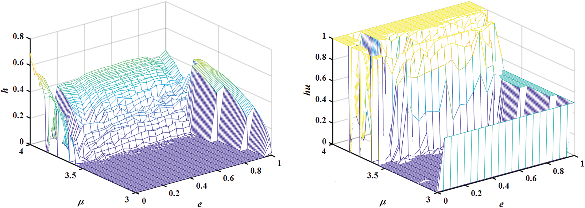
Figure 5: Kolmogorov-Sinai entropy

4.2 The Encryption Process

Input: An image P; with key K, 320-bit length.

Step 1: Split K into 8 equal parts (k1, k2, ..., k8). Convert these parts into the coefficients and initial values of the six lattices of CML, as shown in Eq. (3).

{x0(j)=∑i=140kj(i)×2i−1240,(j=1 to 6)e=∑i=140k7(i)×2i−1240μ=3.999+0.001×∑i=140k8(i)×2i−1240.(3)

Step 2: Input μ, e, and x0(j) (j = 1 to 6) into CML, then iterate M × N + 500 times to generate six sequences (cs1, cs2, cs3, cs4, cs5, cs6). The last five iterations from the first lattice serve as the variables and initial conditions for the chaotic fractal matrix FM1. Similarly, the last five iterations from the second lattice serve as the variables and initial conditions for the chaotic fractal matrix FM2. Use Eq. (4) to get d1, d2, d3, and d4. Extract values from iterations 500 to M + 500 of the fifth lattice for xs(i) (i = 1 to M). Extract values from iterations 500 to N + 500 of the sixth lattice for ys(j) (j = 1 to N).

{d1=floor[cs3(M×N)×1010]mod256d2=floor[cs3(M×N+500)×1010]mod256d3=floor[cs4(M×N)×1010]mod256d4=floor[cs4(M×N+500)×1010]mod256.(4)

Step 3: Compute FM1 and FM2 from the variables and initial conditions; details are outlined in Section 3.

Step 4: Apply diffusion I to P to derive semi-ciphertext S, where T = M × N. The specifics are outlined in Eq. (5).

{S(1)={P(1)+FM1(1)+floor [103×3.999×3.999×(d1/255)×(1−d1/255)×(1−3.999×(d1/255)×(1−d1/255))]+d2}mod256S(2)={P(2)+FM1(2)+floor [103×3.999×3.999×(d2/255)×(1−d2/255)×(1−3.999×(d2/255)×(1−d2/255))]+S(1)}mod256S(i)={P(i)+FM1(i)+floor [103×3.999×3.999×(S(i−2)/255)×(1−S(i−2)/255)×(1−3.999×(S(i−2)/255)×(1−S(i−2)/255))]+S(i−1)}mod256,i=3 to T.(5)

Step 5: Apply Cantor diagonal matrix permutation to S to derive the semi-ciphertext E; details are outlined in Section 2.

Step 6: Apply diffusion II to E to derive ciphered image F. The detailed procedure is detailed in Eq. (6).

{F(1)={E(1)+FM2(1)+floor [103×3.999×3.999×(d3/255)×(1−d3/255)×(1−3.999×(d3/255)×(1−d3/255))]+d4}mod256F(2)={E(2)+FM2(2)+floor [103×3.999×3.999×(d4/255)×(1−d4/255)×(1−3.999×(d4/255)×(1−d4/255))]+F(1)}mod256F(i)={E(i)+FM2(i)+floor [103×3.999×3.999×(F(i−2)/255)×(1−F(i−2)/255)×(1−3.999×(F(i−2)/255)×(1−F(i−2)/255))]+F(i−1)}mod256,i=3 to T.(6)

Output: F.

Fig. 6 depicts the encryption process. The proposed algorithm incorporates two diffusion operations and one permutation operation. First, the initial values and parameters for the four lattices of the CML system are generated from the secret key K. The CML system is then iterated to generate the parameters and sequences required for the permutation and diffusion processes, as well as the initial values and variables for two chaotic fractal matrices. Two chaotic fractal matrices are generated according to their construction algorithm for use in the two diffusion operations. The plain image P undergoes Diffusion I to obtain the semi-ciphertext image S. The semi-ciphertext image S is then permuted using Cantor diagonal matrix permutation to produce the semi-ciphertext image E. Finally, the semi-ciphertext image E undergoes Diffusion II to yield the final ciphered image F.

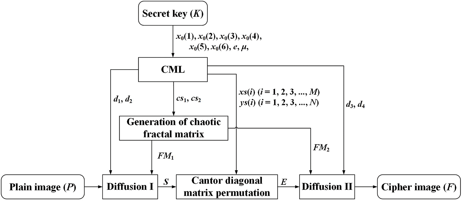
Figure 6: Encryption process

4.3 The Decryption Process

The algorithm suggested is both symmetric and invertible. Its decryption mirrors the encryption process in reverse. The detailed steps are:

Input: Ciphered image F; with key K, 320-bit length.

Step 1: Split K into 8 equal parts (k1, k2, ..., k8). Convert these parts into the coefficients and initial values of the six lattices of CML, as shown in Eq. (3).

Step2: Input μ, e, and x0(j) (j = 1 to 6) into CML, then iterate M × N + 500 times to generate six sequences (cs1, cs2, cs3, cs4, cs5, cs6). The last five iterations from the first lattice serve as the variables and initial conditions for the chaotic fractal matrix FM1. Similarly, the last five iterations from the second lattice serve as the variables and initial conditions for the chaotic fractal matrix FM2. Use Eq. (4) to get d1, d2, d3, and d4. Extract values from iterations 500 to M + 500 of the fifth lattice for xs(i) (i = 1 to M). Extract values from iterations 500 to N + 500 of the sixth lattice for ys(j) (j = 1 to N).

Step 3: Compute FM1 and FM2 from the variables and initial conditions; details are outlined in Section 3.

Step 4: Apply the reverse of diffusion II to F to derive E; details are outlined in Eq. (7).

{E(1)={F(1)−d4−floor [103×3.999×3.999×(d3/255)×(1−d3/255)×(1−3.999×(d3/255)×(1−d3/255))]−FM2(1)}mod256E(2)={F(2)−F(1)−floor [103×3.999×3.999×(d4/255)×(1−d4/255)×(1−3.999×(d4/255)×(1−d4/255))]−FM2(2)}mod256E(i)={F(i)−F(i−1)−floor [103×3.999×3.999×(F(i−2)/255)×(1−F(i−2)/255)×(1−3.999×(F(i−2)/255)×(1−F(i−2)/255))]−FM2(i)}mod256,i=3 to T.(7)

Step 5: Apply the reverse Cantor diagonal matrix permutation to E to derive S; details are provided in Section 2.

Step 6: Apply the reverse of diffusion I to S to obtain P, as detailed in Eq. (8).

{P(1)={S(1)−d2−floor [103×3.999×3.999×(d1/255)×(1−d1/255)×(1−3.999×(d1/255)×(1−d1/255))]−FM1(1)}mod256P(2)={S(2)−S(1)−floor [103×3.999×3.999×(d2/255)×(1−d2/255)×(1−3.999×(d2/255)×(1−d2/255))]−FM1(2)}mod256P(i)={S(i)−S(i−1)−floor [103×3.999×3.999×(S(i−2)/255)×(1−S(i−2)/255)×(1−3.999×(S(i−2)/255)×(1−S(i−2)/255))]−FM1(i)}mod256,i=3 to T.(8)

Output: P.

5  Simulation Experiments

The suggested algorithm was verified for performance using MATLAB. Images for the tests were acquired from the USC-SIPI database. Except for Kodim (768 × 512) and Hill (1024 × 1024), all other test images are 512 × 512 in size.

5.1 Experimental Results

Fig. 7 illustrates grayscale image encryption and decryption.

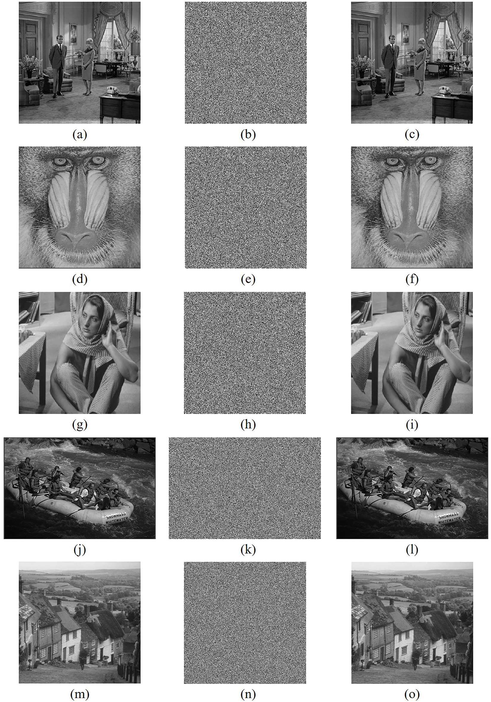
Figure 7: Simulation results of images, (a) Couple, (b) Ciphered image of Couple, (c) Decrypted image of Couple, (d) Baboon, (e) Ciphered image of Baboon, (f) Decrypted image of Baboon, (g) Barb, (h) Ciphered image of Barb, (i) Decrypted image of Barb, (j) Kodim (768 × 512), (k) Ciphered image of Kodim (768 × 512), (l) Decrypted image of Kodim (768 × 512), (m) Hill (1024 × 1024), (n) Ciphered image of Hill (1024 × 1024), (o) Decrypted image of Hill (1024 × 1024)

5.2 Pixel Spatial Distribution

Pixel spatial distribution in images serves as a key metric for evaluating encryption algorithm performance [16]. Fig. 8 illustrates the pixel spatial distributions of Couple, Baboon, and Barb, along with their corresponding ciphertexts. The plain images exhibit an irregular pixel distribution, marked by pronounced fluctuations between high and low concentrations (see Fig. 8a,c,e). This uneven spread suggests the presence of substantial meaningful data within the image. In contrast, the ciphered images demonstrate a far more uniform pixel distribution, effectively scrambling the plain images. As a result, the pixel values become evenly dispersed across the full [0, 255] range, as clearly visible in Fig. 8b,d,f.

Figure 8: Pixel spatial distribution of images, (a) Couple, (b) Ciphered image of Couple, (c) Baboon, (d) Ciphered image of Baboon, (e) Barb, (f) Ciphered image of Barb

The histogram depicts the occurrence of each grayscale level and illustrates pixel distribution. Fig. 9 displays the histograms of the plain images (Couple, Baboon, and Barb) alongside their ciphered images. The plain image histograms show uneven distributions, with sharp peaks and troughs indicating pixel intensity fluctuations. In contrast, an effective encryption algorithm should produce ciphered images with nearly uniform histograms, as demonstrated in Fig. 9b,d,f. These ciphered histograms show balanced grayscale distributions, where pixel values occur with roughly equal frequency. This uniformity makes statistical analysis impractical for potential attackers, significantly enhancing encryption security.

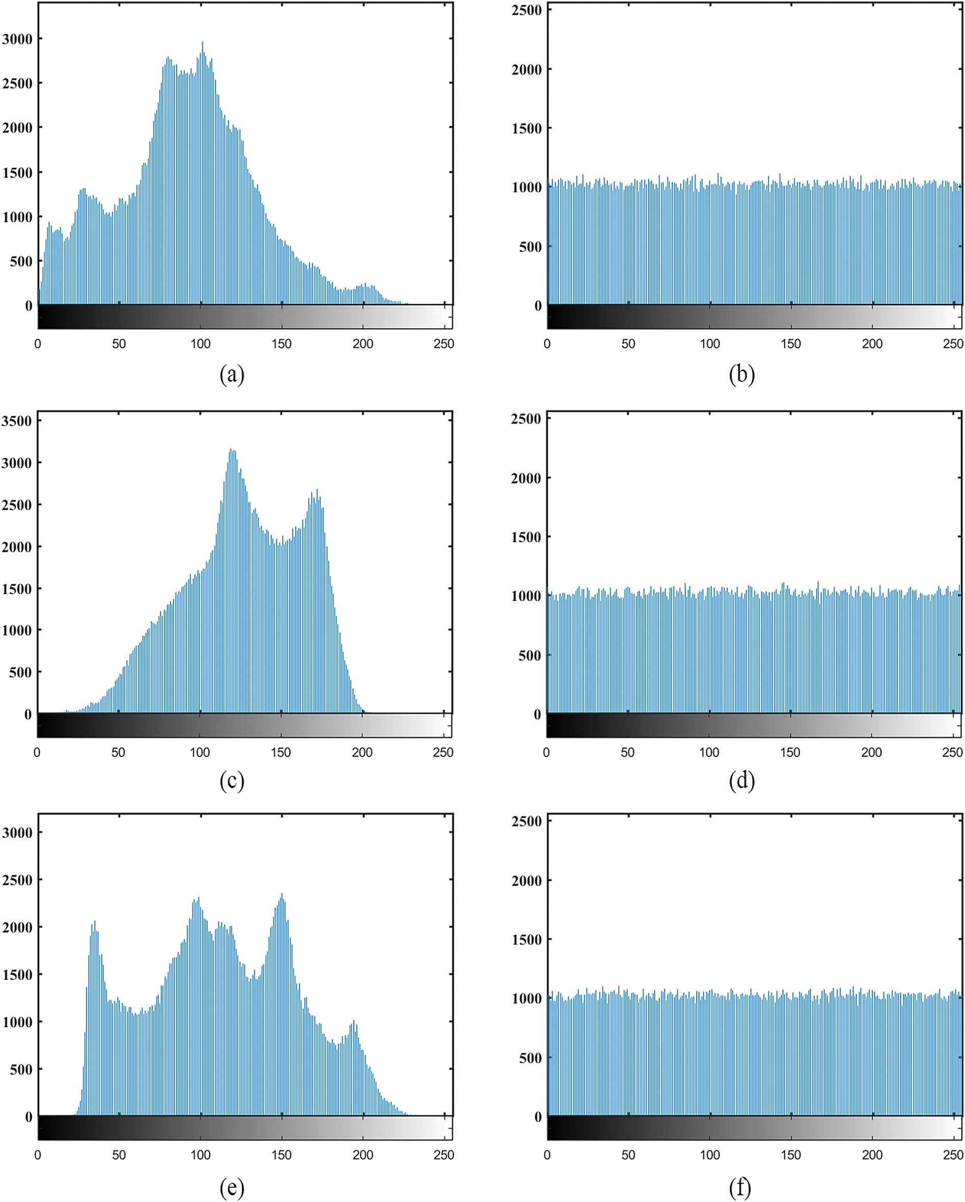
Figure 9: Histogram analysis for images, (a) Couple, (b) Ciphered image of Couple, (c) Baboon, (d) Ciphered image of Baboon, (e) Barb, (f) Ciphered image of Barb

The polar histogram serves as a crucial metric for evaluating encryption effectiveness [23]. The polar histogram of a plain image exhibits an irregular profile, typically characterized by large fluctuations in radial values across different angles and distinct peaks. This indicates the presence of regions with similar grayscale values within the plain image. Under ideal conditions, the polar histogram of a ciphered image should demonstrate a uniform distribution, with minimal fluctuations in radial values across all angles and no discernible peaks. This signifies that the encryption process randomizes pixel intensities, altering the distribution characteristics of the plain image and causing the statistical properties of the image to tend towards consistency across all angles.

As shown in Fig. 10, the polar histogram of the ciphered images approaches a stationary distribution, displaying no significant peaks at any angle. This indicates that the proposed algorithm uniformly distributes the plaintext pixels across the entire range. Consequently, it becomes difficult to recover the original content from the encrypted image through statistical analysis, thus demonstrating the effectiveness of the proposed algorithm.

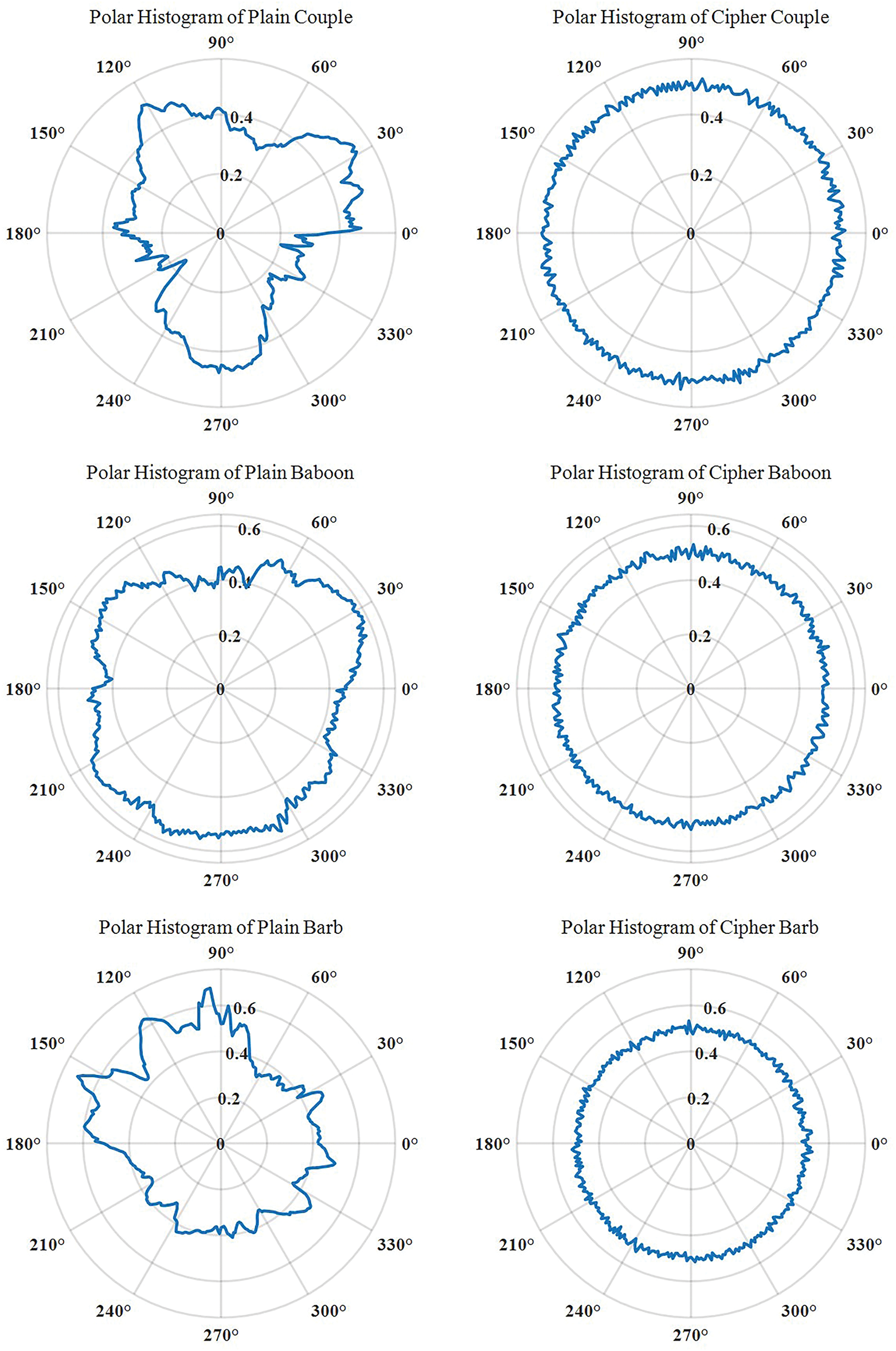
Figure 10: Polar histogram analysis

5.3 Information Entropy

Information entropy (IE) serves as a crucial measure for assessing the degree of information randomness [8], expressed as:

IE(S)=∑i=02N−1p(si)log2⁡1p(si).(9)

In Eq. (9), s denotes the image, while si refers to an individual pixel within S, and p(si) denotes the frequency of occurrence for si. Consequently, the upper limit for IE is 8. As IE approaches this maximum, the pixel distribution becomes increasingly uniform. Table 2 presents the IE of Couple, Baboon, Barb, Boat, and Airplane, along with their ciphered counterparts. As can be seen, each ciphered image boasts an entropy well over 7.997, nearing the ideal value. Compared to other schemes, the proposed method in this paper exhibits a higher information entropy, thereby ensuring enhanced security.

Ref. [28] states that local information entropy (LE) quantifies pixel distribution randomness, defined as:

LEk,TB(S)¯=∑i=1kIE(Si)k.(10)

In Eq. (10), Si denotes k random subsets of TB pixels selected from the image. while IE(Si) corresponds to their IE. According to Ref. [28], with a confidence level α of 0.01, k set to 30, and TB fixed at 1936, the expected range for LE falls between 7.9017 and 7.9032. As illustrated in Table 3, the calculated LE values for the ciphered images of Couple, Baboon, Barb, Boat and Airplane all lie within this interval, confirming their compliance with the test criteria.

5.4 Differential Attack

Differential attack is a chosen-plaintext attack method targeting symmetric encryption algorithms. A robust encryption algorithm typically exhibits strong resistance to differential attack, a quality often referred to as plaintext sensitivity in cryptographic circles [14]. Plaintext sensitivity is quantified by comparing ciphertexts from similar images encrypted with identical keys. This difference is characterized by the NPCR (number of pixels change rate) and UACI (unified average changing intensity), as detailed in Eq. (11).

{NPCR=∑i,jD(i,j)C×R×100%UACI=1C×R[∑i,j|f1(i,j)−f2(i,j)|255]×100%.(11)

Here, f1 and f2 represent the two ciphered images, while C and R denote their width and height, respectively. The expected NPCR benchmark is 99.6094%, and the ideal UACI threshold stands at 33.4635%. For testing, five plain images are used. A single pixel in each image is incremented by 1, followed by NPCR and UACI computation. Table 4 provides the NPCR and UACI metrics for ciphertexts and computes their respective averages. Table 5 contrasts these results with those from other algorithms. As depicted in Table 4, the NPCR and UACI for the test images are notably close to the standard values, indicating that even minor alterations in pixel values significantly impact the entire encrypted image.

5.5 Key Space

The key space size of an algorithm dictates its brute-force attack resistance. An effective encryption algorithm requires an adequately expansive key space. In the suggested algorithm, the 320-bit key ensures a vast key space of 2320, providing strong resistance to brute-force attacks.

5.6 Key Sensitivity Analysis

The sensitivity of the secret key is a crucial factor in evaluating the performance of encryption algorithms [8]. In the event that a single parameter of the decryption key varies slightly from the actual secret key, and the resulting decrypted image bears no resemblance to the original, it indicates a high level of sensitivity to the secret key within the scheme. The suggested scheme utilizes a 320-bit key, which is then evenly split into eight sub-keys, serving as the initial value for CML along with the coefficients e and μ. To rigorously assess the sensitivity of the key, we modified it in three distinct scenarios, flipping just one bit at a time in each case. Fig. 11a displays the original Couple image. Without loss of generality, the encryption key K is modified by flipping either the 113th, 261st, or 297th bit, generating three altered keys: K1, K2 and K3. These modified keys are then used to decrypt the ciphered Couple, producing the corresponding decrypted images P1, P2 and P3 (illustrated in Fig. 11b–d). As evident from the results, the decrypted images exhibit completely randomized pixel distributions, bearing no resemblance to the original image or revealing any meaningful visual data. Thus, the suggested algorithm is highly sensitive to secret key variations.

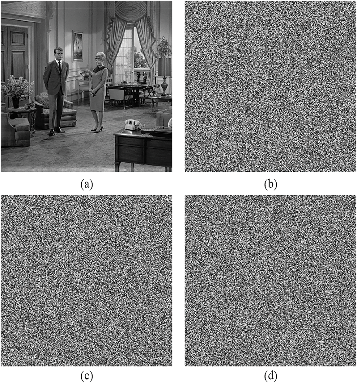
Figure 11: Secret key sensitivity analysis, (a) Couple, (b) P1, (c) P2, (d) P3

5.7 Correlation Analysis

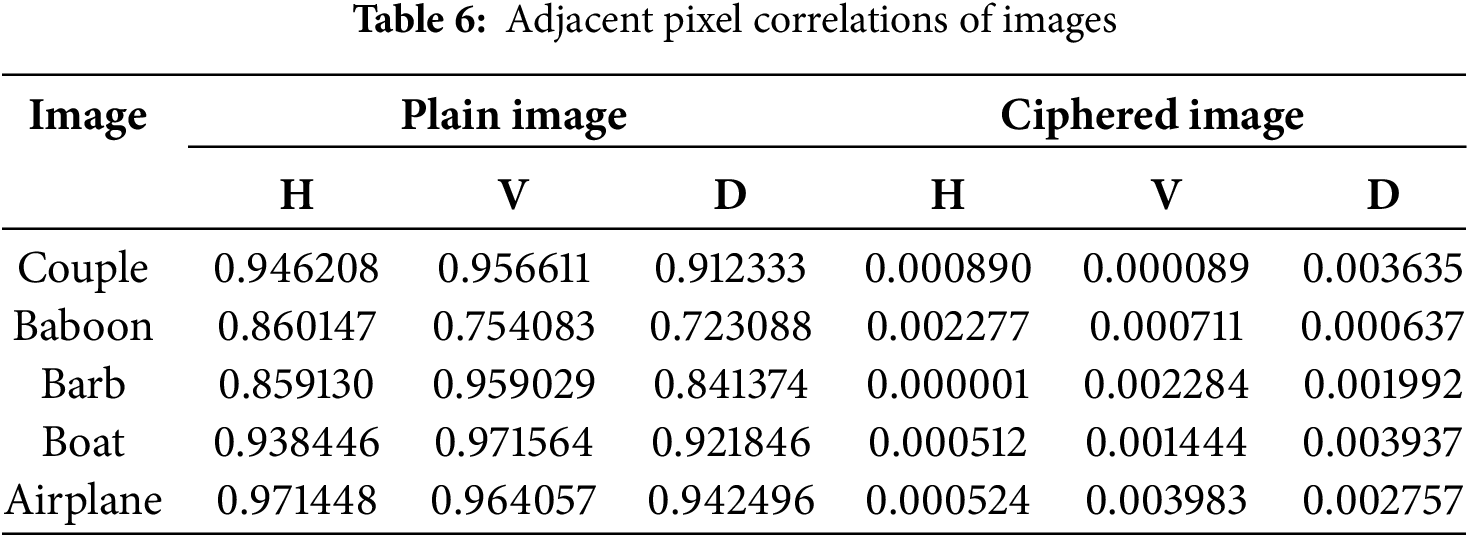
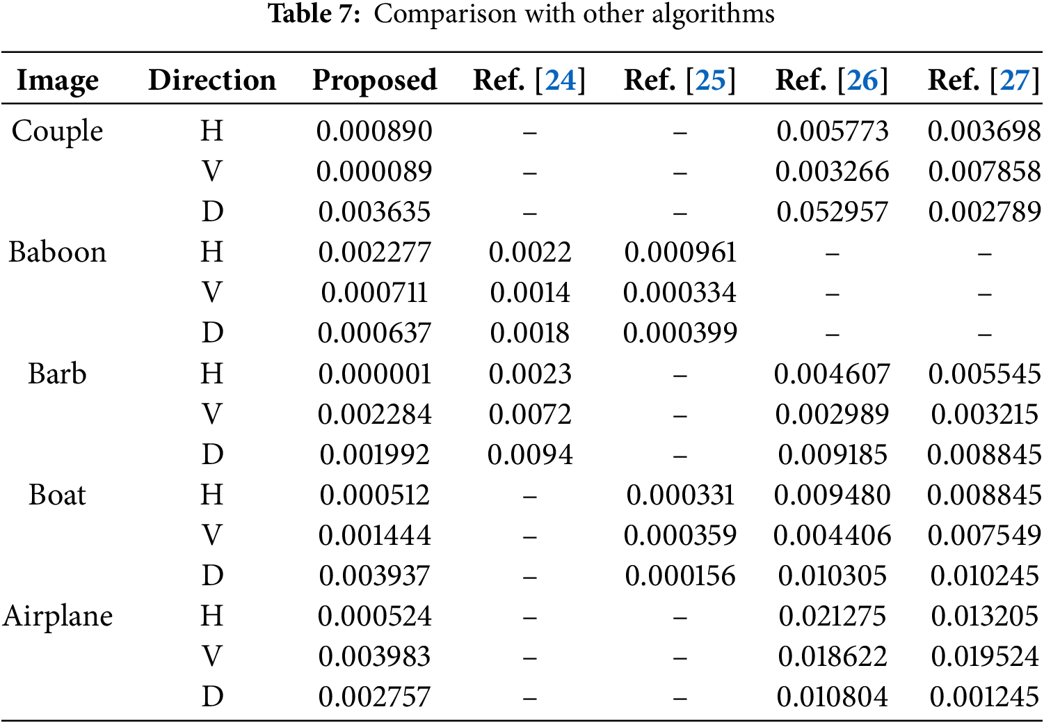
In the context of image processing, the correlation between neighboring pixels serves as an indicator of pixel diffusion. Plain images typically exhibit strong correlations among adjacent pixels, whereas properly ciphered images should display near-zero correlation. The correlation coefficient r is defined in Eq. (1). Fig. 12 illustrates the correlation between neighboring pixels in both the plain and ciphered versions of the Couple across horizontal (H), vertical (V), and diagonal (D) axes. The findings indicate that the pixels within the ciphered image are more dispersed throughout. Table 6 presents the correlation coefficients between the plain images (Couple, Baboon, Barb, Boat, and Airplane) and their ciphered counterparts. Table 7 provides a comparative analysis with alternative encryption methods. While the plain images exhibit correlation coefficients approaching unity, indicating strong linear relationships, the ciphered images demonstrate a substantial decrease in these values, reflecting the effectiveness of the encryption process.

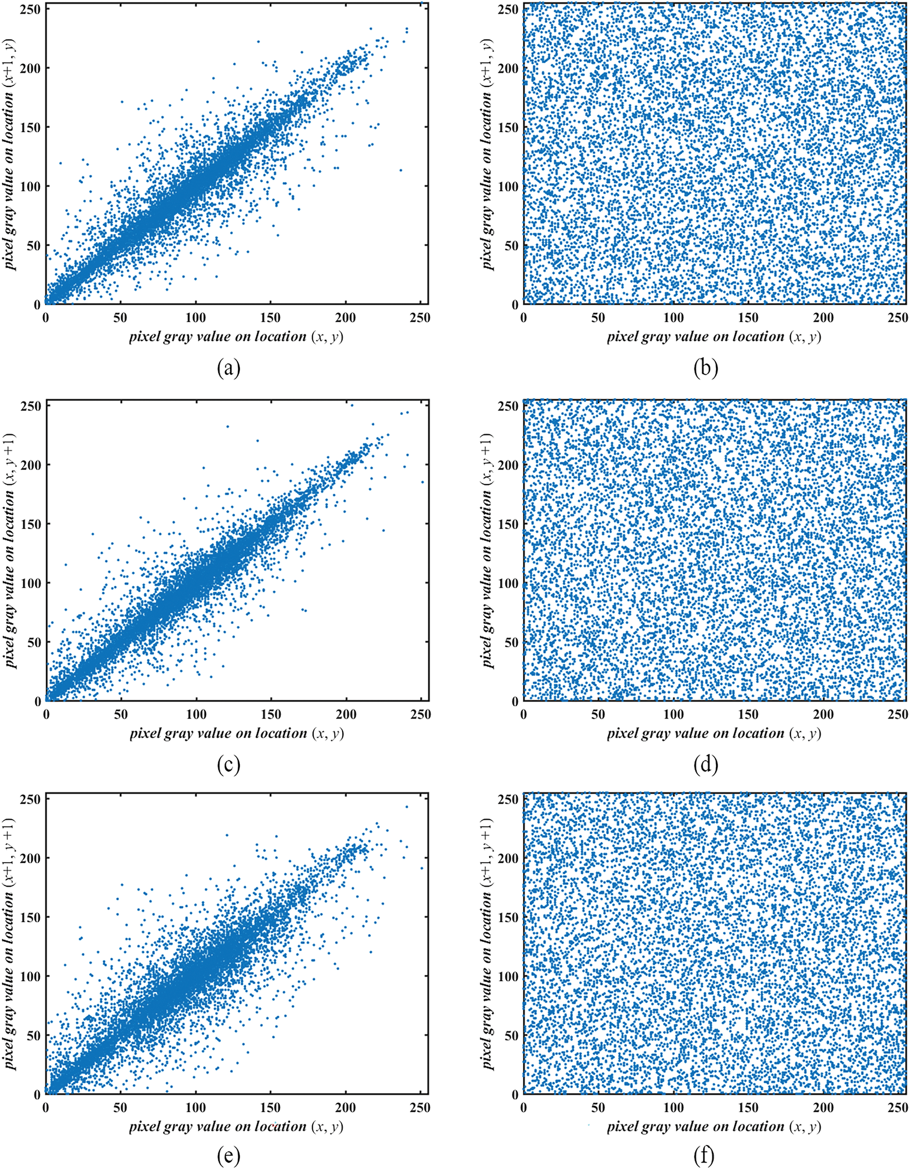
Figure 12: Adjacent pixels correlation, (a) H of Couple, (b) H of ciphered Couple, (c) V of Couple, (d) V of ciphered Couple, (e) D of Couple, (f) D of ciphered Couple

5.8 χ2 Test

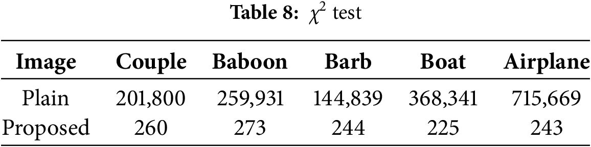
χ2 statistically represents the extent of pixel distribution variance from a completely even distribution. The definition is provided in Eq. (12).

χ2=∑i=0255(pi−p¯)2p¯.(12)

pi denotes the occurrence rate of pixel i within the image. The variable p¯ stands for the mean frequency across all pixels, computed as (r × c)/256, where r and c correspond to the height and width of images, respectively.

A lower χ2 value indicates a more uniform distribution of pixels. As illustrated in Table 8, the χ2 measurements for the plain images (Couple, Baboon, Barb, Boat, and Airplane) are substantially higher than those of their ciphered counterparts, demonstrating that the cipher process results in a far more balanced pixel distribution.

5.9 Floating Frequency Analysis

Floating frequency analysis is an intuitive and effective local statistical test method specifically designed for evaluating the performance of image encryption algorithms. It quantifies the randomness and uniformity of encryption results in both row and column directions by measuring the number of distinct pixel values and their spatial distribution within fixed-size windows. For a 256 × 256 grayscale image, the Column Floating Frequency (CFF) and Row Floating Frequency (RFF) are calculated as follows [23]:

1.    For each column, select a window containing 256 pixels. Calculate the number of distinct pixel values within this window to obtain the CFF for that column.

2.    For each row, select a window containing 256 pixels. Calculate the number of distinct pixel values within this window to obtain the RFF for that row.

3.    Compute the average values of CFF and RFF separately and plot their distributions.

For a 512 × 512 grayscale image: Each column is divided into two upper and lower windows of 256 pixels. The floating frequency of each window is calculated, and the average of the two windows is taken as the CFF for that column. Each row is divided into two left and right windows of 256 pixels. The floating frequency of each window is calculated, and the average of the two windows is taken as the RFF for that row.

Fig. 13 displays the floating frequencies of 512 × 512 plain images and their corresponding ciphered images, along with their average CFF and RFF values. The results show that the CFF and RFF of plain images are unevenly distributed with obvious peaks and valleys, and the average CFF and RFF are low. In contrast, the CFF and RFF of ciphered images are evenly distributed, significantly higher than those of the plain images, and both average values are greater than 161. Higher and more uniformly distributed CFF and RFF values indicate stronger spatial randomness generation capability of the encryption algorithm. Notably, if certain row or column regions of the ciphered image exhibit CFF or RFF values significantly below the average, this indicates insufficient encryption strength in those regions, where pixel value variations lack randomness. Such weaknesses may serve as potential entry points for cryptanalysis.

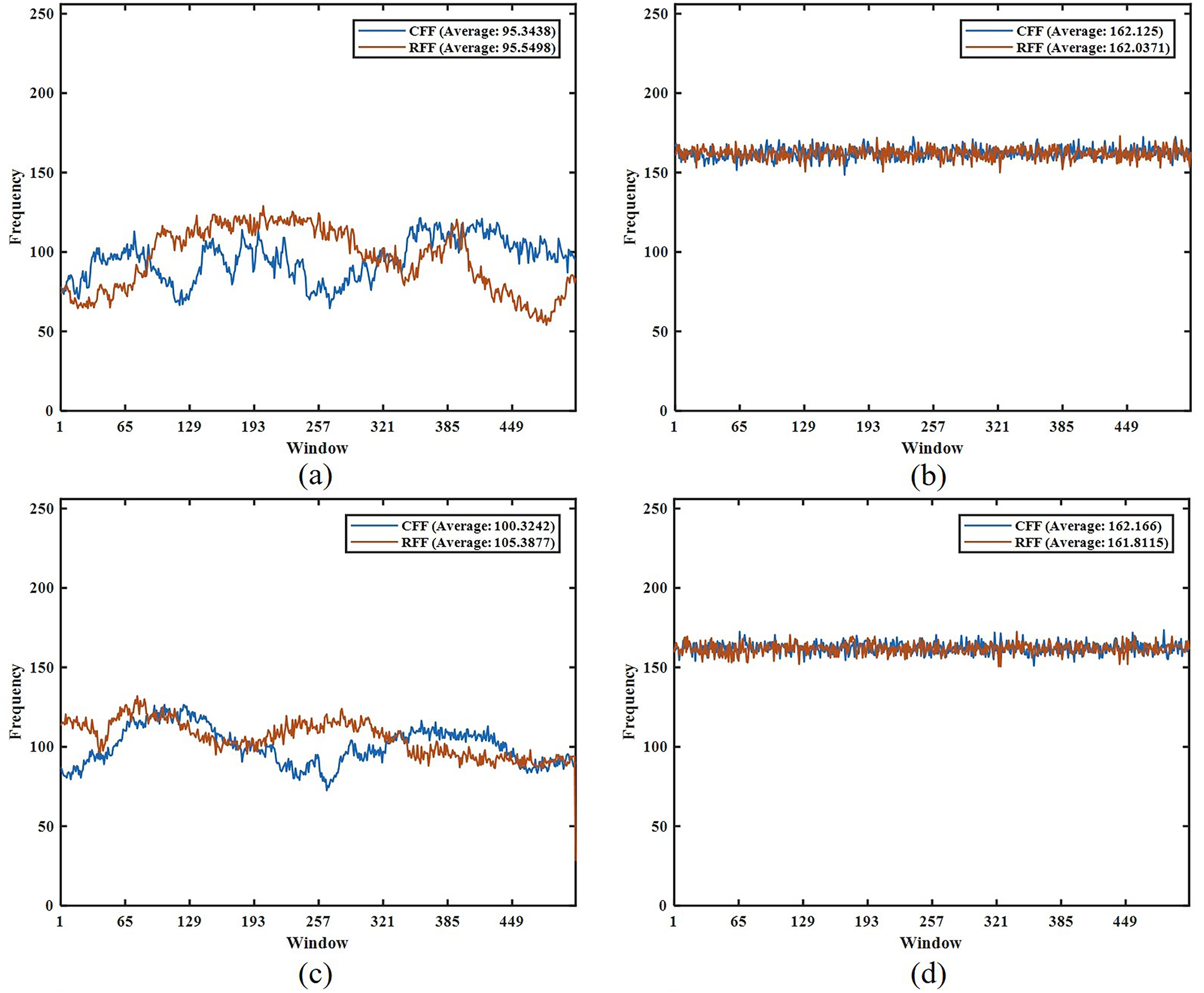
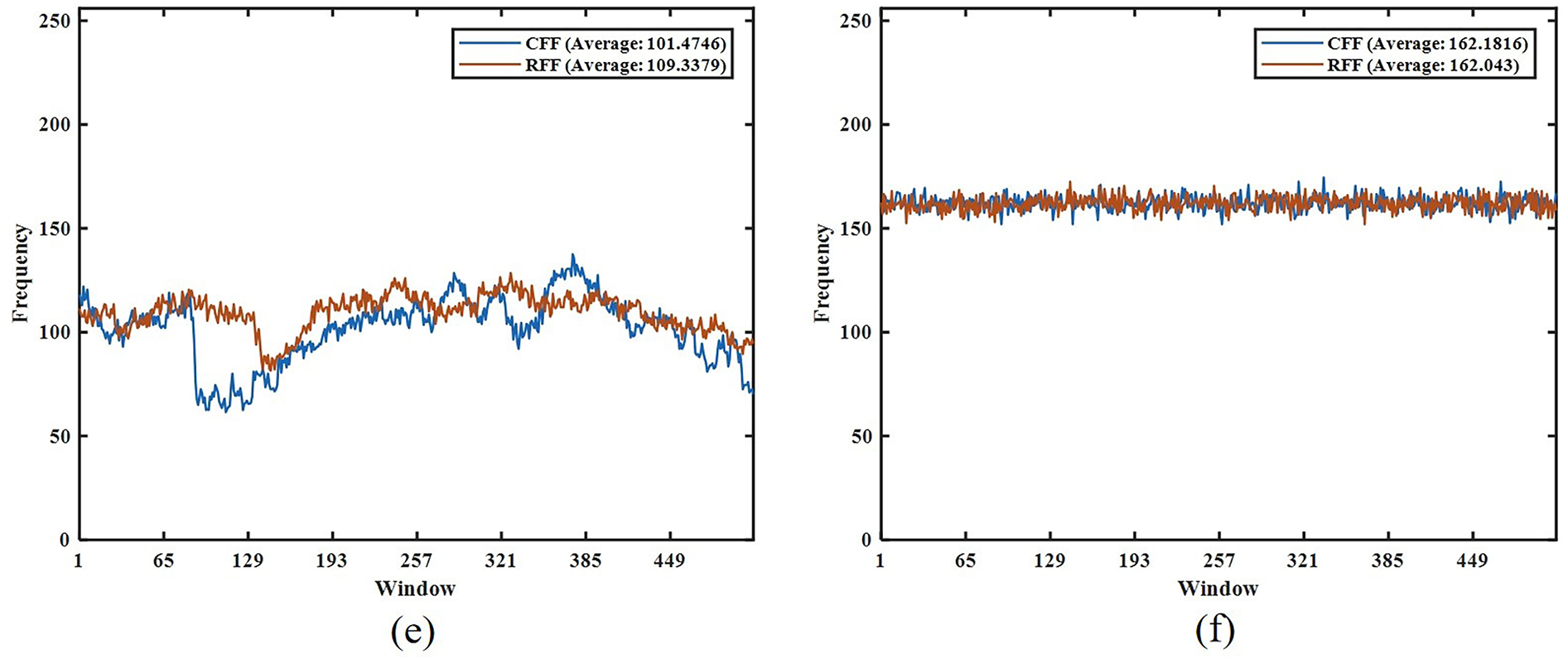
Figure 13: Floating frequency analysis, (a) Couple, (b) Ciphered image of Couple, (c) Baboon, (d) Ciphered image of Baboon, (e) Barb, (f) Ciphered image of Barb

5.10 Speed Performance

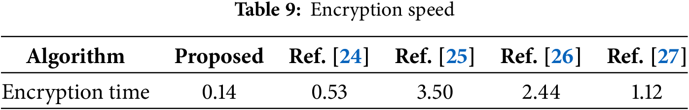
Encryption speed, a key performance metric for algorithms, is influenced by their design and the underlying hardware and software. The suggested scheme in question was executed in MATLAB 7 on a personal computer running Windows 10. The hardware specifications were an Intel(R) Core(TM) i7-9750H CPU clocked at 2.60 GHz, and boasting 16.0 GB of RAM. To maintain consistency in our analysis, we conducted 50 encryption trials for each of five standard test images: Couple, Baboon, Barb, Boat, and Airplane. The average processing times were then computed and presented in Table 9. The data clearly demonstrates that our encryption method outperforms competing algorithms (such as those in [24–27]) with significantly faster processing speeds, showcasing its superior computational efficiency.

5.11 Time Complexity

Although encryption time can measure efficiency of algorithms, it is affected by factors such as computer configuration, operating system, programming language, and compiler optimization options. Time complexity removes the influence of these specific hardware and software environments, focusing only on characteristics of efficiency inherent in the algorithm logic itself. Time complexity approaches from an algorithmic perspective, describing how running time of algorithms increases as input size grows. It is not concrete running time, but describes efficiency of algorithms abstractly.

The proposed encryption algorithm consists of six steps (see Section 4.2). The time complexity of Step 1 is O(1). The time complexity of Step 2 is O(M × N). The time complexity of Step 3 is O(max(M, N)2). The time complexity of Step 4 is O(M × N). The time complexity of Step 5 is O(M × N × log(M × N)). The time complexity of Step 6 is O(M × N). Since the time complexity of the encryption algorithm is determined by the step with the highest time complexity, the overall time complexity of the proposed encryption algorithm is O(max(M, N)2 + M × N × log(M × N)).

5.12 Memory Footprint

Memory footprint is an important indicator for measuring encryption algorithms. It is defined as the total memory required for the algorithm to run, including inputs, outputs, intermediate variables, buffers, keys, lookup tables, etc. [29]. Memory footprint reflects the consumption of computer random access memory resources during algorithm execution. To provide a comprehensive analysis, taking a 512 × 512 size image as an example, we calculated the memory usage of each component involved in the encryption process, and the results are listed in Table 10.

The total memory footprint of the proposed algorithm is 2,842,144 Bytes ≈ 2.71 MB. Since the proposed algorithm is a symmetric encryption algorithm, the decryption process also consumes the same memory. Given the complexity of encryption algorithms and spatiotemporal chaotic systems, the total memory footprint of the proposed algorithm demonstrates the efficiency of the algorithm and reflects the feasibility of deploying the algorithm in systems with moderate memory capacity.

5.13 Robustness Analysis

During the data transfer phase, a ciphered image is vulnerable to malicious interference, which can corrupt portions of the file or introduce disruptive artifacts [30,31]. Thus, the algorithm must exhibit high robustness. This robustness can be assessed through simulations involving clipping and noise attacks [32]. Fig. 14a displays the ciphertext Couple following the introduction of salt-and-pepper noise at a 1% density. The corresponding decrypted result is shown in Fig. 14b. Fig. 15 shows the clipping attack experiment results. A clear observation reveals that the decrypted versions retain the majority of essential visual data despite these alterations.

Figure 14: Noise attack, (a) Ciphered Couple after adding noise, (b) decrypted of (a)

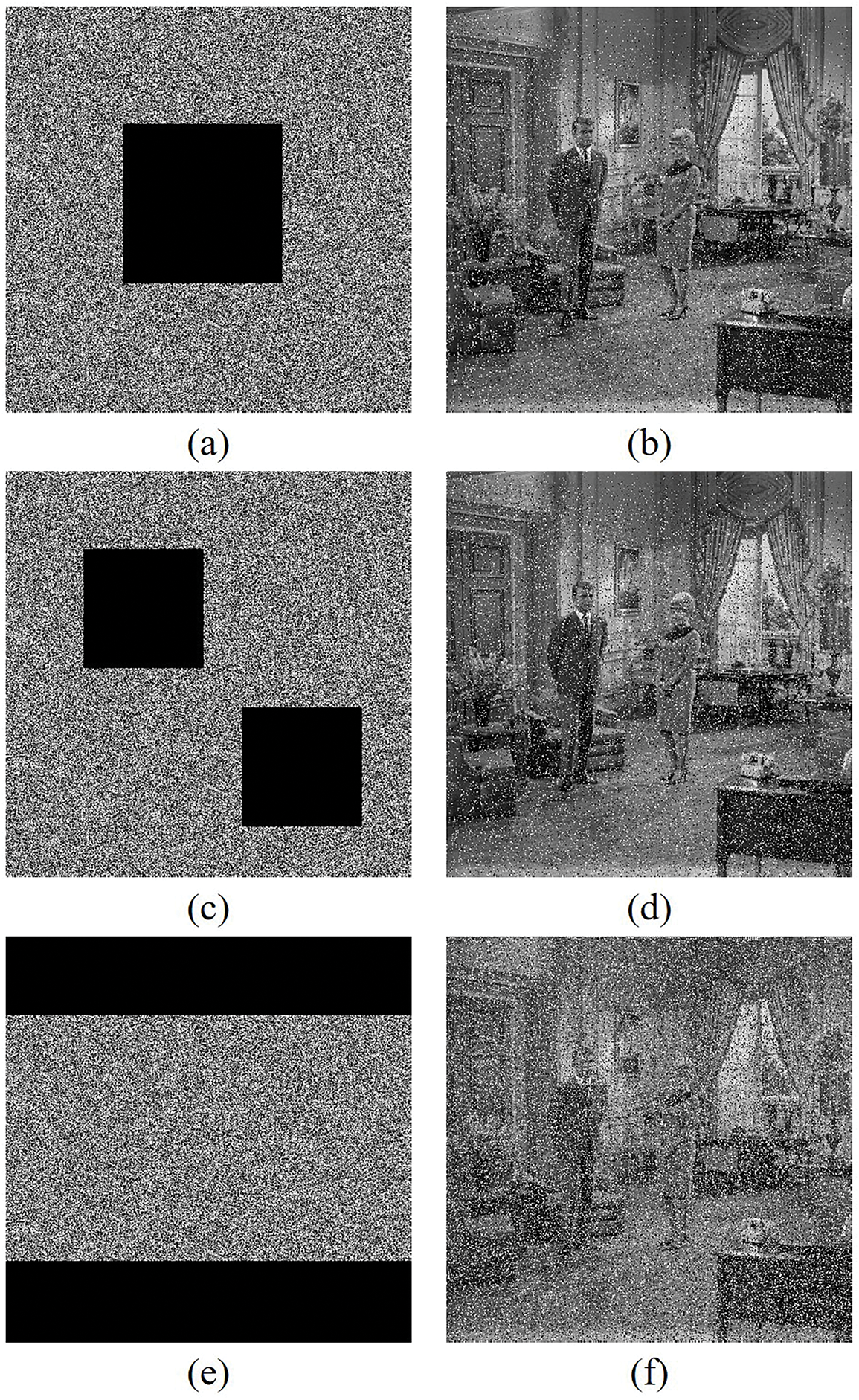
Figure 15: Clipping attack, (a) clipping 200 × 200 pixels, (b) decrypted of (a), (c) clipping 150 × 150 × 2 pixels, (d) decrypted of (c), (e) clipping 512 × 100 × 2 pixels, (f) decrypted of (e)

6  Conclusions

This paper introduces the Cantor diagonal matrix permutation technique along with chaotic fractal matrix. Subsequently, leveraging these concepts, the paper outlines a novel encryption algorithm. The suggested algorithm incorporates two diffusion steps, a single permutation step, and omits the need for iterative encryption rounds. Moreover, the proposed algorithm achieves exceptional performance with just a single round of encryption. In the end, extensive experimentation has fully confirmed its high security and robust statistical qualities. In future work, the algorithm will be refined and applied to additional data formats.

Acknowledgement: None.

Funding Statement: This work is supported by the National Natural Science Foundation of China (62376106), The Science and Technology Development Plan of Jilin Province (20250102212JC).

Author Contributions: The authors confirm contribution to the paper as follows: study conception and design: Hongyu Zhao, Shengsheng Wang; data collection: Hongyu Zhao, Shengsheng Wang; analysis and interpretation of result: Hongyu Zhao, Shengsheng Wang; draft manuscript preparation: Hongyu Zhao; supervision and funding acquisition: Shengsheng Wang. All authors reviewed the results and approved the final version of the manuscript.

Availability of Data and Materials: Data available on request from the authors.

Ethics Approval: Not applicable.

Conflicts of Interest: The authors declare no conflicts of interest to report regarding the present study.

References

1. Moses Setiadi DRI, Rijati N, Muslikh AR, Vicky Indriyono B, Sambas A. Secure image communication using Galois field, hyper 3D logistic map, and B92 quantum protocol. Comput Mater Continua. 2024;81(3):4435–63. doi:10.32604/cmc.2024.058478. [Google Scholar] [CrossRef]

2. Wang Y, Lei P, Yang H, Cao H. Security analysis on a color image encryption based on DNA encoding and chaos map. Comput Electr Eng. 2015;46:433–46. doi:10.1016/j.compeleceng.2015.03.011. [Google Scholar] [CrossRef]

3. Hua Z, Zhou Y, Huang H. Cosine-transform-based chaotic system for image encryption. Inf Sci. 2019;480(8):403–19. doi:10.1016/j.ins.2018.12.048. [Google Scholar] [CrossRef]

4. Dong Z, Zhang Z, Zhou H, Chen X. Color image compression and encryption algorithm based on 2D compressed sensing and hyperchaotic system. Comput Mater Continua. 2024;78(2):1977–93. doi:10.32604/cmc.2024.047233. [Google Scholar] [CrossRef]

5. He Y, Zhang YQ, He X, Wang XY. A new image encryption algorithm based on the OF-LSTMS and chaotic sequences. Sci Rep. 2021;11(1):6398. doi:10.1038/s41598-021-85377-1. [Google Scholar] [PubMed] [CrossRef]

6. Sun M, Yuan J, Li X, Liu D. Chaotic CS encryption: an efficient image encryption algorithm based on Chebyshev chaotic system and compressive sensing. Comput Mater Continua. 2024;79(2):2625–46. doi:10.32604/cmc.2024.050337. [Google Scholar] [CrossRef]

7. Zhang Y, He Y, Zhang J, Liu X. Multiple digital image encryption algorithm based on chaos algorithm. Mob Netw Appl. 2022;27(4):1349–58. doi:10.1007/s11036-022-01923-9. [Google Scholar] [CrossRef]

8. Zhang Y. The fast image encryption algorithm based on lifting scheme and chaos. Inf Sci. 2020;520(1):177–94. doi:10.1016/j.ins.2020.02.012. [Google Scholar] [CrossRef]

9. Zhao H, Wang S, Fu Z. A new image encryption algorithm based on cubic fractal matrix and L-LCCML system. Chaos Solitons Fractals. 2024;185(33–34):115076. doi:10.1016/j.chaos.2024.115076. [Google Scholar] [CrossRef]

10. Arab A, Rostami MJ, Ghavami B. An image encryption method based on chaos system and AES algorithm. J Supercomput. 2019;75(10):6663–82. doi:10.1007/s11227-019-02878-7. [Google Scholar] [CrossRef]

11. Song C, Qiao Y. A novel image encryption algorithm based on DNA encoding and spatiotemporal chaos. Entropy. 2015;17(10):6954–68. doi:10.3390/e17106954. [Google Scholar] [CrossRef]

12. Xiao S, Yu Z, Deng Y. Design and analysis of a novel chaos-based image encryption algorithm via switch control mechanism. Secur Commun Netw. 2020;2020:7913061. doi:10.1155/2020/7913061. [Google Scholar] [CrossRef]

13. Çavuşoğlu Ü, Kaçar S, Pehlivan I, Zengin A. Secure image encryption algorithm design using a novel chaos based S-Box. Chaos Solitons Fractals. 2017;95(11):92–101. doi:10.1016/j.chaos.2016.12.018. [Google Scholar] [CrossRef]

14. Zhang YQ, Wang XY, Liu J, Chi ZL. An image encryption scheme based on the MLNCML system using DNA sequences. Opt Lasers Eng. 2016;82(36):95–103. doi:10.1016/j.optlaseng.2016.02.002. [Google Scholar] [CrossRef]

15. Zhang H, Wang XQ, Wang XY, Yan PF. Novel multiple images encryption algorithm using CML system and DNA encoding. IET Image Process. 2020;14(3):518–29. doi:10.1049/iet-ipr.2019.0771. [Google Scholar] [CrossRef]

16. He Y, Zhang YQ, Wang XY. A new image encryption algorithm based on two-dimensional spatiotemporal chaotic system. Neural Comput Appl. 2020;32(1):247–60. doi:10.1007/s00521-018-3577-z. [Google Scholar] [CrossRef]

17. Kaneko K. Pattern dynamics in spatiotemporal chaos: pattern selection, diffusion of defect and pattern competition intermittency. Phys D Nonlinear Phenom. 1989;34(1–2):1–41. doi:10.1016/0167-2789(89)90227-3. [Google Scholar] [CrossRef]

18. Zhang YQ, Wang XY, Liu LY, He Y, Liu J. Spatiotemporal chaos of fractional order logistic equation in nonlinear coupled lattices. Commun Nonlinear Sci Numer Simul. 2017;52(4):52–61. doi:10.1016/j.cnsns.2017.04.021. [Google Scholar] [CrossRef]

19. Fan S, Chen K, Tian J. A novel image encryption algorithm based on coupled map lattices model. Multimed Tools Appl. 2024;83(4):11557–72. doi:10.1007/s11042-023-15964-z. [Google Scholar] [CrossRef]

20. Babinec P. Possible fractal structure of exact universal exchange-correlation potential. Chaos Solitons Fractals. 2004;22(5):1007–11. doi:10.1016/j.chaos.2004.04.007. [Google Scholar] [CrossRef]

21. Altun I, Sahin H, Aslantas M. A new approach to fractals via best proximity point. Chaos Solitons Fractals. 2021;146(1):110850. doi:10.1016/j.chaos.2021.110850. [Google Scholar] [CrossRef]

22. Wang X, Gao S, Ye X, Zhou S, Wang M. A new image encryption algorithm with cantor diagonal scrambling based on the PUMCML system. Int J Bifurcation Chaos. 2021;31(1):2150003. doi:10.1142/s0218127421500036. [Google Scholar] [CrossRef]

23. Iqbal N, Banga A, Innab N, ElZaghmouri BM, Ikram A, Diab H. Utilizing the nth root of numbers for novel random data Calculus and its applications in network security and image encryption. Expert Syst Appl. 2025;265(8):125992. doi:10.1016/j.eswa.2024.125992. [Google Scholar] [CrossRef]

24. Kumar S, Sharma D. Image scrambling encryption using chaotic map and genetic algorithm: a hybrid approach for enhanced security. Nonlinear Dyn. 2024;112(14):12537–64. doi:10.1007/s11071-024-09670-0. [Google Scholar] [CrossRef]

25. Farandi MNE, Marjuni A, Rijati N, Setiadi DRIM. Enhancing image encryption security through integration multi-chaotic systems and mixed pixel-bit level. Imag Sci J. 2025;73(3):363–80. doi:10.1080/13682199.2024.2398954. [Google Scholar] [CrossRef]

26. Farah MAB, Farah A, Farah T. An image encryption scheme based on a new hybrid chaotic map and optimized substitution box. Nonlinear Dyn. 2020;99(4):3041–64. doi:10.1007/s11071-019-05413-8. [Google Scholar] [CrossRef]

27. Farah MAB, Guesmi R, Kachouri A, Samet M. A new design of cryptosystem based on S-box and chaotic permutation. Multimed Tools Appl. 2020;79(27):19129–50. doi:10.1007/s11042-020-08718-8. [Google Scholar] [CrossRef]

28. Wu Y, Zhou Y, Saveriades G, Agaian S, Noonan JP, Natarajan P. Local Shannon entropy measure with statistical tests for image randomness. Inf Sci. 2013;222:323–42. doi:10.1016/j.ins.2012.07.049. [Google Scholar] [CrossRef]

29. Banga A, Abbas A, Ali D, Innab N, Alluhaidan AS, Iqbal N, et al. A novel pythonic paradigm for image encryption using axis-aligned bounding boxes. Sci Rep. 2025;15(1):17076. doi:10.1038/s41598-025-89397-z. [Google Scholar] [PubMed] [CrossRef]

30. Sambas A, Benkouider K, Kaçar S, Ceylan N, Vaidyanathan S, Sulaiman IM, et al. Dynamic analysis and circuit design of a new 3D highly chaotic system and its application to pseudo random number generator (PRNG) and image encryption. SN Comput Sci. 2024;5(4):420. doi:10.1007/s42979-024-02766-9. [Google Scholar] [CrossRef]

31. Haridas T, Upasana SD, Vyshnavi G, Krishnan MS, Muni SS. Chaos-based audio encryption: efficacy of 2D and 3D hyperchaotic systems. Frankl Open. 2024;8(258):100158. doi:10.1016/j.fraope.2024.100158. [Google Scholar] [CrossRef]

32. Darani AY, Yengejeh YK, Pakmanesh H, Navarro G. Image encryption algorithm based on a new 3D chaotic system using cellular automata. Chaos Solitons Fractals. 2024;179(1):114396. doi:10.1016/j.chaos.2023.114396. [Google Scholar] [CrossRef]