Detecting Anomalies in FinTech: A Graph Neural Network and Feature Selection Perspective

1  Introduction

Graphs are a foundational data structure for representing entities (nodes) and their relationships (edges), offering expressive power and flexibility for modeling complex systems (illustrated in Fig. 1). Their ability to capture non-Euclidean data structures has made them increasingly valuable in machine learning, particularly in domains such as social networks, biological systems, and knowledge graphs. Common graph-based learning tasks include node classification, link prediction, and clustering. Graph Neural Networks (GNNs) [1–4] are a specialized class of deep learning models designed to operate directly on graph-structured data. Their growing popularity stems from their capacity to learn effectively from intricate relational patterns. Early neural models for graph data-such as recursive, recurrent, and feedforward networks struggled with issues of scalability and representation. Recent advances, particularly those inspired by Convolutional Neural Networks (CNNs), have addressed these limitations by introducing localized feature learning techniques adapted to the irregular nature of graphs, leading to significant progress in the development and application of GNNs.

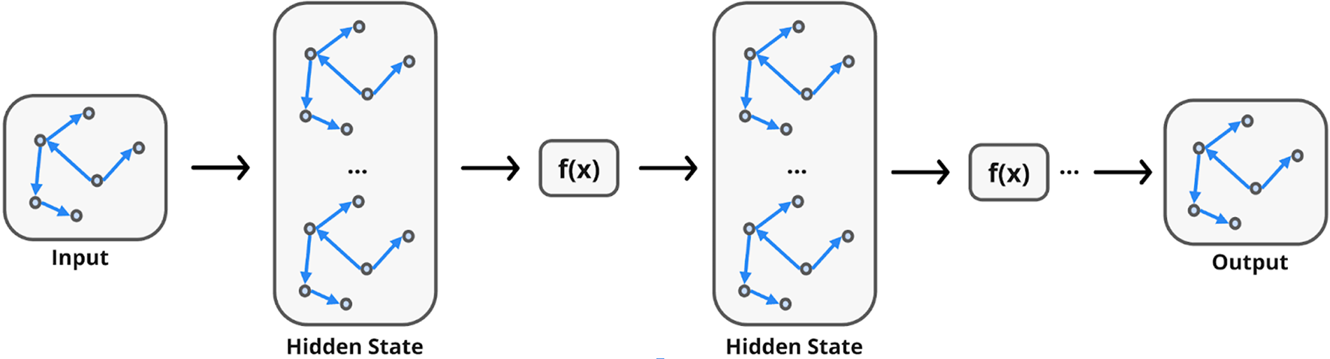
Figure 1: GNN networks

The financial domain is inherently relational and dynamic, making it well-suited for the application of Graph Neural Networks (GNNs). GNNs are increasingly used in tasks such as transaction network analysis, user-product interaction modeling, and stock relationship inference. They have demonstrated strong performance in applications including fraud detection and stock price prediction by effectively modeling the complex and evolving interdependencies characteristic of financial systems. However, the adoption of GNNs in FinTech also presents unique challenges. Financial data is often represented as time series or unstructured text, necessitating advanced preprocessing techniques to preserve temporal and semantic information. Additionally, the heterogeneous and dynamic nature of financial entities and interactions complicates graph construction and requires tailored GNN architectures capable of capturing both structural and contextual nuances for optimal performance.

Feature selection [5,6] is essential to mitigate the challenges posed by the high dimensionality and noise inherent in financial datasets. By isolating the most informative features, it reduces the complexity of the data, improves the generalization of the model, and enhances the overall performance of GNN-based systems. Although much of the existing research on GNNs emphasizes architectural innovations and algorithmic improvements, and many FinTech surveys concentrate on broader machine learning applications, the intersection of GNNs and feature selection remains underexplored. To date, few studies have systematically examined how feature selection can be effectively integrated with GNNs to address the unique demands of financial anomaly detection.

This paper fills that gap by providing an in-depth review of GNN applications in the financial sector, with a focus on anomaly detection. The report is structured as follows:

•   Section 2: Understanding anomalies in FinTech

•   Section 3: Understanding GNN networks

•   Section 4: Graph-based anomaly detection in FinTech

•   Section 5: Feature selection in FinTech

•   Section 6: Improving anomaly detection via feature selection and GNN integration

•   Section 7: Case studies and real-world applications

•   Section 8 and 9: Discussion and conclusions

This survey aims to serve as both a foundational reference and a practical guide for researchers and practitioners who wish to understand, implement, or innovate with GNNs in the context of financial anomaly detection, offering insights into the state-of-the-art methodologies and future research directions in this evolving field.

2  Understanding Anomalies in FinTech

In the realm of financial technology (FinTech), an anomaly [7–9] refers to any data point, transaction, or behavioral pattern that significantly deviates from the expected norms within a financial dataset. These deviations can signal a variety of critical events, including fraudulent transactions, attempts at market manipulation [10–12], system misuse, or even emerging trends in user behavior that may reveal new business opportunities. Detecting such anomalies is essential not only for preventing financial loss and ensuring regulatory compliance, but also for enhancing risk management and customer experience. Anomalies in FinTech are typically categorized into three major types:

1.    Global Outliers (Point Anomalies): These are individual data points that are vastly different from the rest of the dataset. For example, a single, unusually large transaction on a personal account could be a global outlier, possibly indicating fraudulent behavior or an operational error.

2.    Contextual Outliers (Conditional Anomalies): These occur when a data point is anomalous within a specific context, even if it might appear normal globally. For example, a $1000 transaction might be expected during the holiday season, but would be suspicious during a period of typically low spending or when made from a location the user has never visited.

3.    Collective Outliers: These involve a group of data points that, collectively, are anomalous in relation to the rest of the dataset. Individually, these points may not stand out, but taken together, they can indicate coordinated malicious activities such as a series of small unauthorized withdrawals, often a hallmark of fraud rings or account takeovers.

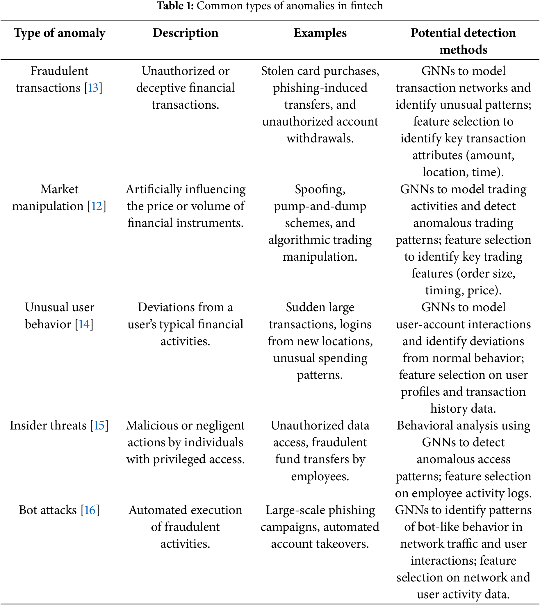
The FinTech landscape [11,12] is highly dynamic and data-rich, making it susceptible to a wide variety of anomalies. As illustrated in Table 1, each type presents distinct challenges and typically requires domain-specific detection techniques.

•   Fraudulent Transactions [13]: This is the most prominent and well-known category of anomalies. It includes:

–   Credit card fraud such as unauthorized transactions using stolen card data.

–   Chargeback fraud, when consumers dispute legitimate purchases to get refunds.

–   Loan fraud involves falsified documentation or synthetic identities.

–   Money laundering, where complex transaction sequences are used to obscure the origin of illicit funds.

–   Account Takeover (ATO), where hackers gain unauthorized access to a user’s financial account and conduct transactions under their name.

–   Phishing and identity theft involve the theft of sensitive data through deceptive tactics and used for financial gain.

•   Market Manipulation [12]: These anomalies affect financial markets and trading platforms, often with wide-reaching implications. Examples include:

–   Spoofing: Putting fake orders to mislead the market about demand or supply.

–   Pump-and-dump schemes: Artificially inflating the price of an asset by misleading information and then selling at the peak.

–   Algorithmic manipulation: Using algorithmic trading systems to create artificial volatility or exploit latency differences.

–   The emergence of Artificial Intelligence-generated (AI-generated) misinformation and social media manipulation has further amplified the risk of coordinated market anomalies.

•   Unusual User Behavior [14]: Behavioral anomalies are often early indicators of fraud or security breaches. These can include:

–   Uncharacteristic changes in spending habits.

–   Logins from unfamiliar IP addresses or geolocations.

–   Access accounts using new or suspicious devices.

–   Unusual transaction timing (for example, frequent midnight activity). Behavioral analytics powered by machine learning can detect these patterns in real time.

•   Insider Threats [15]: These are anomalies that arise from employees, contractors, or partners with privileged access. Insider threats may involve:

–   Intentional misuse, such as unauthorized access to confidential information or system tampering.

–   Accidental breaches, such as sending sensitive files to external recipients or misconfiguring security settings. Detecting insider threats requires analyzing both user behavior and access patterns across systems.

•   Bot Attacks and Automated Fraud [16]: Increasingly, attackers are using bots to automate a wide array of fraudulent actions. Examples include:

–   Credential stuffing, where bots attempt to log in using stolen username-password pairs.

–   Fake account creation, used to manipulate referral programs or conduct synthetic fraud.

–   Automated phishing campaigns and vulnerability scan. These attacks often leave behind distinctive patterns of access, transaction velocity, or IP address reuse.

Given the high stakes in financial systems, anomaly detection must go beyond simple rule-based filters. Modern detection systems must incorporate advanced techniques such as machine learning, graph analysis, and behavioral modeling to adapt to evolving threats. The complexity of FinTech data, often involving high-dimensional time series, user interactions, and transaction graphs, demands solutions that can scale, learn contextual signals, and identify both subtle and overt deviations.

Furthermore, integrating real-time detection capabilities is crucial, particularly for transaction monitoring and fraud prevention. Pairing AI-based models with human-in-the-loop oversight allows organizations to balance speed and accuracy, especially in ambiguous or high-impact cases.

In conclusion, anomaly detection in FinTech is a multifaceted challenge that spans domains from cybersecurity to behavioral science and financial engineering. A robust detection framework must be dynamic, interpretable and capable of integrating various data types to protect users and maintain trust in digital financial ecosystems.

3  Understanding GNN Networks

3.1 What Are Graph Neural Networks?

In computer science, a graph [3,4], as illustrated in Fig. 2, is a foundational data structure designed to model relationships between entities. It comprises nodes (also called vertices), which represent individual entities, and edges (also referred to as links or connections), which denote the relationships or interactions between these entities. Graphs are highly versatile and widely adopted in various domains to represent real-world systems such as social networks, biological systems, transportation networks, and the semantic web. Their flexible nature enables the modeling of complex interdependencies that cannot be easily captured by traditional data formats such as images or sequences.

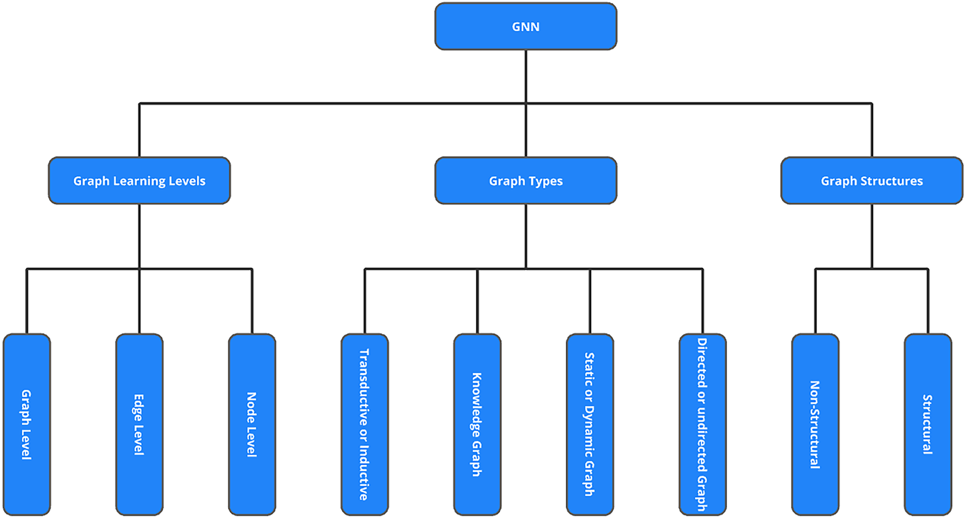
Figure 2: GNN taxanomy

The structure of graphs in Graph Neural Networks (GNNs) can be broadly divided into structural and non-structural scenarios. In structural settings, the graph topology is explicitly defined and derived from real-world relationships, as seen in applications such as molecular chemistry [17] (atoms as nodes and bonds as edges), physical systems, or knowledge graphs. In contrast, non-structural scenarios require the graph to be constructed from raw data, such as building a fully connected “word graph” from textual data or constructing a scene graph from an image. These distinctions affect how the graph is processed and what learning strategies are most effective.

Graphs also vary in type, each offering distinct properties. Directed graphs contain edges with a defined direction, indicating a one-way relationship from one node to another, while undirected graphs feature bidirectional edges, reflecting mutual relationships. Furthermore, graphs may be static, maintaining a fixed structure, or dynamic, where the graph evolves over time through the addition or removal of nodes and edges; social networks like Twitter are prime examples. Another important classification is between homogeneous and heterogeneous graphs. Homogeneous graphs consist of only one type of node and one type of edge, such as a traditional social network. In contrast, heterogeneous graphs [18] involve multiple types of nodes and edges, common in knowledge-based systems where entities such as people, organizations, and locations are interconnected through various types of relationships.

A notable example of a heterogeneous graph is the Knowledge Graph, which is typically expressed as triples in the form of (head, relation, tail) or (subject, relation, object). These graphs capture structured semantic relationships between real-world entities and are widely used in applications such as search engines, question answering, and intelligent recommendation systems [19].

In terms of learning paradigms, Graph Neural Networks (GNNs) are capable of operating in both transductive and inductive settings. In a transductive setting, the model is trained on a specific graph and tasked with inferring the labels of nodes within that same graph, which is effective when the entire graph structure is fully available during training. By contrast, inductive learning equips the model with the ability to generalize to unseen nodes or even entirely new graphs, making it particularly valuable for dynamic or evolving environments where graphs are continuously updated or expanded. Building upon these paradigms, recent research [4] has introduced Federated Graph Neural Networks (Federated GNNs), which integrate the principles of Federated Learning (FL) into GNN training. In this framework, clients such as banks, hospitals, or mobile devices collaboratively train a global GNN model while keeping their sensitive graph data local. Only model updates are shared, thereby preserving privacy and reducing regulatory concerns. This paradigm is highly relevant for sensitive application domains including finance, healthcare, cybersecurity, and recommendation systems, where safeguarding data privacy and ensuring compliance are essential.

GNNs are capable of handling a variety of learning tasks, which can be grouped into node-level, edge-level, and graph-level categories. At the node level, tasks involve predicting properties of individual nodes, for example, identifying whether a person in a social network is likely to be a smoker based on their connections. Edge-level tasks focus on relationships between nodes, such as predicting the likelihood of a new friendship in a social network or recommending the next video a user might watch on Netflix. Finally, graph-level tasks aim to infer properties of the entire graph, such as determining whether a molecular structure [17] has drug-like characteristics, a common task in computational chemistry.

Unlike regular data structures such as images (which follow a grid-like pattern) or text (which is sequential), graph data is inherently irregular and non-Euclidean. The nodes can have varying numbers of neighbors and the connections can form arbitrary patterns, making it challenging to apply conventional machine learning models. To address this, Graph Neural Networks have emerged as a powerful class of models specifically designed for graph-structured data. These networks operate via iterative message-passing mechanisms, where each node aggregates and transforms information from its neighbors to refine its representation.

Following a “graph-in, graph-out” paradigm, GNNs take an input graph where features can be embedded at the node, edge, or even graph level. As the data propagates through multiple neural layers, these embeddings are updated, capturing both local and global structural information. This enables the network to generate meaningful high-level representations while preserving the relational integrity of the original graph.

Due to their adaptability and expressiveness, GNNs have found applications across a wide array of domains, including recommendation systems, fraud detection, traffic forecasting, drug discovery, and knowledge-based inference. Their ability to learn from rich, interconnected data makes them an indispensable tool in modern AI research and real-world deployments.

3.2 GNN and How They Process Graph Data

Graph Neural Networks (GNNs) [1–4] operate fundamentally through the message passing paradigm (illustrated in Fig. 3), where nodes iteratively refine their internal representations by exchanging information with their neighbors. Through multiple layers of message passing, GNNs are able to capture both local structures (immediate neighbor patterns) and global dependencies (long-range interactions) within the graph.

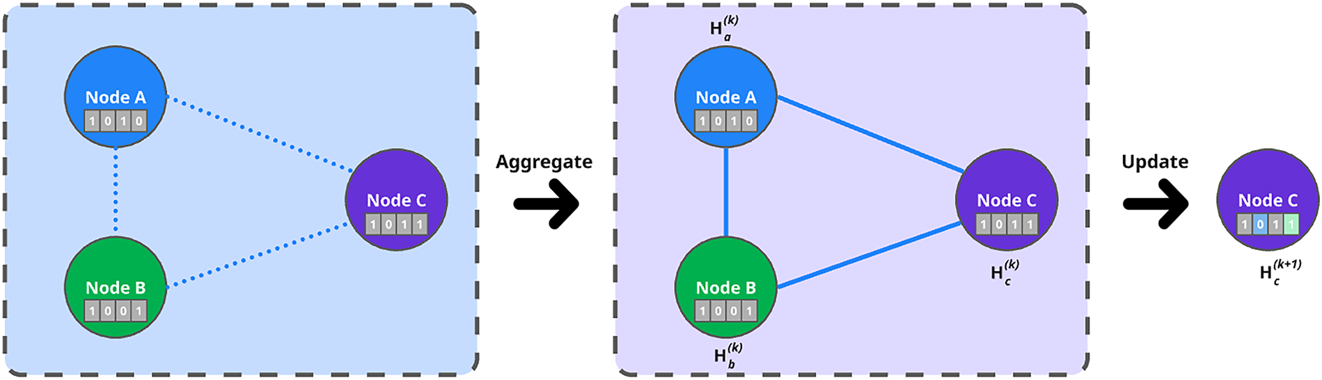
Figure 3: Message-passing paradigm

At each layer of a GNN, two primary computational steps are performed:

1. Message Passing (Aggregation): For each node, messages are received from neighboring nodes, consisting of either raw feature vectors or transformed embeddings. To guarantee consistency under any ordering of neighbors, the aggregation functions must exhibit permutation invariance. The standard operators used for this purpose include summation, mean, and maximum. This process is formally represented in Formula (1):

mv(k)=AGGREGATE(k)({hu(k):u∈𝒩(v)})(1)

where mv(k) denotes the aggregated message in layer k, hu(k) is the embedding of neighbor u, and 𝒩(v) denotes the set of neighbors of node v.

2. Node Update: After aggregation, each node refines its representation by integrating the incoming message with its existing embedding, as shown in Formula (2):

hv(k+1)=UPDATE(k)(hv(k),mv(k))(2)

where UPDATE(k) may be a neural network (e.g., an MLP) or a simple function such as addition.

Through successive layers of aggregation and update, nodes progressively accumulate information from larger neighborhoods, enabling the model to learn complex patterns across the graph.

Several architectural innovations have been proposed to address the challenges of learning on graphs:

1. Graph Convolutional Networks (GCNs) [20]: Extend the idea of convolution from grid-structured data (images) to graph-structured data. GCNs perform normalized weighted sums of neighbor features, leading to the update rule, as illustrated in Formula (3):

H(k+1)=D−12AD−12H(k)W(k)(3)

where A is the adjacency matrix with added self-loops, D is the corresponding degree matrix, H(k) is the embedding matrix of nodes in the layer k, and W(k) are learnable weights.

2. Graph Attention Networks (GATs) [21,22]: Introduce attention mechanisms to graph learning, allowing nodes to assign different importance scores to different neighbors, as illustrated in Formula (4):

αij=exp⁡(LeakyReLU(a→⊤[Whi||Whj]))∑k∈𝒩(i)exp⁡(LeakyReLU(a→⊤[Whi||Whk]))(4)

where αij is the attention coefficient between node i and node j, || denotes concatenation, and a→ and W are learnable parameters.

3. GraphSAGE [23]: Focuses on scalability for large graphs by introducing neighborhood sampling and fixed size aggregation (e.g., via mean or LSTM-based pooling) rather than aggregating information from all neighbors, as illustrated in Formula (5):

hv(k+1)=σ(W(k)⋅AGGREGATE(k)({hv(k)}∪{hu(k):u∈Sample(𝒩(v))}))(5)

where hu(k) is the embedding of node u in layer k, σ(⋅) is an activation function (e.g., ReLU), 𝒩(v) denotes the neighbors of v, and AGGREGATE is a learnable or predefined function.

Training of GNNs typically involves minimizing a task-specific loss function, such as cross entropy for classification or margin-based losses for link prediction. During training, GNNs learn the parameters of aggregation and update functions to optimize performance on labeled data.

A central outcome of GNN architectures [24] is the embedding of graph nodes in a low-dimensional continuous vector space, where proximity reflects structural similarity, role similarity, or feature similarity. These learned embeddings can then be used for a variety of downstream machine learning tasks, including:

•   Node classification (e.g., fraud detection)

•   Link prediction (e.g., transaction recommendation)

•   Graph classification (e.g., predicting systemic financial risk)

Because GNNs naturally preserve both local and global graph information in these embeddings, they are powerful tools for analyzing complex, relational data structures in domains like social networks, biological systems, and financial transaction graphs.

3.3 Applications of GNNs

Graph neural networks (GNNs) [1–3] have demonstrated remarkable versatility and effectiveness in a wide range of domains, primarily due to their ability to model complex relational structures inherent in graph-structured data. In the financial technology (FinTech) sector, GNNs [25] are increasingly applied to anomaly detection, particularly to identify fraudulent activities and patterns of irregular transactions. By capturing intricate relationships among accounts, transactions, and financial entities, GNNs enable more precise and context-aware detection systems.

In addition, in social network analysis, GNNs are used to uncover community structures, identify influential users, and predict user behavior utilizing patterns in user interactions and network topology. Recommender systems benefit from GNNs [19,26] by modeling user-item interaction graphs. This facilitates more personalized and accurate recommendations by incorporating both direct and indirect relationships within the network.

Furthermore, in bioinformatics and drug discovery, GNNs [27,28] model molecules as graphs-where atoms serve as nodes and chemical bonds as edges-allowing accurate prediction of molecular properties, interactions and potential drug efficacy. In healthcare, GNNs [29,30] are used to detect medical misinformation and support clinical decision-making by integrating structured medical knowledge into the learning process, thus improving the contextual reasoning capabilities of the model.

The intelligent transportation sector also uses GNNs [31,32] for traffic forecasting, where intersections and roads are represented as nodes and edges. This allows models to learn spatial-temporal patterns and improve predictions of congestion and flow dynamics.

In industrial manufacturing, GNNs [33] are deployed for fault diagnosis by modeling sensor relationships, component interactions, and process flows, outperforming traditional methods that often struggle with relational complexity.

Finally, in computer vision, GNNs are used to represent images and video scenes as graphs, capturing spatial relationships between objects or regions. This graph-based representation supports tasks such as object detection, scene understanding, and visual reasoning in a more structured and context-aware manner.

The practical success of GNNs [28] is highlighted by their adoption in production systems by major technology companies such as Uber, Google, Alibaba, Pinterest and Twitter. These organizations leverage GNNs for tasks like fraud detection, content recommendation, user engagement modeling, and knowledge graph reasoning, often reporting substantial performance gains over traditional deep learning models. Core graph-based tasks enabled by GNNs include:

•   Node Classification: Assigning labels to individual nodes (e.g., user type, product category).

•   Graph Classification: Adding labels to entire graphs (e.g., molecule toxicity, user intent).

•   Link Prediction: Inferring missing or future connections between nodes (e.g., friend suggestions, molecular binding).

•   Anomaly Detection: Identifying unusual patterns, outliers, or suspicious entities within a graph.

As research continues and tooling improves, GNNs are expected to play an even greater role in solving problems across scientific, industrial, and commercial domains, wherever relationships between entities matter.

4  Graph-Based Anomaly Detection in FinTech

4.1 Types of Abnormalities in Graph Data

Anomaly detection [34,35], also known as outlier detection, is a key task in data mining that focuses on identifying rare or atypical data points that significantly diverge from expected norms. When extended to graph-structured data, the challenge deepens, as anomalies may manifest at various levels, including nodes, edges, subgraphs, or entire graphs, through unusual properties or structural roles that stand out from the broader network. This complexity is amplified in dynamic or adversarial environments, where the definition of “normal” evolves over time, requiring adaptable and context-sensitive detection strategies. Unlike noise removal, which targets irrelevant or corrupted data, anomaly detection aims to surface meaningful deviations that often correspond to high-impact events such as fraud, cyber intrusions, or system breakdowns.

The practical value lies in the real-world relevance of these outliers, especially in domains such as e-Commerce, finance, or network security, where early identification of suspicious behavior can safeguard operations and build user trust. Graph Neural Networks (GNNs) are particularly well suited for this task, as their message-passing mechanisms allow them to learn expressive, context-aware representations by integrating both node attributes and the underlying relational structure. Depending on the type of anomaly, GNN-based models can be tailored accordingly: node-level models detect suspicious user profiles, edge-level architectures identify unexpected or inconsistent connections, subgraph models reveal collusion clusters or fraud rings, and graph-level encoders capture large-scale behavioral shifts across systems or time.

As illustrated in Table 2, anomalies in graph data can be classified according to the structural level at which they emerge:

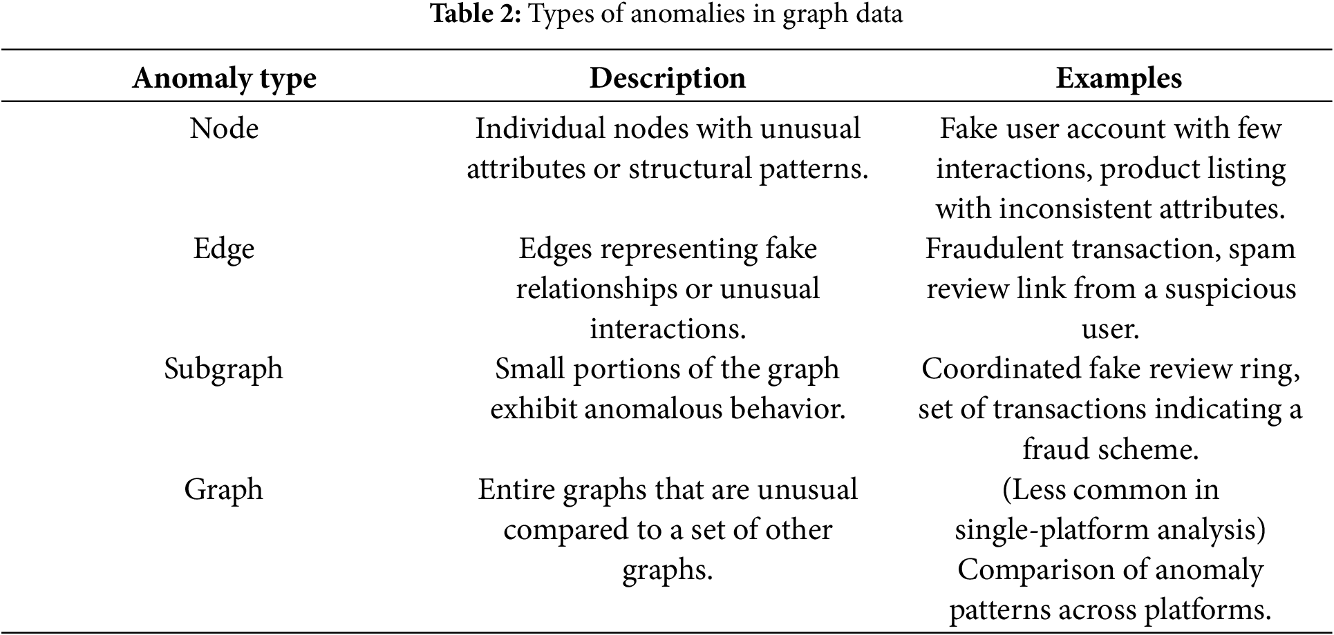
1. Node Anomalies [36]: These involve individual nodes whose features or structural positions deviate from expectations. A node might be anomalous due to the following:

•   Irregular feature values (e.g., demographic or behavioral attributes).

•   Unusual degree (too many or too few connections).

•   Isolation from communities or clusters.

Example: A fake customer account that has no purchase history but suddenly posts numerous reviews, or a product entry with inconsistent category labels and prices.

2. Edge Anomalies [36]: Edge anomalies represent irregular relationships between nodes. They might involve:

•   Unexpected links between nodes that normally do not interact.

•   Abnormal interaction weights (too frequent or rare).

•   Cross-community edges that don’t fit existing network patterns.

Example: A suspicious purchase transaction between two unrelated accounts or a review submitted by a user who has never interacted with similar products.

3. Subgraph Anomalies [36]: These refer to collections of nodes and edges that, as a group, behave in a way that is inconsistent with the broader network. Subgraph anomalies may feature the following:

•   Dense or repetitive interaction patterns.

•   Rare motifs or structural configurations.

•   Isolated cliques with coordinated behavior.

Example: A group of users who post similar reviews on the same products in a short period of time, which could indicate a fraudulent review campaign.

4. Graph-Level Anomalies [36,37]: When analyzing a set of graphs, such as between different periods or systems, entire graphs can be considered anomalous based on their global structure, node distributions, or interaction patterns. Example: An e-commerce site graph from a particular week that shows a sudden shift in user behavior or transaction patterns, possibly due to a bot attack or external event. This type of anomaly is particularly relevant in trend analysis or cross-platform comparisons.

4.2 Advantages of GNNs for Anomaly Detection

The FinTech and e-Commerce domains [38–42] present exceptionally rich environments for anomaly detection, driven by their complex, high-volume, and multi-relational nature. Millions of users, products, reviews, and transactions interact in real time, creating dynamic graphs saturated with legitimate and malicious activities. This complexity generates diverse types of anomalies, each offering unique challenges and opportunities where Graph Neural Networks (GNNs) can demonstrate their full potential.

Fraud in these environments takes many forms, including high-value transactions from newly created accounts, repeated large purchases from the same IP address, suspicious payment methods, or abrupt changes in billing information. Such activities often leave subtle but structured patterns within transaction graphs, manifesting as tightly connected fraudulent clusters or abnormal transaction flows. GNNs, adept at modeling relational irregularities, can learn hidden transaction patterns between users, payment tools, and merchants, making them particularly effective in revealing fraud.

Customer reviews are central to e-Commerce trust, yet are frequently targeted for manipulation. Spam reviews, designed to artificially inflate or deflate product ratings, often originate from fake or compromised accounts that display atypical behaviors, such as extremely short review intervals, uniform sentiments [43] across unrelated products, or unusual product reviewer-linking patterns. By constructing reviewer-product graphs, where nodes represent users and products and edges represent review interactions, GNNs can learn to detect anomalies at both the individual and community levels, identifying suspicious accounts and clustered abnormal behaviors.

Beyond financial fraud, threats such as account takeovers and bot activities are major concerns. Indicators such as abnormal browsing behaviors, erratic clickstreams, irregular cart additions, or sudden purchasing spikes suggest compromised or automated accounts. Building temporal graphs [44], such as user-product interaction sequences or session graphs, allows GNNs to capture both static anomalies and temporal deviations. This capability enables early detection of emerging fraudulent activities or coordinated bot attacks that traditional feature-based methods often miss.

Given the multifaceted and evolving nature of anomalies in FinTech and e-commerce, GNNs provide a uniquely powerful and adaptable framework. They enable joint learning over both feature information (e.g., user demographics, product metadata) and relational structures (e.g., transaction graphs, review networks) via message passing. GNNs naturally aggregate multi-hop neighborhood information, a critical feature for detecting complex, coordinated frauds, such as colluding account rings. Moreover, the same GNN model can flexibly target node-level (e.g., user fraud detection), edge-level (e.g., suspicious transaction detection) or graph-level (e.g., anomalous session behavior) anomaly tasks.

A fundamental step for effective GNN deployment is careful graph construction [1]. This phase defines how well relational and contextual signals are captured. The nodes typically represent heterogeneous entities, including users, products, transactions, reviews, and merchants, each augmented with rich feature vectors. For example, user nodes might encode account age, historical purchasing behavior, log-in devices, and preferred payment methods; product nodes can include attributes such as category, price, brand reliability, and cumulative rating trends; transactions can be modeled as edges or standalone nodes enriched with amount, time, location, and device data; while reviews can integrate textual embeddings, sentiment scores, and reviewer activity features. Merchants may also be characterized by factors such as return rates, dispute histories, and average order values.

Edges capture crucial relational dynamics, including user-product purchases, user-review authorships, and merchant-user transactions. These edges can be weighted by frequency, transaction value, or recency, adding critical temporal and contextual information. User-user connections based on shared IPs, behavioral similarities, or merchant-user edges reflecting buyer-seller relationships further enrich the graph, creating a comprehensive relational blueprint for anomaly detection.

The inherently heterogeneous structure of FinTech and e-Commerce datasets, spanning diverse nodes and edges, makes them ideal for heterogeneous graph modeling. Unlike homogeneous graphs that treat all entities uniformly, heterogeneous graphs allow GNNs to differentiate between node types and relation-specific dynamics, learning richer and more expressive representations. Specialized architectures such as Relational Graph Convolutional Networks (R-GCN) [45] and Heterogeneous Graph Attention Networks (HAN) [46] are particularly effective in leveraging these structures, significantly enhancing anomaly detection performance.

In conclusion, the FinTech and e-commerce landscapes, with their complexity, velocity, and high financial stakes, offer an ideal proving ground for GNN-based anomaly detection frameworks. By carefully constructing heterogeneous graphs and leveraging GNNs’ powerful relational reasoning abilities, it becomes possible to uncover sophisticated fraud, spam, and behavioral anomalies that traditional machine learning approaches would often overlook.

4.3 GNN-Based Anomaly Detection Methods

Graph Neural Networks (GNNs) [38–42] have demonstrated remarkable adaptability for various anomaly detection tasks in graph-structured data. Their effectiveness largely depends on how the anomaly detection problem is framed and the specific GNN architecture employed.

At the node level, GNNs learn embeddings hv that encode the structural and attribute-based context of a node. These embeddings are then used to classify nodes as normal or anomalous. Formally, the embedding update at layer k can be expressed as Formula (6):

hvk+1=(Wk⋅AGGREGATEk({huk,u∈N(v)}))(6)

where Wk are trainable weights, N(v) denotes the neighbors of node v, and AGGREGATE is a learnable or predefined function.

In graph-level classification, GNNs compute a graph embedding by pooling node representations, as illustrated in Formula (7):

hG=READOUT({hv,v∈G})(7)

where READOUT can be simple (mean, sum) or complex (attention-based). The pooled embedding hG is then used to determine whether the entire graph is anomalous.

For link prediction, GNNs estimate the likelihood of an edge between two nodes u and v based on their embeddings, as shown in Formula (8):

Pr(euv=1)=(huhv)(8)

where euv indicates the existence of an edge.

In subgraph anomaly detection, GNNs often rely on Graph Autoencoders (GAEs). The GAE framework consists of an encoder f and a decoder g, trained to minimize reconstruction loss, as illustrated in Formula (9):

Lrecon=∑(u,v)∈E(euv−e^uv)2,where e^uv=g(f(hu),f(hv))(9)

Nodes, edges, or subgraphs with high reconstruction error are marked as anomalous.

Another emerging strategy is contrastive learning [4,38,39], in which GNNs are trained to differentiate between similar (positive) and dissimilar (negative) pairs. A typical contrastive loss is illustrated in Formula (10):

Lcontrastive=−log⁡exp⁡(sim(hu,hv)/τ)∑w∈𝒩exp⁡(sim(hu,hw)/τ)(10)

where sim(⋅,⋅) is a similarity measure (e.g., cosine similarity), τ is a temperature parameter, and 𝒩 denotes the set of neighbors of node u. In contrastive learning for GNNs, the contrastive loss plays a dual role by simultaneously pulling together embeddings of positive node or graph pairs, such as two augmented views of the same instance or structurally/semantically related neighbors, while pushing apart negative pairs that are unrelated or come from different contexts. By maximizing the similarity of positives, the model preserves local consistency, structural information, and semantic alignment within the graph, ensuring that representations of related entities remain close in the embedding space. At the same time, by minimizing the similarity to negatives, the loss enhances the discriminability of the learned embeddings, preventing collapse into trivial solutions and encouraging a clear separation between distinct graph components. This balance enables the GNN to capture both fine-grained relational dependencies and global contrastive distinctions, ultimately leading to more robust, generalizable graph representations for downstream tasks such as classification, clustering, and link prediction.

The strength of GNNs in anomaly detection lies in their ability to jointly exploit node features and graph structure via message passing. In particular, homophily, the tendency of connected nodes to exhibit similar properties, can be used to detect nodes that deviate from the expected local patterns.

The choice of graph construction significantly influences the performance of the anomaly detection pipeline. A graph tailored for fraud detection might emphasize transaction and user-product relationships, whereas one for spam detection might focus on review and reviewer-product links.

As illustrated in Table 3, GNN-based approaches to anomaly detection can be broadly categorized by their methodological foundations:

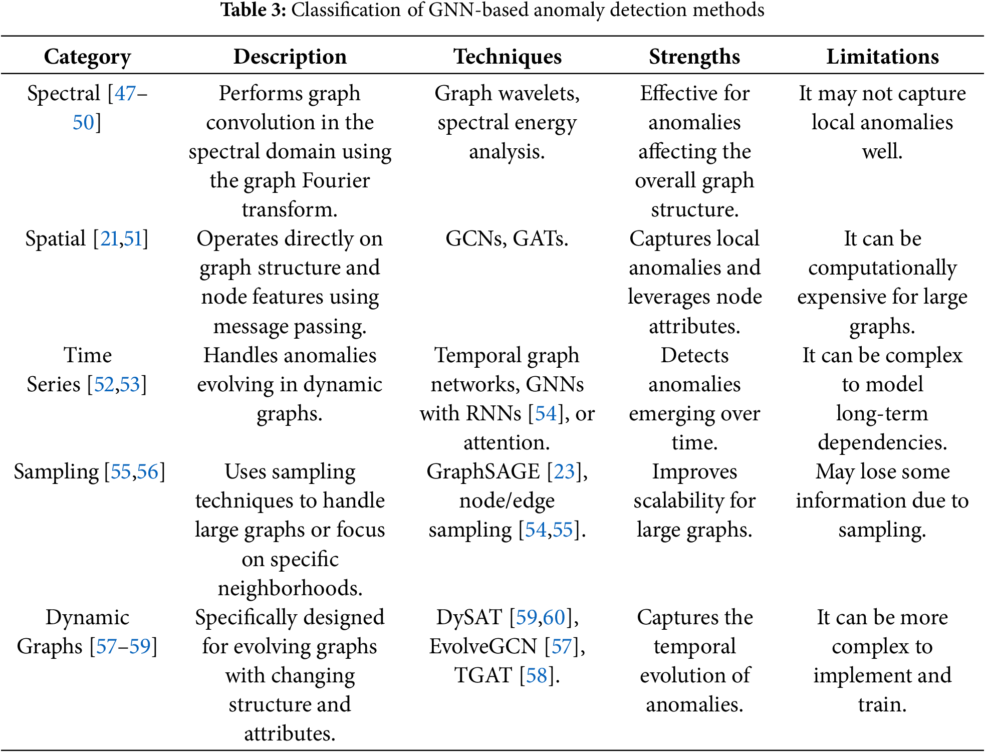
1. Spectral Methods [47–50]: These operate in the spectral domain of the graph, utilizing the eigenvalues and eigenvectors of the Laplacian graph L = D − A, where D is the degree matrix and A is the adjacency matrix. Anomalies are identified through disturbances in the spectral properties. A common spectral convolution operation is illustrated in Formula (11):

g(L)x=Ug(Λ)Ux(11)

where U is the matrix of eigenvectors, Λ is the diagonal matrix of eigenvalues, and g(⋅) is a spectral filter function that can be learned.

2. Spatial Methods [21,51]: These rely on message passing directly in the graph domain, aggregating information from neighbors. A standard spatial aggregation for node v in layer k is as illustrated in Formula (12):

hvk+1=σ(∑u∈N(v)1cvuWkhuk)(12)

where cvu is a normalization constant (e.g., degree-based), Wk are trainable weights, and σ is a non-linear activation function.

3. Time-Series Approaches [52,53]: Given that FinTech data often evolves over time, dynamic graphs Gt=(Vt,Et) are modeled. GNNs are extended with temporal models like RNNs or attention mechanisms. A basic temporal embedding update using an RNN can be presented in Formula (13):

hvt=RNN(hvt−1,GNN(Gt−1,hvt−1))(13)

where the RNN [54] (e.g., LSTM) captures sequential dependencies across time steps. These methods detect anomalies that emerge from changes in behavior patterns or network dynamics over time.

4. Sampling-Based Techniques [55,56]: Large-scale graphs require computational efficiency. Methods like GraphSAGE [23] aggregate information from a sampled subset of neighbors. The sampled aggregation at node v is as illustrated in Formula (14):

hvk+1=(Wk⋅AGGREGATEk({huk,u∈Sample(N(v))}))(14)

where Sample(N(v)) denotes a random or importance-based sample of neighbors. This improves scalability, but may lose critical information for detecting rare anomalies.

5. Dynamic Graph Techniques [57–59]: These models explicitly account for evolving graph structures and node attributes. For example, EvolveGCN dynamically updates GNN weights based on graph evolution, as illustrated in Formula (15):

Wtk=RNN(Wt−1k,GraphContextt)(15)

where Wtk are the layer weights at time t and GraphContextt encodes temporal features from the current graph snapshot.

5  Feature Selection in FinTech

Feature selection [5,6] is a critical component of the machine learning pipeline, particularly in domains characterized by high-dimensional data, such as the financial technology (FinTech) sector. It involves the systematic identification and retention of the most informative and relevant features, also known as variables or predictors, while eliminating those that are redundant, irrelevant, or noisy. This process not only reduces the dimensionality but also improves the performance, generalization, and computational efficiency of the model.

High-dimensional financial data such as transaction records, user behavior metrics, and market indicators are often susceptible to the “curse of dimensionality” wherein an abundance of features can obscure meaningful patterns and degrade model accuracy. By focusing on a compact set of discriminative variables, feature selection facilitates more effective pattern learning, accelerates convergence during training, and enhances generalization to unseen data.

In addition to boosting predictive performance, feature selection also reduces computational overhead, which is particularly advantageous in real-time FinTech applications such as fraud detection, credit scoring, and risk assessment. Furthermore, by producing more concise and transparent models, feature selection enhances interpretability, an essential requirement in regulated financial environments where explainability is crucial for accountability and compliance.

Importantly, feature selection acts as a safeguard against overfitting, where a model memorizes noise in the training data rather than learning generalizable patterns. In the context of anomaly detection in FinTech, where identifying rare but impactful events (e.g., fraudulent transactions or credit default risks) is mission critical, effective feature selection helps isolate the signals that truly matter. This ensures that the models remain robust even when faced with noisy, complex, or evolving financial environments.

5.1 Feature Selection Techniques

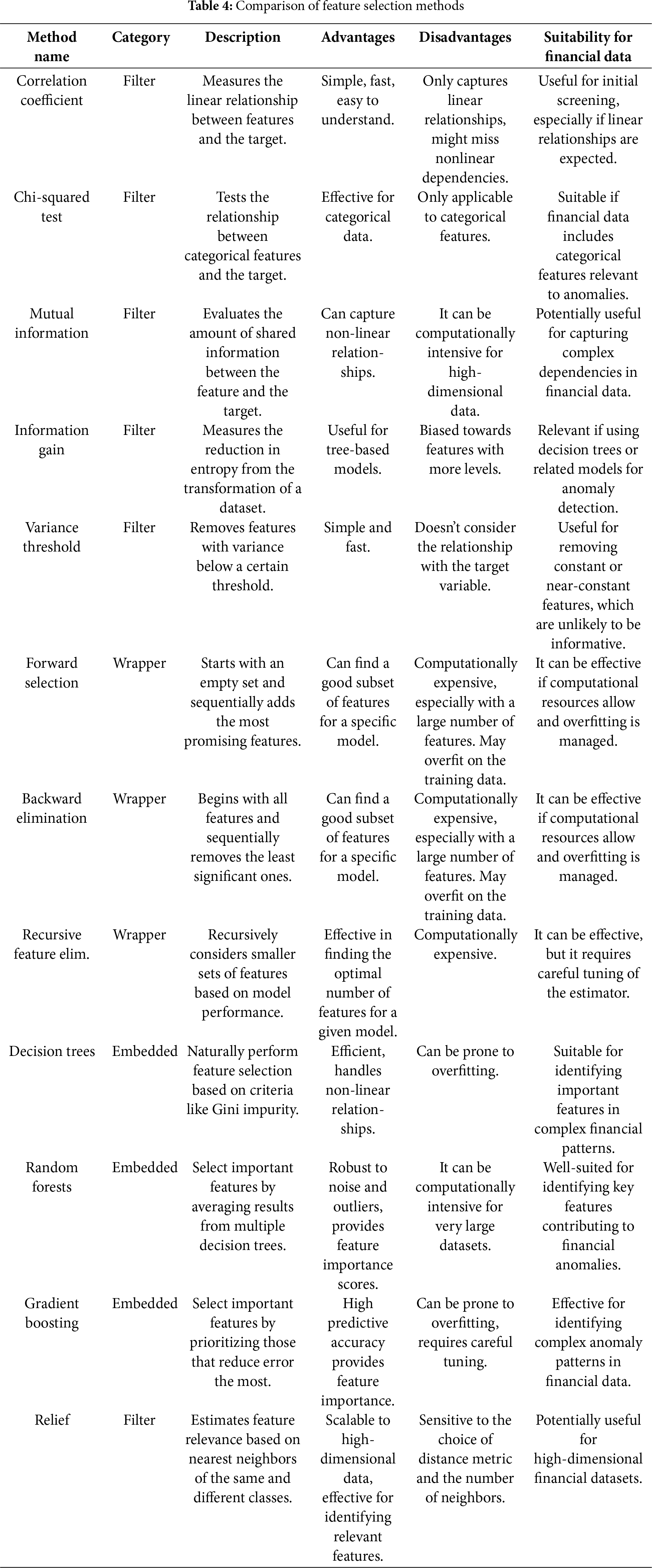
As illustrated in Table 4, feature selection techniques [61,62] are commonly categorized into three main classes: filter methods, wrapper methods, and embedded methods, each offering distinct advantages depending on the use case and computational constraints.

5.1.1 Filter Methods

Filter methods [61–63] constitute a foundational class of feature selection techniques that evaluate features independently of any specific machine learning model. As illustrated in Fig. 4, these methods are based on the statistical characteristics of individual characteristics and their direct relationship with the target variable, making them computationally efficient and highly scalable, particularly well suited for high-dimensional datasets common in FinTech applications.

Figure 4: Filter method

Various statistical metrics are commonly used in filter methods. The correlation coefficient assesses the strength and direction of a linear relationship between continuous features and the target variable. The Chi-Squared test evaluates the association between categorical variables and the target and is frequently used in classification tasks. Mutual information (or information gain) measures both linear and non-linear dependencies, capturing how much information one variable provides about another. Fisher’s score quantifies the discriminative power of a feature by comparing the variance between classes and between classes. Variance thresholding removes features with low variance, assuming that features with little variability are unlikely to be informative. Finally, the dispersion ratio helps identify features that exhibit a distinct separation between classes, making it valuable for feature selection in classification problems.

In general, filter methods offer a fast, model-agnostic approach to initial feature screening and are often employed as a preliminary step prior to the application of more computationally intensive wrapper or embedded techniques. Among these, the Pearson correlation coefficient is a widely used metric to evaluate the linear relationship between a continuous feature x and a target variable y. It is defined as illustrated in Formula (16):

r=∑i=1n(xi−x¯)(yi−y¯)∑i=1n(xi−x¯)2∑i=1n(yi−y¯)2→a.s.ρ=Cov(X,Y)σXσY(16)

where x¯ and y¯ are the mean values of x and y, respectively, and σX2=Var(X) and σY2=Var(Y). A high absolute value of r indicates a strong linear relationship, making the feature more relevant for prediction tasks. The sample Pearson correlation r converges almost surely to the true population correlation ρ by the law of large numbers. Moreover, it converges at a rate of 1/n and is asymptotically normal, which allows us to construct confidence intervals and perform hypothesis tests.

Filter methods offer several advantages: they are computationally efficient, model-independent, and highly scalable, making them particularly useful when working with large feature sets. However, a major limitation is that they treat features independently, ignoring possible interactions between them that could enhance model performance. As a result, while filter methods are excellent for initial feature selection, they are often best used in combination with other methods for more robust modeling.

5.1.2 Wrapper Methods

Wrapper methods [61,62,64] are a powerful class of feature selection techniques that differ significantly from filter and embedded methods. As shown in Fig. 5, these methods are model-specific and rely on iterative training and evaluation of machine learning algorithms using different subsets of characteristics. Unlike filter methods, which use statistical measures to rank features independently of the chosen model, wrapper methods integrate feature selection with the model training process itself, making them highly tailored to the specific algorithm used. While this results in higher computational complexity, it also tends to yield superior performance, particularly when the interaction between features is important for the model’s predictive power.

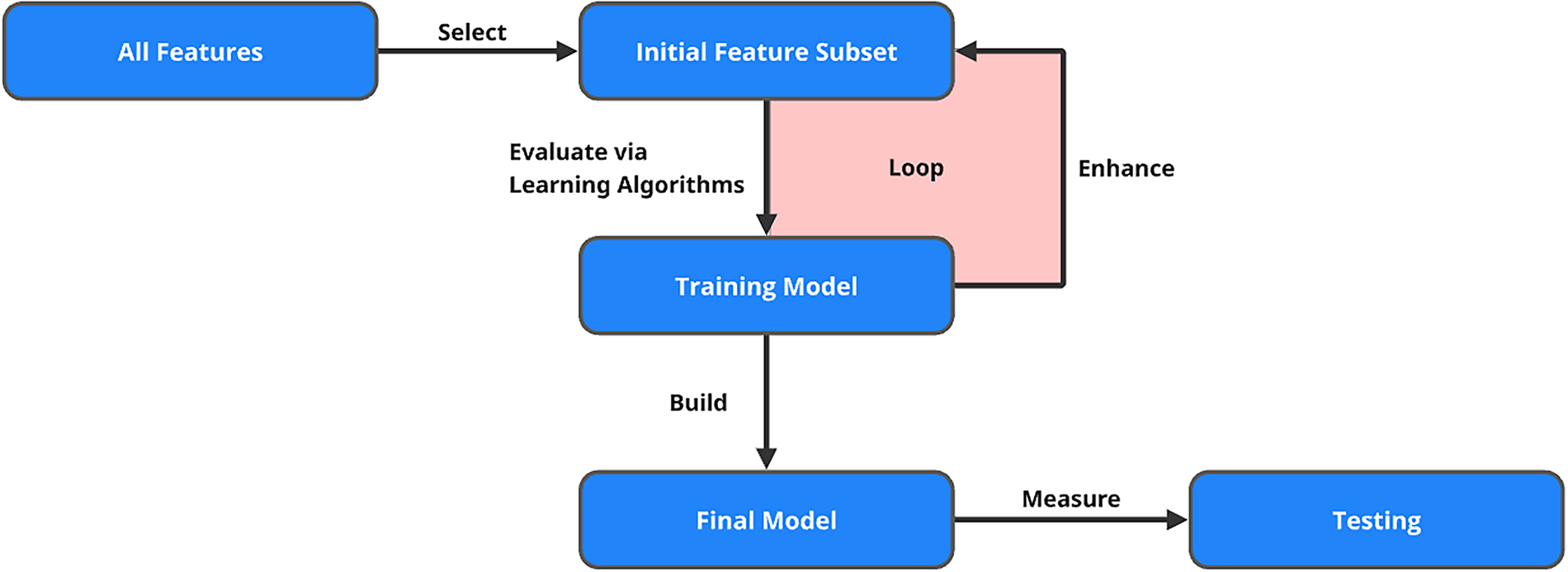
Figure 5: Wrapper method

The heart of the wrapper methods is the search for the optimal subset of features, denoted by S∗, which maximizes the performance of the model. The process involves repeatedly training a model on various subsets of features and evaluating its performance using a chosen evaluation metric, M. The subset of features S that leads to the highest metric value is selected as the best feature set. The mathematical formulation of this process can be expressed in Formula (17):

S∗=arg⁡maxS⊆{1,…,p}M(f(XS),y)(17)

where:

•   S is a subset of features.

•   f(XS) is the output of the model when trained on the feature subset XS.

•   M(f(XS),y) is the evaluation metric (e.g., accuracy, precision, recall) that measures how well the model predictions match the true labels y.

•   p is the total number of features.

•   S∗ represents the optimal subset of features that maximizes the evaluation metric.

Forward selection starts with no features in the model and iteratively adds features that improve the model’s performance. At each step, the feature that provides the highest increase in the evaluation metric is selected and added to the subset. This process continues until adding more features does not yield a significant improvement in performance:

1.   Begin with an empty feature set S.

2.   Train the model with each feature individually and add the feature that maximizes the performance.

3.   Repeat the process, adding one feature at a time, until further addition no longer improves the model.

In backward elimination, the process begins with all available features and removes the least significant ones iteratively. At each step, the feature that contributes the least to the model’s performance is removed, and the model is retrained. The process continues until removing features no longer results in a meaningful drop in performance:

1.   Start with the full set of features S = {1, 2, … , p}.

2.   Evaluate the model with all features and remove the least important feature based on the evaluation metric.

3.   Repeat the process, removing features one at a time, until only the most significant features remain.

Recursive Feature Elimination (RFE) is a more sophisticated technique that recursively removes features based on their importance, as determined by the model’s coefficients or feature importance scores. After each iteration, the least important feature is removed, and the model is retrained. RFE continues until the optimal subset of features is identified:

1.   Start with all features and train the model.

2.   Rank the features based on their importance scores (e.g., coefficients for linear models or feature importances for tree-based models).

3.   Remove the least important feature and retrain the model.

4.   Repeat the process until the desired number of features is selected.

The exhaustive search is the most computationally expensive method, in which all possible subsets of features are evaluated. This method guarantees finding the optimal feature subset, but it is only feasible for small datasets due to its combinatorial nature, as the number of subsets grows exponentially with the number of features:

1.   Evaluate the model with every possible combination of features.

2.   Select the feature subset that provides the best performance based on the evaluation metric.

Wrapper methods offer several advantages:

1.   Interactivity: Wrapper methods account for feature interactions, meaning they don’t just evaluate individual features in isolation. Instead, they assess how features work together in the context of the model. This leads to potentially better performance, especially for models that are highly sensitive to feature interactions, such as decision trees and neural networks.

2.   Customizability: Since wrapper methods directly incorporate the machine learning algorithm into the feature selection process, they can be tailored specifically to the model. This means that the feature selection process is optimized for the strengths and weaknesses of the chosen algorithm, leading to better results compared to more general methods.

3.   Optimality for the Model: Wrapper methods optimize feature selection with respect to the model performance metric. This leads to feature subsets that are well-suited for the specific algorithm, improving the model’s predictive power.

However, wrapper methods come with their own set of drawbacks:

1.   Computational Expense: Wrapper methods are computationally intensive because they require multiple iterations of training and evaluation with different subsets of features. As the number of features grows, the search space increases exponentially, making these methods impractical for very large datasets or when the feature set is large (e.g., thousands of features).

2.   Risk of Overfitting: Because wrapper methods are highly tailored to the training data, there is a risk of overfitting, particularly when the dataset is small. The model may select feature subsets that perform well on the training data but fail to generalize to unseen data. This can result in a model that is too complex or too tuned to the specific features of the training set.

3.   High Resource Consumption: Due to the iterative nature of training models with different subsets of features, wrapper methods require significant computational resources, especially when dealing with large datasets. This can be a limitation in real-world scenarios where computational power is constrained.

Wrapper methods are most effective in situations where:

•   Feature Interactions are Important: When the interaction between features significantly impacts the model’s performance, wrapper methods are a good choice as they evaluate these interactions.

•   Dataset Size is Manageable: If the dataset is not too large and computational resources are sufficient, wrapper methods can be highly effective.

•   Model-Specific Optimization is Needed: When working with a particular machine learning algorithm, wrapper methods can fine-tune the feature selection process for that model, leading to optimal performance.

Wrapper methods offer a robust and highly customizable approach to feature selection, often leading to superior model performance. However, they come with trade-offs in terms of computational cost and potential for overfitting. These methods should be used when the dataset size is manageable and when feature interactions are expected to have a significant impact on the model performance. For larger datasets, or when feature sets are extremely large, alternative methods like filter or embedded techniques might be more practical.

5.1.3 Embedded Methods

Embedded methods [61,62,65] perform feature selection as an integral part of the model training process, allowing the algorithm to automatically identify and retain the most relevant features while fitting the model. As shown in Fig. 6, these methods strike an effective balance between computational efficiency and predictive performance by combining the strengths of both filter and wrapper approaches.

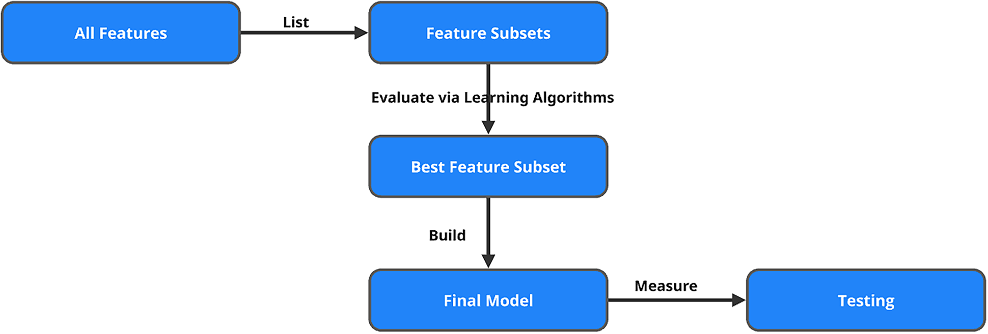
Figure 6: Embedded method

Unlike filter methods that evaluate features independently of the model or wrapper methods that iteratively evaluate subsets of features, embedded methods incorporate feature selection directly into the training algorithm. This integration not only reduces redundancy but also enhances the model’s ability to generalize by prioritizing informative variables and discarding irrelevant or redundant ones.

Many machine learning algorithms inherently support embedded feature selection. For example:

•   Decision Trees, Random Forests, and Gradient Boosting Machines (GBMs) naturally evaluate feature importance based on how well each feature improves decision splits or reduces loss. These models assign importance scores during training, allowing features to be automatically ranked and selected.

•   Regularization techniques like Lasso Regression (L1 regularization) and Elastic Net implicitly perform feature selection by penalizing the inclusion of less informative features. In these models, the feature coefficients are shrinkage during training, and some may be driven exactly to zero, effectively removing them from the model.

Lasso regression introduces an L1 penalty to the standard linear regression objective, encouraging sparsity in the model coefficients, as illustrated in Formula (18):

minβ12n∑i=1n(yi−∑j=1pxijβj)2+λ∑j=1p|βj|(18)

Here, λ is the regularization parameter that controls the strength of the penalty. As λ increases, more coefficients are driven to zero, effectively selecting only the most predictive features:

•   Lasso Regression (L1 Regularization): Promotes sparsity by penalizing the absolute size of coefficients.

•   Elastic Net: Combines both L1 and L2 penalties, balancing variable selection and coefficient stability.

•   Decision Trees and Ensembles (Random Forests, GBMs): Implicitly rank feature importance as part of the model’s structure.

Embedded methods offer a powerful model-aware approach to feature selection by integrating the selection process directly into model training, thereby balancing efficiency and performance. Their key strengths include efficiency, as feature selection occurs within the training phase without requiring a separate step; robustness, since the resulting models often generalize better and are less prone to overfitting; and interaction awareness, enabling the capture of complex feature interactions that filter methods may miss. However, embedded methods also come with limitations: the selected features are often highly dependent on the specific algorithm used, which may reduce generalizability across models, and their interpretability can be limited, especially in complex ensemble models, making it difficult to understand why certain features were chosen or discarded. Despite these challenges, embedded methods remain a scalable and effective solution, particularly well-suited for high-dimensional datasets where traditional methods may struggle.

5.2 High-Dimensional and Noisy Financial Data

Applying traditional feature selection techniques to financial datasets presents a range of intricate challenges, largely due to the high dimensionality, heterogeneity, and inherent noise of financial data. High dimensionality, where the number of features is large relative to the number of observations, invokes the curse of dimensionality, making the feature space increasingly sparse. This sparsity undermines distance metrics such as the Euclidean distance, as illustrated in Formula (19):

d(xi,xj)=∑k=1p(xik−xjk)2(19)

which lose discriminatory power as differences across features converge toward uniformity. Consequently, models struggle to discern meaningful patterns, increasing the likelihood of overfitting and diminishing the performance of standard feature selection methods. Further compounding the issue, financial data often contains noise, missing values, and inconsistencies due to human entry errors, irregular reporting, and external economic shocks, factors that skew statistical measures like correlation or variance, leading to suboptimal feature inclusion or exclusion.

Despite these challenges, some traditional techniques [4,6,60,63] offer value when adapted carefully. The Relief algorithm, for example, assigns a weight W[A] to each feature A based on its ability to distinguish between instances of different classes in the local neighborhood, as illustrated in Formula (20):

W[A]=W[A]−diff(A,nearest_hit)2+diff(A,nearest_miss)2(20)

This local, instance-based approach makes Relief particularly suited to high-dimensional and noisy datasets by capturing subtle feature interactions. Another approach, Correlation-based Feature Selection (CFS), evaluates a subset S of features based on heuristic merit, as illustrated in Formula (21):

MeritS=k⋅rcfk+k(k−1)rff(21)

where rcf is the average feature-class correlation, rff is the average inter-feature correlation, and k is the number of features. This formulation favors subsets that are individually predictive but minimally redundant. Additionally, preprocessing using robust statistical techniques like the Median Absolute Deviation (MAD), defined as illustrated in Formula (22):

MAD=median(|xi−median(x)|)(22)

helps mitigate the effect of outliers and skewed distributions during feature assessment.

As financial datasets grow in size and complexity, emerging methods such as Deep Feature Selection (DFS) have become increasingly relevant. DFS incorporates feature selection into deep learning models using sparsity-inducing regularization. A basic implementation involves minimizing the following Lasso-regularized loss, as illustrated in Formula (23):

minβ12n∑i=1n(yi−Xi)2+λ∑j=1p|βj|(23)

where the ℓ1 penalty ∑j=1p|βj| forces many coefficients to zero, effectively selecting a sparse set of predictive features. More advanced neural models integrate attention mechanisms that assign learnable weights αi to input features, as illustrated in Formula (24):

y=f(∑i=1pαixi),where ∑i=1pαi=1,αi≥0(24)

These mechanisms dynamically prioritize features based on their contextual contribution to model outputs, offering both adaptability and interpretability.

Despite the power of automated methods, domain expertise remains a crucial complement in financial feature selection. Financial professionals understand nuanced relationships that may be invisible to purely data-driven methods, such as regulatory constraints, economic cycles, or domain-specific risk factors. Incorporating expert-driven filtering (e.g., excluding lookahead-biased variables or engineered financial ratios) ensures that selected features are not only statistically valid, but also contextually and economically meaningful.

In conclusion, feature selection in finance requires a hybrid methodology that integrates traditional algorithms, robust statistics, deep learning techniques, and domain knowledge. This multifaceted approach improves the performance and interpretability of the model in a variety of financial applications, including credit risk modeling, fraud detection, portfolio optimization, and algorithmic trading.

5.3 Applications of Feature Selection

Feature selection [61,62] is a fundamental process in data science and machine learning that involves identifying the most relevant variables in a dataset to improve the accuracy of the model, reduce overfitting, streamline the computation and improve the interpretability of the results. Its applications are far-reaching and increasingly critical in today’s data-driven landscape. In traditional machine learning, eliminating noisy, redundant, or irrelevant features can drastically reduce the dimensionality of the dataset, leading to more robust and generalizable models. By focusing on the most predictive input, feature selection accelerates training times and enhances model transparency, making it easier for practitioners to understand how decisions are made.

In the biomedical field, especially in genomics and precision medicine, feature selection [5,30,66] is crucial for identifying a subset of genes or biomarkers that are strongly associated with specific diseases or treatment responses. This not only aids in early and accurate diagnosis but also facilitates the development of targeted therapies, reducing side effects and improving patient outcomes. In healthcare analytics, selecting critical clinical features [67] from vast electronic health record (EHR) systems helps in prognosis prediction and resource optimization.

In industrial IoT environments, the sheer number of sensors and metrics demands the identification of only the most indicative features related to equipment health and operational performance. Effective feature selection [68] enables timely predictive maintenance, reducing unplanned downtime and optimizing maintenance schedules. Techniques such as variance thresholding, mutual information filtering, and embedded methods like L1-regularized regression help organizations focus on signals with the highest predictive value, improving both cost efficiency and system resilience.

In natural language processing [51] (NLP), feature selection refines textual representations by isolating significant words, phrases, or syntactic structures that contribute to understanding sentiment, topics, or intent. This makes tasks such as document classification, chatbots, and recommendation systems more effective and computationally manageable. Marketing and customer analytics benefit similarly by narrowing down which features, such as purchasing history, browsing behavior, or demographic data, best predict customer preferences, segmentation, or churn likelihood, thereby guiding personalized engagement strategies.

Even within the realm of deep learning, often considered less dependent on manual feature engineering, feature selection plays an important role in preprocessing structured tabular data, optimizing model architectures, and enabling real-time inference in environments with constrained computational resources, such as mobile or embedded devices. Furthermore, in academic and industrial research, feature selection helps scientists interpret experimental data by revealing which variables significantly influence outcomes, guiding hypothesis testing, and model validation.

In the financial sector, where the volume, variety, and velocity of data are exceptionally high, feature selection is essential to isolate meaningful patterns from vast streams of transaction histories, credit scores, customer interactions, and market signals. By distilling these large, often noisy datasets into their most informative components, feature selection significantly enhances the performance of predictive models across critical applications such as credit scoring, risk assessment, fraud detection, and portfolio management. This process leads to more secure, efficient, and interpretable financial services, enabling institutions to make faster, more accurate, and more transparent decisions in highly dynamic environments.

Within the fintech industry, anomaly detection plays a pivotal role in identifying unusual behaviors that may signal fraud, cyberattacks, transaction errors, or emerging systemic risks. Feature selection is vital to this task, improving the accuracy, robustness, and interpretability of anomaly detection models by ensuring that they focus exclusively on the most relevant and informative aspects of heterogeneous financial data of high dimensions. By filtering out noise and redundancy, feature selection improves model generalization, reduces false positives, and ensures greater operational efficiency, all critical factors for real-time anomaly detection and prevention in modern financial ecosystems.

One major application is fraud detection in transaction streams, where models must analyze millions of daily transactions characterized by attributes such as transaction amount, merchant category, device ID, and geolocation. These high-dimensional feature spaces often contain redundancy and noise. Feature selection techniques like mutual information and Relief are used to retain only those features most associated with fraudulent behaviors, reducing noise and mitigating the risk of false positives and false negatives. Relief, for example, updates feature weights based on the difference between nearest-hit and nearest-miss samples, emphasizing features that help discriminate between classes.

In chargeback analysis, where customers dispute transactions, data is often noisy, sparse, and highly imbalanced. Here, feature selection is critical to filtering out irrelevant variables such as browsing history or session length, focusing instead on transactional metadata such as purchase amount deviation, device mismatch rates, and card usage anomalies. Sparse modeling techniques, such as L1-regularized regression (LASSO) in Formula (18), are highly effective in this setting.

In anti-money laundering (AML) efforts, institutions must sift through massive transaction graphs to uncover hidden illicit activities. Feature selection at the graph level often involves pruning edges that represent low-value or low-frequency transactions and selecting node features such as account longevity, transactional velocity, and counterparty diversity. Correlation-based Feature Selection (CFS) is frequently used to optimize a merit function, illustrated in Formula (21).

6  Enhancing Anomaly Detection through Feature Selection and GNN Integration

6.1 Benefits of Integrating Feature Selection with GNNs

The integration of feature selection techniques with Graph Neural Networks (GNNs) [69–72] presents a powerful approach to advance anomaly detection capabilities within the financial technology (FinTech) domain. This synergy addresses several challenges inherent in financial data, which are often high-dimensional, heterogeneous, and noisy. One of the most significant advantages of this integration is the potential for improved anomaly detection accuracy. By systematically identifying and retaining only the most relevant and informative features, either as a preprocessing step or embedded within the GNN architecture, models can better concentrate on the signals that truly differentiate normal from anomalous behavior. This focused learning enables the detection of subtle, rare, or emerging anomalies that could otherwise be diluted or missed in the presence of irrelevant or redundant features.

In addition to boosting accuracy, feature selection serves as an effective strategy for mitigating the curse of dimensionality, which can hinder model generalization and increase susceptibility to overfitting in high-dimensional datasets. This is particularly critical in FinTech applications, where a single record may contain hundreds or thousands of features ranging from transactional metadata to customer behavior patterns. By reducing this dimensionality, GNNs are able to train more effectively, yielding models that are both more robust and better at generalizing to new, unseen data.

Another key benefit lies in computational efficiency. With fewer features to process, GNNs require less memory and shorter training times, facilitating deployment in real-time or near-real-time environments such as fraud detection systems, payment gateways, or continuous transaction monitoring platforms. This efficiency becomes increasingly important as FinTech companies scale up and deal with massive volumes of streaming financial data.

Furthermore, integrating feature selection with GNNs significantly improves model interpretability, an essential requirement in regulated industries like finance. By pinpointing the specific features that contribute most to anomaly predictions, practitioners and regulators gain clearer insight into model decisions, making it easier to trace anomalies back to their underlying causes. This transparency not only fosters trust in the AI systems deployed, but also aids in auditability and compliance with data governance standards.

Lastly, this integration paves the way for more adaptive and intelligent anomaly detection systems. As FinTech environments evolve and new types of anomalies emerge, models equipped with dynamic or learned feature selection capabilities can adapt more quickly, maintaining high performance without frequent manual intervention.

In summary, combining feature selection with GNNs provides a well-rounded enhancement to anomaly detection in FinTech, yielding models that are more accurate, scalable, interpretable, and responsive to the ever-changing landscape of financial data and risk.

6.2 Methods for Integrating Feature Selection with GNNs

A wide range of strategies can be employed to integrate feature selection with Graph Neural Networks (GNNs) [69–72] for anomaly detection in the financial technology (FinTech) sector. These integration techniques are designed to enhance model performance by ensuring that GNNs focus on the most informative features while simultaneously reducing noise, overfitting, and computational overhead.

One widely adopted method is the hybrid feature selection approach, which combines the efficiency of filter methods with the precision of wrapper techniques. In this strategy, a filter method is first applied to remove irrelevant or weakly correlated features based on statistical metrics such as mutual information (MI), correlation coefficients (ρ), or variance thresholds (σ2). For instance, mutual information between a feature X and a label Y can be computed as illustrated in Formula (25):

MI(X;Y)=∑x∈X∑y∈Yp(x,y)log⁡(p(x,y)p(x)p(y))(25)

Features with low MI scores can be quickly discarded to reduce dimensionality. After filtering, a wrapper method evaluates various subsets of the remaining features by training a GNN and selecting the subset that maximizes a validation performance metric (e.g., AUC, F1-score). This two-stage process balances computational efficiency with model precision, ensuring that the final feature set is both lean and highly informative.

Another emerging strategy is to embed feature selection directly into the GNN architecture. Modern GNN variants, such as Graph Attention Networks (GATs), incorporate attention mechanisms to dynamically learn the importance of node features and neighbor contributions during the message-passing phase. The attention coefficient αij between nodes i and j is typically calculated as illustrated in Formula (26):

αij=exp⁡(LeakyReLU(aT[Whi‖Whj]))∑k∈𝒩(i)exp⁡(LeakyReLU(aT[Whi‖Whk]))(26)

where:

•   hi and hj are the feature representations of nodes i and j.

•   W is a learnable weight matrix.

•   a is the attention weight vector.

•   ∥ denotes concatenation.

Through training, the GNN learns to prioritize critical features and edges, effectively performing a form of adaptive data-driven feature selection without explicit manual intervention. This not only improves predictive accuracy, but also enhances interpretability, offering insights into which features and relationships most influence the model’s outputs.

Feature selection can also be applied at the graph structure level, targeting simplification of the graph itself. Techniques such as node and edge pruning remove irrelevant or redundant components based on statistical thresholds, learned importance scores, or domain-specific heuristics. For example, in a transaction graph, edges with low-frequency or low-monetary value transactions can be pruned, making anomalous patterns, such as fraud rings or money laundering activities, more prominent. Reducing graph complexity leads to faster training and inference times, while preserving the structural signals critical for anomaly detection.

In cutting-edge research, joint optimization frameworks [69] have been proposed, in which feature selection and GNN training are performed simultaneously within a unified objective function. Such models define a joint loss inherent as illustrated in Formula (27):

ℒtotal=ℒGNN+λℒFS(27)

where:

•   ℒGNN is the primary task loss (e.g., classification loss for anomaly detection).

•   ℒFS is a regularization term promoting sparsity or importance weighting of features.

•   λ controls the trade-off between task performance and feature selection sparsity.

This unified approach enables models to adaptively learn optimal features and graph representations together, making them highly suitable for dynamic, evolving financial datasets where both features and graph structures may shift over time.

By combining hybrid filtering and wrapping, embedded attention-based selection, graph pruning, and joint optimization, FinTech organizations can build robust, scalable, interpretable, and high-performance anomaly detection systems. These systems are better equipped to handle the challenges of real-world financial environments, where anomalies are rare, data structures complex, quick, and reliable detection is crucial.

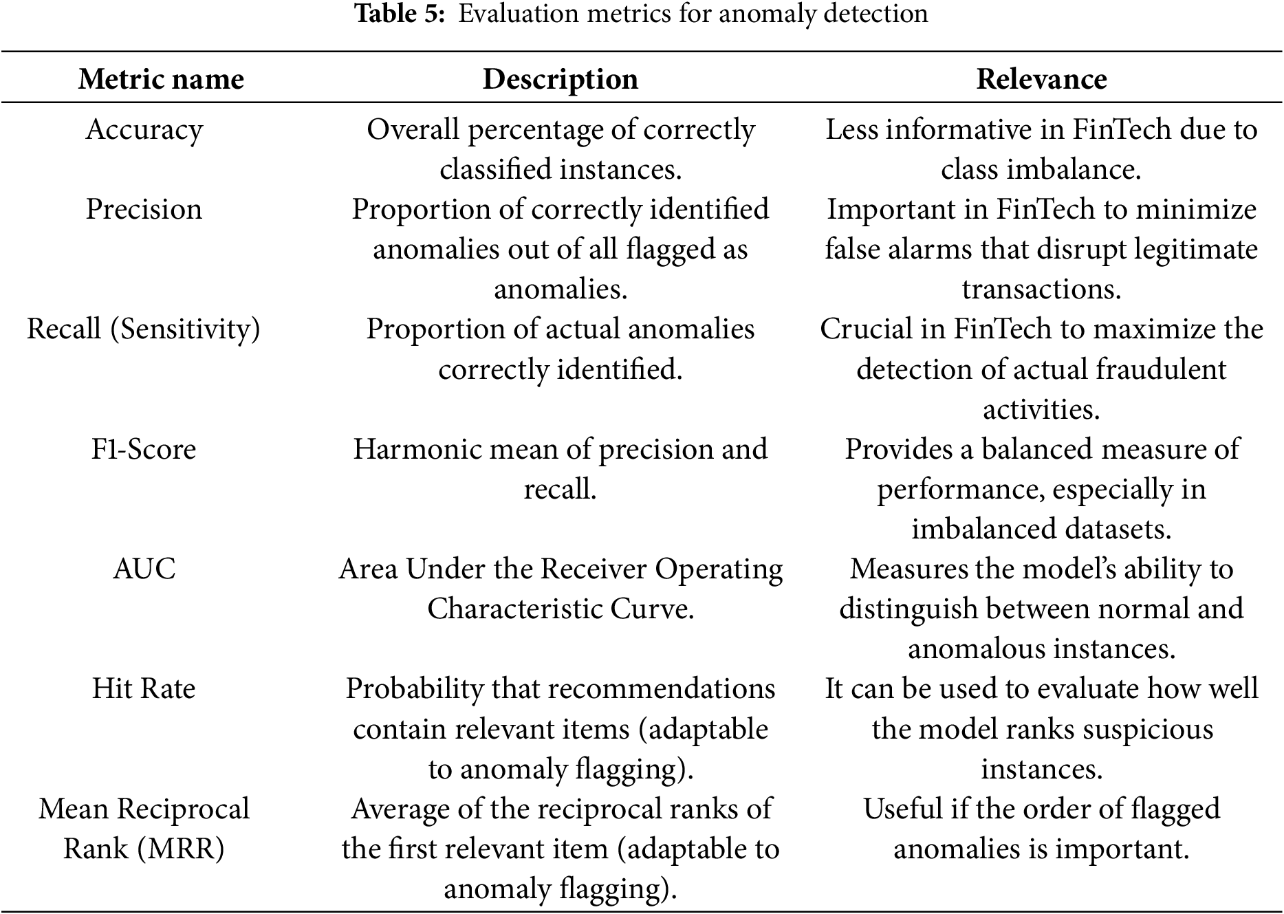
6.3 Metrics for Anomaly Detection

Evaluating the performance of anomaly detection models in the financial technology (FinTech) sector demands the use of carefully chosen context-sensitive metrics [28,73], as summarized in Table 5, to accurately capture a model’s ability to identify rare but potentially high-stakes anomalous events. Given the serious consequences of undetected fraud, financial manipulation, or operational failures, it is critical to select the right evaluation criteria. By integrating general performance metrics with domain-specific and time-aware evaluation methods, FinTech organizations can achieve a more comprehensive and actionable view of model effectiveness. This nuanced, multifaceted evaluation approach is essential for developing anomaly detection systems that are not only highly accurate, but also timely, interpretable, and aligned with real-world financial risk dynamics.

6.3.1 Standard Evaluation Metrics

Several commonly used metrics provide a foundation for assessing anomaly detection models:

1. Accuracy: As illustrated in Formula (28), this metric measures the overall percentage of correctly classified instances, both normal and anomalous. However, it can be misleading in highly imbalanced datasets (e.g., FinTech, where anomalies may represent less than 1% of transactions).

Accuracy=TP+TNTP+TN+FP+FN(28)

A model could achieve high accuracy simply by predicting all instances as normal while failing to detect any anomalies.

2. Precision: As illustrated in Formula (29), the proportion of correctly identified anomalies out of all instances flagged as anomalous. It reflects how trustworthy the model’s anomaly alerts are.

Precision=TPTP+FP(29)

3. Recall (Sensitivity): As illustrated in Formula (30), this metric measures the proportion of actual anomalies that the model successfully detects. High recall is critical in FinTech to minimize overlooked fraudulent or malicious activities.

Recall=TPTP+FN(30)

4. F1-Score: As illustrated in Formula (31), the harmonic mean of precision and recall, offering a balanced view of model performance, especially useful in imbalanced scenarios.

F1=2⋅Precision⋅RecallPrecision+Recall(31)

5. AUC-ROC (Area Under the Receiver Operating Characteristic Curve): Evaluates the model’s ability to distinguish between normal and anomalous classes across different threshold settings. A higher AUC (closer to 1) indicates better overall discriminative power.

6.3.2 Domain-Specific and Cost-Sensitive Metrics

In the FinTech domain, where errors carry financial and reputational consequences, additional tailored metrics are essential:

1. Cost-Sensitive Metric: As illustrated in Formula (32), this metric assign different weights to errors:

Cost=CFP⋅FP+CFN⋅FN(32)

where CFP and CFN represent the cost of false positives and false negatives, respectively. This approach helps align model performance with real-world financial impacts.

2. Ranking-Based Metric: Adapted from recommender systems [19,26] to prioritize anomalies:

•   Hit Rate @ k: Proportion of actual anomalies found in the top-k predicted results.

•   Mean Reciprocal Rank (MRR): Measures how early the first true anomaly appears in the ranked list, as illustrated in Formula (33):

MRR=1n∑i=1N1ranki(33)

6.3.3 Time-Series Evaluation Metrics

Given the temporal nature of financial data, time-aware metrics are critical:

1. Temporal Distance: Measures how close in time a predicted anomaly is to the actual one, as defined in Formula (34):

Temporal Distance=|timepred−timetrue|(34)

2. Total Detected in Range (TDIR): Counts how many true anomalies fall within a predefined window around the prediction.

3. Detection Accuracy in Range (DAIR): Ratio of true anomalies detected within the acceptable time window over total actual anomalies, as illustrated in Formula (35):

DAIR=Detected in rangeTotal true anomalies(35)

4. Weighted Metrics: Apply importance scores to detections, as illustrated in Formulas (36) and (37):

Weighted Precision=∑iwi⋅TPi∑iwi⋅(TPi+FPi)(36)

Weighted Recall=∑iwi⋅TPi∑iwi⋅(TPi+FNi)(37)

where wi is a weight based on contextual factors (e.g., time of day, risk level of the account).

7  Case Studies and Real-World Applications

7.1 GNNs for Anomaly Detection in Fintech

Numerous research studies and industrial deployments have demonstrated the strong efficacy of Graph Neural Networks (GNNs) in addressing anomaly detection challenges across a wide range of FinTech applications. Some of the most prominent use cases [40,74–76] include the detection of fraudulent transactions in credit card systems, e-commerce platforms, peer-to-peer payments, and digital wallets.

A notable example comes from NVIDIA [26], which developed an end-to-end AI pipeline that integrates GNN with XGBoost, achieving substantial improvements in fraud detection accuracy. In this hybrid architecture, GNNs are employed to learn latent representations of transaction graphs, capturing relationships between users, accounts, devices, and merchants. These embeddings are then passed to an XGBoost classifier, leveraging its strong gradient-boosted decision trees to refine anomaly predictions. Formally, if hi denotes the GNN-generated embedding for the transaction i, XGBoost predicts the fraud score yi via Formula (38):

yi=∑m=1Mfm(hi),fm∈ℱ(38)

where ℱ denotes the space of regression trees, and M is the number of trees.

In academic research, several advanced GNN models have been proposed to further enhance anomaly detection. For instance, CaT-GNN (Causal Temporal Graph Neural Network) [75] is designed to model both causal and temporal dependencies among financial transactions. By incorporating causal invariant learning, CaT-GNN seeks to identify features X and graph structures G that preserve the predictive relationship P(Y|do(X)) across different environments, reducing the risk of spurious correlations. Temporal dependencies are modeled using gated recurrent units (GRUs) over graph-structured data.

Similarly, Jump-Attentive GNN [76] introduces a jumping knowledge attention mechanism, where node representations are aggregated across different layers to allow the model to flexibly focus on graph neighborhoods of varying sizes. Given intermediate embeddings hi(l) in layer l, the final node representation is calculated as illustrated in Formula (39):

hifinal=∑l=1Lαlhi(l),∑l=1Lαl=1(39)

with αl being learnable attention weights that prioritize the most informative layers.

Another influential model is the Relational Graph Convolutional Network (RGCN) [45,77], which extends traditional GCNs to heterogeneous graphs where multiple node and edge types exist. In RGCNs, the message passing function is adapted to account for the type of edge r, so that the updated representation for node i in layer l+1 is given by Formula (40):

hi(l+1)=σ(∑r∈ℛ∑j∈𝒩r(i)1ci,rWr(l)hj(l)+W0(l)hi(l))(40)

where 𝒩r(i) denotes the neighbors of i under the relation r, Wr(l) are relation-specific weights, and ci,r is a normalization constant.

On the industry front, Alipay, one of the largest digital payment platforms worldwide, has successfully deployed heterogeneous GNNs [78] on a scale for fraud detection. Their system constructs massive transaction graphs, where nodes represent users, devices, IP addresses, and merchants, and edges represent transactions, logins, or behavioral similarities. By leveraging heterogeneous GNNs, Alipay’s models can detect subtle fraudulent patterns, such as coordinated money laundering schemes or device-sharing behaviors, that would be difficult to capture using traditional machine learning techniques. As illustrated in Formula (41), feature aggregation across heterogeneous node types is often implemented using attention mechanisms, where the importance score for neighbor type t is learned dynamically:

eti,j=LeakyReLU(a⊤[Wthi‖Wthj])(41)

where ∥ denotes concatenation, Wt are type-specific transformation matrices, and a is a learnable vector.

These examples collectively illustrate that the integration of advanced GNN architectures, often combined with traditional machine learning techniques like XGBoost, has become a leading paradigm for anomaly detection in FinTech. This enables real-time, scalable, and interpretable fraud detection systems in highly dynamic financial environments.

7.2 Integrating Feature Selection with GNNs in FinTech

The integration of Graph Neural Networks (GNNs) with feature selection has demonstrated significant potential in advancing anomaly detection across diverse domains. In financial transaction analysis, this synergy enhances fraud detection by filtering redundant or noisy attributes, enabling GNNs to capture relational and temporal dependencies more effectively [70]. In heterogeneous and dynamic graphs, feature selection aids in uncovering temporal patterns while reducing graph complexity, thereby improving scalability and adaptability of GNN-based models [71]. Recent work further highlights that feature-enhanced frameworks, especially when combined with contrastive learning, can align selected features with both local and global structural patterns, boosting anomaly detection accuracy [72]. Foundation models such as AnomalyGFM illustrate how feature selection supports zero-shot or few-shot detection, empowering GNNs to generalize effectively in data-scarce environments [69]. Together, these findings underscore the potential of integrating feature selection and GNNs to produce models that are more efficient, accurate, and interpretable for real-world applications in finance, cybersecurity, and other high-stakes domains.

Despite this progress, the FinTech domain still lacks extensive case studies explicitly validating such integration in operational settings. Hybrid feature selection frameworks are emerging that combine the efficiency of filter-based techniques with the adaptability of wrapper-based methods. Typically, filters such as mutual information ranking, chi-squared tests, and variance thresholding are used to prune irrelevant or weakly informative features, thereby reducing dimensionality and computational burden. Wrapper methods then iteratively refine feature subsets using GNN models as evaluators, with quality assessed through metrics such as Area Under the Curve (AUC), precision-recall, and F1-score. Embedding domain-specific constraints, such as transaction semantics, temporal dependencies, and regulatory requirements, into these pipelines could further enhance interpretability, transparency, and compliance in FinTech applications.

Formally, the hybrid feature selection objective can be expressed in Formula (42):

S∗=arg⁡maxS⊆F Score(GNN(XS,A))(42)

where S is a subset of the complete feature set F, XS represents node attributes restricted to S, A is the adjacency matrix, and Score(⋅) denotes a performance measure. By reducing feature space dimensionality while preserving essential structural and attribute information, such hybrid methods improve both anomaly detection accuracy and computational efficiency.

In addition to pre-processing, feature selection can also be embedded directly into model training. A promising approach leverages attention mechanisms, where feature importance scores αij are learned jointly with node representations. The feature-augmented message passing process is given by Formula (43):

hi′=∑j∈N(i)αijWhj,αij=exp⁡(LeakyReLU(a⊤[Whi∥Whj]))∑k∈N(i)exp⁡(LeakyReLU(a⊤[Whi∥Whk]))(43)

allowing the network to dynamically prioritize the most informative neighbors and features during training.

Applied to FinTech, these techniques are particularly valuable given the high dimensionality, heterogeneity, and dynamic nature of financial datasets. Financial graphs often encompass multiple entity types, customers, merchants, transactions, devices, with complex and evolving relationships. Feature selection helps mitigate overfitting, improves transparency, and strengthens robustness against adversarial manipulation, such as fraudsters injecting noise to obscure illicit behavior.

In summary, the synergistic integration of feature selection and GNN architectures represents a compelling yet underexplored research direction for anomaly detection in FinTech. By combining the dimensionality reduction and interpretability benefits of feature selection with the representational power of GNNs, future systems could achieve greater accuracy, efficiency, and resilience. Deepening this integration, while incorporating domain-specific constraints such as fraud patterns, transaction semantics, and regulatory requirements, would enable the development of robust, scalable, and explainable models. Such advancements are crucial for aligning anomaly detection pipelines with the operational, security, and compliance demands of modern financial ecosystems, while also fostering greater trust and transparency among institutions, regulators, and end-users.

8  Discussion

Integrating Graph Neural Networks (GNNs) with feature selection [69,70–72] in anomaly detection for FinTech applications offers significant promise, but it also introduces multiple challenges and limitations that must be addressed for practical deployment. Financial transaction data [9–11] are often sparse, with many accounts or users having only limited interaction histories. This sparsity reduces the ability of GNNs to learn robust node and edge representations, which is particularly problematic for detecting rare anomalies such as fraud, where signals are weak and distributed across large-scale networks. Scalability is another major concern: training and deploying GNNs over massive financial graphs is computationally expensive, and achieving real-time detection in production environments remains difficult. Class imbalance exacerbates these issues, as fraudulent or anomalous events are vastly outnumbered by legitimate transactions, causing models to become biased toward normal behavior and under-detect the critical minority class. Compounding this, the dynamic and adaptive nature of fraud requires models to be continuously retrained to capture new attack vectors, further straining computational and operational resources.

Beyond these data-centric and computational challenges, GNN models [79–81] also face structural and methodological limitations. The cold-start problem remains unsolved, as accounts or users with little transaction history offer minimal signals for reliable anomaly detection. Additionally, GNNs are vulnerable to adversarial attacks, where small perturbations to graph structures or node attributes can mislead models into misclassifications, raising serious concerns about the robustness of these systems in adversarial financial environments. Interpretability is another pressing challenge: GNNs often function as opaque “black boxes”, making it difficult to explain anomaly detection outcomes in a manner suitable for regulators, auditors, and business stakeholders. While feature selection can help mitigate this by reducing noise and focusing on relevant attributes, identifying meaningful features in highly complex financial graphs requires deep domain expertise and remains a non-trivial task.

To overcome these limitations, future research must prioritize the design of scalable and efficient GNN architectures [82–86] that can handle the scale and velocity of financial data streams in near real time. Interpretability should also be a core research direction, with explainable AI (XAI) approaches for GNNs [87–92] providing transparency into decision-making and fostering trust in regulated financial environments. Addressing class imbalance through cost-sensitive learning, anomaly oversampling, and graph-level augmentation strategies is critical to improving detection performance. The cold-start problem may be alleviated through transfer learning, graph pre-training, or meta-learning approaches that allow models to generalize from minimal user histories. Moreover, temporal and dynamic GNNs [71,93,94] represent a promising direction to capture evolving fraud tactics by modeling sequential dependencies and adapting to structural changes in financial transaction graphs.

Enhancing robustness is equally crucial: adversarial defense strategies must be developed to ensure that GNN-based fraud detection systems remain resilient under deliberate manipulation. Emerging research on agentic AI [95–97], autonomous AI systems with persistent goals, adaptive capabilities, and self-directed optimization, could further strengthen FinTech anomaly detection pipelines by enabling systems not only to respond to fraud, but also to anticipate and proactively adapt to new threats. Finally, semi-supervised and unsupervised learning paradigms [98–102] offer strong potential in domains where labeled fraud data are scarce, allowing models to leverage large volumes of unlabeled transaction data for more flexible anomaly detection.

In sum, the integration of GNNs and feature selection represents a powerful but still underexplored pathway to building anomaly detection systems in FinTech that are scalable, interpretable, and resilient. By advancing hybrid feature selection frameworks, robust GNN architectures, and adaptive learning paradigms, while embedding domain-specific knowledge such as transaction semantics and regulatory constraints, future systems can move closer to delivering anomaly detection solutions that are not only accurate, but also fair, transparent, and trustworthy in modern financial ecosystems.

9  Conclusion

This paper has explored the integration of Graph Neural Networks (GNNs) with feature selection techniques for anomaly detection in the FinTech sector. GNNs have emerged as a transformative tool for modeling and analyzing complex relational structures inherent in financial systems, making them well-suited for detecting anomalies such as fraudulent transactions, market manipulation, and irregular customer behavior. By capturing dependencies across entities and transactions, GNNs provide a holistic perspective on financial interactions that traditional machine learning methods often overlook.

When combined with feature selection, GNN-based models are able to focus on the most relevant attributes, thereby mitigating the challenges posed by high-dimensional financial data. Feature selection reduces noise, eliminates redundant variables, and improves both accuracy and computational efficiency. This dimensionality reduction is not only critical for improving detection performance but also enhances interpretability, an essential requirement in the FinTech domain, where regulatory compliance and transparency are as important as predictive power.

Recent advancements in agentic AI, characterized by systems capable of autonomous decision-making and proactive adaptation, present new opportunities for anomaly detection. Incorporating agentic AI into GNN-based frameworks allows anomaly detection models to transition from static pattern recognition to dynamic, context-aware systems. Such models can autonomously adapt to evolving fraud strategies, proactively identify emerging risks, and update detection mechanisms in near real-time. This capability significantly enhances the resilience of financial ecosystems, which are constantly exposed to adversarial behaviors and shifting regulatory landscapes.

Nevertheless, the integration of GNNs and feature selection introduces several pressing challenges. Data sparsity remains a significant obstacle, as financial transaction graphs are often incomplete or irregular. Scalability is another concern, given that financial datasets are massive and continuously growing in real time. Additionally, the interpretability of deep learning models remains problematic, with GNNs often criticized as black boxes. The adaptive tactics of fraudsters exacerbate these problems, forcing detection systems to contend with an adversarial environment that is both highly dynamic and strategically deceptive. The cold start problem, where there are limited data for new users or accounts, further complicates anomaly detection.

Despite these challenges, the potential benefits are considerable. Integrating feature selection with GNNs can yield models that are not only more accurate and computationally efficient but also adaptive and interpretable. Future research should focus on the development of scalable GNN architectures tailored to large-scale financial graphs, graph-specific feature selection algorithms to extract meaningful patterns, and agentic AI mechanisms to ensure autonomous adaptability and real-time responsiveness. Addressing these research directions will be crucial to creating next-generation anomaly detection frameworks.

Ultimately, the synergy between GNNs and feature selection holds the promise of transforming anomaly detection in FinTech. By improving accuracy, adaptability, and transparency, such systems can significantly strengthen defenses against fraud, increase trust, and improve the resilience of global financial infrastructures. This integrated approach is poised to become a cornerstone of proactive risk management and sustainable innovation in the financial industry.

Acknowledgement: We would like to thank Suan Sunandha Rajabhat University, Thailand for the support of time and facilities for this study.

Funding Statement: This work is jointly supported by Ho Chi Minh City Open University, Vietnam under grant number E2024.02.1CD and Suan Sunandha Rajabhat University, Thailand.

Author Contributions: The authors confirm contribution to the paper as follows: study conception and design, collection, analysis and interpretation of results, draft manuscript preparation: Nghia Dinh. Review paper: Viet-Tuan Le, Kiet Tran-Trung, Bay Nguyen Van, Vinh Truong Hoang, Kittikhun Meethongjan. All authors reviewed the results and approved the final version of the manuscript.

Availability of Data and Materials: The data that support the findings of this study are available from the corresponding author, upon reasonable request.

Ethics Approval: Not applicable.

Conflicts of Interest: The authors declare no conflicts of interest to report regarding the present study.

References

1. Tanis JH, Giannella C, Mariano AV. Introduction to graph neural networks: a starting point for machine learning engineers. arXiv:2412.19419. 2025. [Google Scholar]

2. Serrano W. Fintech model: the random neural network with genetic algorithm. Procedia Comput Sci. 2018;126(1):537–46. doi:10.1016/j.procs.2018.07.288. [Google Scholar] [CrossRef]

3. Khemani B, Patil S, Kotecha K, Tanwar S. A review of graph neural networks: concepts, architectures, techniques, challenges, datasets, applications, and future directions. J Big Data. 2024;11(1):18. doi:10.1186/s40537-023-00876-4. [Google Scholar] [CrossRef]

4. Liu Z, Yu H, Luo X. Federated graph anomaly detection via disentangled representation learning. In: Proceedings of the ACM Web Conference 2025 (WWW’25); 2025 Apr 28–May 2; Sydney, NSW, Australia; 2025. p. 1216–24. doi:10.1145/3696410.3714567. [Google Scholar] [CrossRef]

5. Htun HH, Biehl M, Petkov N. Survey of feature selection and extraction techniques for stock market prediction. Financ Innov. 2023;9(1):26. doi:10.1186/s40854-022-00441-7. [Google Scholar] [PubMed] [CrossRef]

6. Li K, Wang F, Yang L, Liu R. Deep feature screening: feature selection for ultra high-dimensional data via deep neural networks. Amsterdam, The Netherlands: Elsevier; 2023. [Google Scholar]

7. Palakurti NR. Challenges and future directions in anomaly detection. In: Whig P, Sharma S, Sharma S, Jain A, Yathiraju N, editors. Practical applications of data processing, algorithms, and modeling. Hershey, PA, USA: IGI Global; 2024. p. 269–84. doi:10.4018/979-8-3693-2909-2.ch020. [Google Scholar] [CrossRef]

8. Ren J, Tang T, Jia H, Fayek H, Li X, Ma S, et al. Foundation models for anomaly detection: vision and challenges. arXiv:2502.06911. 2025. [Google Scholar]

9. Una BK, Prabowo HY. FinTech lending fraud prevention strategy: a case study. J Contemp Account. 2022;4(1):37–52. doi:10.20885/jca.vol4.iss1.art4. [Google Scholar] [CrossRef]

10. Stojanović B, Božić J, Hofer-Schmitz K, Nahrgang K, Weber A, Badii A, et al. Follow the trail: machine learning for fraud detection in FinTech applications. Sensors. 2021;21(5):1594. doi:10.3390/s21051594. [Google Scholar] [PubMed] [CrossRef]

11. Garg Y, Kadian K, Mahajan V, Somya. Unmasking financial deception: leveraging machine learning for risk analysis and fraud detection in financial markets. In: 2024 IEEE Region 10 Symposium (TENSYMP); 2024 Sep 27–29; New Delhi, India. p. 1–6. doi:10.1109/TENSYMP61132.2024.10752159. [Google Scholar] [CrossRef]

12. Hao Y, Vand B, Delgado BM, Baldi S. Market manipulation in stock and power markets: a study of indicator-based monitoring and regulatory challenges. Energies. 2023;16(4):1894. doi:10.3390/en16041894. [Google Scholar] [CrossRef]

13. Dou Y, Liu Z, Sun L, Deng Y, Peng H, Yu PS. Enhancing graph neural network-based fraud detectors against camouflaged fraudsters. In: Proceedings of the 29th ACM International Conference on Information & Knowledge Management; 2020 Oct 19–23; Online. p. 315–24. [Google Scholar]

14. Khan Z, Khan Z, Lee BG, Kim HK, Jeon M. Graph neural networks based framework to analyze social media platforms for malicious user detection. Appl Soft Comput. 2024;155(C):111416. doi:10.1016/j.asoc.2024.111416. [Google Scholar] [CrossRef]

15. Teng X, Lin YR, Wen X. Anomaly detection in dynamic networks using multi-view time-series hypersphere learning. In: Proceedings of the 2017 ACM on Conference on Information and Knowledge Management; 2017 Nov 6–10; Singapore. p. 827–36. [Google Scholar]

16. Hayawi K, Saha S, Masud MM, Mathew SS, Kaosar M. Social media bot detection with deep learning methods: a systematic review. Neural Comput Appl. 2023;35(12):8903–18. doi:10.1007/s00521-023-08352-z. [Google Scholar] [CrossRef]

17. Klicpera J, Becker F, Günnemann S. Gemnet: universal directional graph neural networks for molecules. In: Proceedings of the 35th International Conference on Neural Information Processing Systems; 2021 Dec 6–14; Online. p. 6790–802. [Google Scholar]

18. Jia X, Jiang M, Dong Y, Zhu F, Lin H, Xin Y, et al. Multimodal heterogeneous graph attention network. Neural Comput Appl. 2023;35(4):3357–72. doi:10.1007/s00521-022-07862-6. [Google Scholar] [CrossRef]

19. Pucci A, Gori M, Hagenbuchner M, Scarselli F, Tsoi A. Investigation into the application of graph neural networks to large-scale recommender systems. Syst Sci. 2006;32(4):17–26. doi:10.1109/tnn.2008.2005141. [Google Scholar] [CrossRef]

20. Defferrard M, Bresson X, Vandergheynst P. Convolutional neural networks on graphs with fast localized spectral filtering. In: Lee D, Sugiyama M, Luxburg U, Guyon I, Garnett R, editors. Advances in neural information processing systems. Red Hook, NY, USA:Curran Associates, Inc.; 2016. Vol. 29. [Google Scholar]

21. Brody S, Alon U, Yahav E. How attentive are graph attention networks? arXiv:2105.14491. 2021. [Google Scholar]

22. Nuanmeesri S. Feature selection for analyzing data errors toward development of household big data at the sub-district level using multi-layer perceptron neural network. Int J Interact Mob Technol. 2022;16(5):121–38. doi:10.3991/ijim.v16i05.22523. [Google Scholar] [CrossRef]

23. Oh J, Cho K, Bruna J. Advancing graphsage with a data-driven node sampling. arXiv:1904.12935. 2019. [Google Scholar]

24. Chen S, Song X, Theodore V, Liu H. Deal: distributed End-to-End GNN inference for all nodes. arXiv:2503.02960. 2025. [Google Scholar]

25. Gupta A, Matta P, Pant B. Graph neural network: current state of Art, challenges and applications. Mater Today Proc. 2021;46(4):10927–32. doi:10.1016/j.matpr.2021.01.950. [Google Scholar] [CrossRef]

26. Wu S, Sun F, Zhang W, Xie X, Cui B. Graph neural networks in recommender systems: a survey. ACM Comput Surveys. 2022;55(5):1–37. doi:10.1145/3535101. [Google Scholar] [CrossRef]

27. Malla AM, Banka AA. Comprehensive review of graph neural networks: challenges, classification, architectures, applications, and potential utility in bioinformatics. Expert Syst. 2025;42(8):e70091. doi:10.1111/exsy.70091. [Google Scholar] [CrossRef]

28. Zhang H, Wu B, Yuan X, Pan S, Tong H, Pei J. Trustworthy graph neural networks: aspects, methods, and trends. Proc IEEE. 2024;112(2):97–139. doi:10.1109/jproc.2024.3369017. [Google Scholar] [CrossRef]

29. Zhang Q, Zhang Y, Yao X, Li S, Zhang C, Liu P. A dynamic attributes-driven graph attention network modeling on behavioral finance for stock prediction. ACM Trans Knowl Discov Data. 2023;18(1):1–29. doi:10.1145/3611311. [Google Scholar] [CrossRef]

30. Cheng H, Wang K, Tan X. A link prediction method for Chinese financial event knowledge graph based on graph attention networks and convolutional neural networks. Eng Appl Artif Intell. 2024;138(3):109361. doi:10.1016/j.engappai.2024.109361. [Google Scholar] [CrossRef]

31. Zhang W, Chen Z, Miao J, Liu X. Research on graph neural network in stock market. Procedia Comput Sci. 2022;214(7):786–92. doi:10.1016/j.procs.2022.11.242. [Google Scholar] [CrossRef]

32. Wang D, Zhang Z, Zhao Y, Huang K, Kang Y, Zhou J. Financial default prediction via motif-preserving graph neural network with curriculum learning. In: Proceedings of the 29th ACM SIGKDD Conference on Knowledge Discovery and Data Mining; 2023 Aug 6–10; Long Beach, CA, USA. p. 2233–42. [Google Scholar]

33. Xiao L, Yang X, Yang X. A graph neural network-based bearing fault detection method. Sci Rep. 2023;13(1):5286. [Google Scholar] [PubMed]

34. Skillicorn DB. Detecting anomalies in graphs. In: IEEE International Conference on Intelligence and Security Informatics; 2007 May 23–24; New Brunswick, NJ, USA. p. 209–16. [Google Scholar]

35. Lamichhane PB, Eberle W. Anomaly detection in graph structured data: a survey. arXiv:2405.06172. 2024. [Google Scholar]

36. Ma X, Wu J, Xue S, Yang J, Zhou C, Sheng QZ, et al. A comprehensive survey on graph anomaly detection with deep learning. IEEE Trans Knowl Data Eng. 2021;35(12):12012–38. doi:10.1109/tkde.2021.3118815. [Google Scholar] [CrossRef]

37. Noble CC, Cook DJ. Graph-based anomaly detection. In: Proceedings of the Ninth ACM SIGKDD International Conference on Knowledge Discovery and Data Mining; 2003 Aug 24–27; Washington, DC, USA. p. 631–6. [Google Scholar]

38. Wu N, Zhao Y, Dong H, Xi K, Yu W, Wang W. Federated graph anomaly detection through contrastive learning with global negative Pairs. In: Proceedings of the AAAI Conference on Artificial Intelligence. Vol. 39. Palo Alto, CA, USA: AAAI; 2025. p. 21554–62. [Google Scholar]

39. You Y, Chen T, Sui Y, Chen T, Wang Z, Shen Y. Graph contrastive learning with augmentations. Adv Neural Inf Process Syst. 2020;33:5812–23. [Google Scholar]

40. Yu H, Liu W, Zhu N, Li P, Luo X. IN-GFD: an interpretable graph fraud detection model for spam reviews. IEEE Trans Artif Intell. 2024;5(10):5325–39. doi:10.1109/tai.2024.3420262. [Google Scholar] [CrossRef]

41. Kim H, Lee BS, Shin WY, Lim S. Graph anomaly detection with graph neural networks: current status and challenges. IEEE Access. 2022;10(9):111820–9. doi:10.1109/access.2022.3211306. [Google Scholar] [CrossRef]

42. Becker L. Anomaly detection in E-commerce platforms via graph neural networks. Asia Pacific Econ Manag Rev. 2025;2(2):1–10. doi:10.62177/apemr.v2i2.208. [Google Scholar] [CrossRef]

43. Liao W, Zeng B, Liu J, Wei P, Cheng X, Zhang W. Multi-level graph neural network for text sentiment analysis. Comput Electr Eng. 2021;92:107096. [Google Scholar]

44. Yang X, Ma H, Wang M. Research on rumor detection based on a graph attention network with temporal features. Int J Data Warehous Min (IJDWM). 2023;19(2):1–17. doi:10.4018/ijdwm.319342. [Google Scholar] [CrossRef]

45. Schlichtkrull M, Kipf TN, Bloem P, Van Den Berg R, Titov I, Welling M. Modeling relational data with graph convolutional networks. In: European Semantic Web Conference. Cham, Switzerland: Springer; 2018. p. 593–607. [Google Scholar]

46. Yang X, Deng C, Liu T, Tao D. Heterogeneous graph attention network for unsupervised multiple-target domain adaptation. IEEE Trans Pattern Anal Mach Intell. 2020;44(4):1992–2003. doi:10.1109/tpami.2020.3026079. [Google Scholar] [PubMed] [CrossRef]

47. Chicchi L, Giambagli L, Buffoni L, Marino R, Fanelli D. Complex recurrent spectral network. Chaos Solitons Fractals. 2024;184:114998. [Google Scholar]

48. Cao D, Wang Y, Duan J, Zhang C, Zhu X, Huang C, et al. Spectral temporal graph neural network for multivariate time-series forecasting. Adv Neural Inf Process Syst. 2020;33:17766–78. [Google Scholar]

49. Ding Y, Zhang ZL, Zhao XF, Cai W, He F, Cai YM, et al. Deep hybrid: multi-graph neural network collaboration for hyperspectral image classification. Defence Technol. 2023;23(4):164–76. doi:10.1016/j.dt.2022.02.007. [Google Scholar] [CrossRef]

50. Ma Y, Hao J, Yang Y, Li H, Jin J, Chen G. Spectral-based graph convolutional network for directed graphs. arXiv:1907.08990. 2019. [Google Scholar]

51. Liu B, Wu L. Graph neural networks in natural language processing. In: Graph neural networks: foundations, frontiers, and applications. Cham, Switzerland: Springer; 2022. p. 463–81. doi:10.1007/978-981-16-6054-2_21. [Google Scholar] [CrossRef]

52. Wang Y. Advances in spatiotemporal graph neural network prediction research. Int J Digital Earth. 2023;16(1):2034–66. [Google Scholar]

53. Wu Z, Pan S, Long G, Jiang J, Chang X, Zhang C. Connecting the dots: multivariate time series forecasting with graph neural networks. In: Proceedings of the 26th ACM SIGKDD International Conference on Knowledge Discovery & Data Mining; 2020 Jul 6–10; Online. p. 753–63. [Google Scholar]

54. Liu Z, Luo Y, Duan M. Macroeconomic factors, industrial enterprises, and debt default prediction: based on the VAR-GRU model. Amsterdam, The Netherlands: Elsevier; 2025. [Google Scholar]

55. Hamilton W, Ying Z, Leskovec J. Inductive representation learning on large graphs. In: Proceedings of the Neural Information Processing Systems 30 (NIPS 2017); 2017 Dec 4–9; Long Beach, CA, USA. [Google Scholar]

56. Chen J, Ma T, Xiao C. FastGCN: fast learning with graph convolutional networks via importance sampling. arXiv:1801.10247. 2018. [Google Scholar]

57. Pareja A, Domeniconi G, Chen J, Ma T, Suzumura T, Kanezashi H, et al. Evolvegcn: evolving graph convolutional networks for dynamic graphs. In: Proceedings of the AAAI Conference on Artificial Intelligence. vol. 34. Palo Alto, CA, USA: AAAI; 2020. p. 5363–70. [Google Scholar]

58. Xu D, Ruan C, Korpeoglu E, Kumar S, Achan K. Inductive representation learning on temporal graphs. arXiv:2002.07962. 2020. [Google Scholar]

59. Sankar A, Wu Y, Gou L, Zhang W, Yang H. Dysat: deep neural representation learning on dynamic graphs via self-attention networks. In: Proceedings of the 13th International Conference on Web Search and Data Mining; 2020 Feb 3–7; Houston, TX, USA. p. 519–27. [Google Scholar]

60. Bolón-Canedo V, Sánchez-Maroño N, Alonso-Betanzos A. Feature selection for high-dimensional data. Progress Artif Intell. 2016;5(2):65–75. doi:10.1007/s13748-015-0080-y. [Google Scholar] [CrossRef]

61. Theng D, Bhoyar KK. Feature selection techniques for machine learning: a survey of more than two decades of research. Knowl Inf Syst. 2024;66(3):1575–637. doi:10.1007/s10115-023-02010-5. [Google Scholar] [CrossRef]

62. Li J, Cheng K, Wang S, Morstatter F, Trevino RP, Tang J, et al. Feature selection: a data perspective. ACM Comput Surveys (CSUR). 2017;50(6):1–45. doi:10.1145/3136625. [Google Scholar] [CrossRef]

63. Pang N, Xia X. Distributed conditional feature screening via pearson partial correlation with FDR contro. arXiv:2403.05792. 2024. [Google Scholar]

64. Fira M, Goras L, Costin HN. Evaluating sparse feature selection methods: a theoretical and empirical perspective. Appl Sci. 2025;15(7):3752. doi:10.3390/app15073752. [Google Scholar] [CrossRef]

65. Guyon I, Elisseeff A. An introduction to variable and feature selection. J Machine Learn Res. 2003;3:1157–82. [Google Scholar]

66. Yuan X, Yuan J, Jiang T, Ain QU. Integrated long-term stock selection models based on feature selection and machine learning algorithms for China stock market. IEEE Access. 2020;8:22672–85. doi:10.1109/access.2020.2969293. [Google Scholar] [CrossRef]

67. Min Y, Ye M, Tian L, Jian Y, Zhu C, Yang S. Unsupervised feature selection via multi-step markov probability relationship. Neurocomputing. 2021;453(3):241–53. doi:10.1016/j.neucom.2021.04.073. [Google Scholar] [CrossRef]

68. Jachymczyk U, Knap P. Review of feature selection methods for Predictive Maintenance Systems. Industry 4.0. 2024;9(3):97–100. [Google Scholar]

69. Qiao H, Niu C, Chen L, Pang G. AnomalyGFM: graph foundation model for zero/few-shot anomaly detection. In: Proceedings of the 31st ACM SIGKDD Conference on Knowledge Discovery and Data Mining; 2025 Aug 3–7; Toronto, ON, Canada. p. 2326–37. [Google Scholar]

70. Pei Y, Lyu F, Van Ipenburg W, Pechenizkiy M. Subgraph anomaly detection in financial transaction networks. In: Proceedings of the First ACM International Conference on AI in Finance; 2020 Oct 15–16; New York, NY, USA. p. 1–8. [Google Scholar]

71. Liu J, Wang Y, Wang F. Temporal patterns discovery of evolving graphs for graph neural network (GNN)-based anomaly detection in heterogeneous [Internet]. 2025 [cited 2025 Apr 19]. Available from: https://jisis.org/wp-content/uploads/2022/11/jisis-2022-vol12-no1-05.pdf. [Google Scholar]

72. Lei Z, Pu P. Graph anomaly detection framework based on feature enhancement and contrastive learning. In: International Conference on Image Processing and Artificial Intelligence (ICIPAl 2024). Vol. 13213. Bellingham, WA, USA: SPIE; 2024. p. 564–9. [Google Scholar]

73. Kim GY, Lim SM, Euom IC. A study on performance metrics for anomaly detection based on industrial control system operation data. Electronics. 2022;11(8):1213. doi:10.3390/electronics11081213. [Google Scholar] [CrossRef]

74. Choi J, Kim H, Whang JJ. Unveiling the threat of fraud gangs to graph neural networks: multi-target graph injection attacks against GNN-based fraud detectors. In: Proceedings of the AAAI Conference on Artificial Intelligence. Vol. 39. Palo Alto, CA, USA: AAAI; 2025. p. 16028–36. [Google Scholar]

75. Alarfaj FK, Shahzadi S. Enhancing fraud detection in banking with deep learning: graph neural networks and autoencoders for real-time credit card fraud prevention. IEEE Access. 2025;13:20633–46. doi:10.1109/access.2024.3466288. [Google Scholar] [CrossRef]

76. Cheng D, Wang X, Zhang Y, Zhang L. Graph neural network for fraud detection via spatial-temporal attention. IEEE Trans Knowl Data Eng. 2020;34(8):3800–13. doi:10.1109/tkde.2020.3025588. [Google Scholar] [CrossRef]

77. Motie S, Raahemi B. Financial fraud detection using graph neural networks: a systematic review. Expert Syst Appl. 2024;240(3):122156. doi:10.1016/j.eswa.2023.122156. [Google Scholar] [CrossRef]

78. Liu Z, Chen C, Yang X, Zhou J, Li X, Song L. Heterogeneous graph neural networks for malicious account detection. In: Proceedings of the 27th ACM international Conference on Information and Knowledge Management; 2018 Oct 22–26; Torino, Italy. p. 2077–85. [Google Scholar]

79. Pillai V. Anomaly detection for innovators: transforming data into breakthroughs. Mumbai, India: Libertatem Media Private Limited; 2022. [Google Scholar]

80. Reiss T, Kour G, Zwerdling N, Anaby-Tavor A, Hoshen Y. From zero to hero: cold-start anomaly detection. arXiv:2405.20341. 2024. [Google Scholar]

81. Ma X, Li R, Liu F, Ding K, Yang J, Wu J. Graph anomaly detection with few labels: a data-centric approach. In: Proceedings of the 30th ACM SIGKDD Conference on Knowledge Discovery and Data Mining; 2024 Aug 25–29; Barcelona, Spain. p. 2153–64. [Google Scholar]

82. Dara S, Srinivasulu C, Babu CM, Ravuri A, Paruchuri T, Kilak AS, et al. Context-Aware auto-encoded graph neural model for dynamic question generation using NLP. ACM Trans Asian Low Resour Lang Inf Process. 2023;124:312. doi:10.1145/3626317. [Google Scholar] [CrossRef]

83. Liang F, Qian C, Yu W, Griffith D, Golmie N. Survey of graph neural networks and applications. Wirel Commun Mob Comput. 2022;2022(1):9261537. doi:10.1155/2022/9261537. [Google Scholar] [CrossRef]

84. Cheng D, Zou Y, Xiang S, Jiang C. Graph neural networks for financial fraud detection: a review. Front Comput Sci. 2025;19(9):199609. doi:10.1007/s11704-024-40474-y. [Google Scholar] [CrossRef]

85. Tjoa E, Guan C. A survey on explainable artificial intelligence (XAItoward medical XAI. IEEE Trans Neural Netw Learn Syst. 2021;32(11):4793–813. doi:10.1109/tnnls.2020.3027314. [Google Scholar] [PubMed] [CrossRef]

86. Guidotti R, Monreale A, Ruggieri S, Turini F, Giannotti F, Pedreschi D. A survey of methods for explaining black box models. ACM Comput Surv. 2018;51(5):1–42. doi:10.1145/3236009. [Google Scholar] [CrossRef]

87. Arrieta AB, Díaz-Rodríguez N, Del Ser J, Bennetot A, Tabik S, Barbado A, et al. Explainable Artificial Intelligence (XAIconcepts, taxonomies, opportunities and challenges toward responsible AI. Inf Fusion. 2020;58(3):82–115. doi:10.1016/j.inffus.2019.12.012. [Google Scholar] [CrossRef]

88. Jaeger M, Krügel S, Marinelli D, Papenbrock J, Schwendner P. Interpretable machine learning for diversified portfolio construction. J Financial Data Sci. 2021;3(3):31–51. doi:10.3905/jfds.2021.1.066. [Google Scholar] [CrossRef]

89. Du M, Liu N, Hu X. Techniques for interpretable machine learning. Commun ACM. 2019;63(1):68–77. doi:10.1145/3359786. [Google Scholar] [CrossRef]

90. Ali S, Abuhmed T, El-Sappagh S, Muhammad K, Alonso-Moral JM, Confalonieri R, et al. Explainable artificial intelligence (XAIwhat we know and what is left to attain trustworthy artificial intelligence. Inf Fusion. 2023;99(3):101805. doi:10.1016/j.inffus.2023.101805. [Google Scholar] [CrossRef]

91. Lan S, Ma Y, Huang W, Wang W, Yang H, Li P. DSTAGNN: dynamic spatial-temporal aware graph neural network for traffic flow forecasting. In: Proceedings of the 39th International Conference on Machine Learning (ICML). Vol. 162. Westminster, UK: PMLR; 2022. p. 11906–17. [Google Scholar]

92. Guo S, Lin Y, Feng N, Song C, Wan H. Attention based spatial-temporal graph convolutional networks for traffic flow forecasting. In: Proceedings of the AAAI Conference on Artificial Intelligence. Vol. 33. Palo Alto, CA, USA: AAAI; 2019. p. 922–9. [Google Scholar]

93. Acharya DB, Kuppan K, Divya B. Agentic AI: autonomous intelligence for complex goals-a comprehensive survey. IEEE Access. 2025;13(2):18912–36. doi:10.1109/access.2025.3532853. [Google Scholar] [CrossRef]

94. Han X, Wang N, Che S, Yang H, Zhang K, Xu SX. Enhancing investment analysis: optimizing AI-Agent collaboration in financial research. In: Proceedings of the 5th ACM International Conference on AI in Finance; 2024 Aug 14–18; New York NY, USA. p. 538–46. [Google Scholar]

95. Hughes L, Dwivedi YK, Malik T, Shawosh M, Albashrawi MA, Jeon I, et al. AI agents and agentic systems: a multi-expert analysis. J Comput Inf Syst. 2025;65(4):489–517. doi:10.1080/08874417.2025.2483832. [Google Scholar] [CrossRef]

96. Villa-Pérez ME, Alvarez-Carmona MA, Loyola-González O, Medina-Pérez MA, Velazco-Rossell JC, Choo KKR. Semi-supervised anomaly detection algorithms: a comparative summary and future research directions. Knowl Based Syst. 2021;218(3):106878. doi:10.1016/j.knosys.2021.106878. [Google Scholar] [CrossRef]

97. Wang D, Lin J, Cui P, Jia Q, Wang Z, Fang Y, et al. A semi-supervised graph attentive network for financial fraud detection. In: 2019 IEEE International Conference on Data Mining (ICDM); 2019 Nov 8–11; Beijing, China. p. 598–607. [Google Scholar]

98. Qiao H, Wen Q, Li X, Lim EP, Pang G. Generative semi-supervised graph anomaly detection. Adv Neural Inf Process Syst. 2024;37:4660–88. [Google Scholar]

99. Lee CH, Lee K. Semi-supervised anomaly detection algorithm based on KL divergence (SAD-KL). In: Anomaly detection and imaging with X-rays (ADIX) VIII. Vol. 12531. Bellingham, WA, USA: SPIE; 2023. p. 118–23. doi:10.1109/access.2021.3120710. [Google Scholar] [CrossRef]

100. Cui Y, Liu Z, Lian S. A survey on unsupervised anomaly detection algorithms for industrial images. IEEE Access. 2023;11:55297–315. doi:10.1109/access.2023.3282993. [Google Scholar] [CrossRef]

101. Cao Y, Xiang H, Zhang H, Zhu Y, Ting KM. Anomaly detection based on isolation mechanisms: a survey. arXiv:2403.10802. 2024. [Google Scholar]

102. Alvarez M, Verdier JC, Nkashama DK, Frappier M, Tardif PM, Kabanza F. A revealing large-scale evaluation of unsupervised anomaly detection algorithms. arXiv:2204.09825. 2022. [Google Scholar]