An Improved Forest Fire Detection Model Using Audio Classification and Machine Learning

1  Introduction

Forest and land fires are among the leading causes of environmental degradation, contributing significantly to climate change and potentially impeding progress towards Sustainable Development Goal 13 (Climate Action). The increasing frequency and intensity of these fires are driven by rising global temperatures, exploitative land clearing practices by corporations, and irresponsible human activities [1,2]. In addition, the negative impact of fires is a threat to economic losses and the safety of residents living in the surrounding area [3]. Fires are characterized by sudden onset, difficulty in extinguishment, and long duration. Therefore, understanding the behavior and spread of fires is important for effective early detection and monitoring.

A central component of fire detection and monitoring is data analysis, which involves processing and interpreting multi-source data, including satellite imagery, meteorological inputs, and field-based sensors [4]. Data analysis techniques can be carried out by image processing [5], statistical analysis [6], Machine Learning (ML) [7,8], hotspot identification and anomaly detection [9]. In addition, it can provide accurate information for fire management, including early fire detection [10].

Traditionally, fire detection has relied on satellite-based hotspot identification, where elevated surface temperatures are flagged as potential fire zones [11,12]. Hotspots are identified as areas with relatively higher surface temperatures compared to the surrounding areas based on the set temperature threshold. The number of hotspots monitored by satellite can be predicted as the potential for fires in the area [13]. However, not all hotspots can be categorized as potential fires, so investigation and validation are required for hotspots monitored by satellite via Remote Sensing (RS) [14]. According to Barmpoutis et al. [15], computer vision, RS, and ML technologies can offer efficient methods to detect and monitor forest fire events. Relevant studies agree that to detect forest fires quickly and efficiently, different algorithms were used, including the use of fuzzy algorithms to process wireless sensor datasets [16], bidirectional use of Long Short-Term Memory Network (LSTM) to detect fire through smoke [17], the use of Deep Learning (DL) based on Closed-Circuit Television (CCTV) images and weather data to make predictions about forest fire vulnerability [18].

Although image-based detection techniques generally maintain low false alarm rates and offer real-time responsiveness, they often struggle with feature extraction in complex, dynamic environments. DL approaches, particularly those leveraging artificial neural networks, have demonstrated improved feature extraction and robustness against environmental noise [19]. According to Lin et al. [20], fire prediction models can be broadly categorized into statistical models, which examine correlations between fires and environmental variables, and ML models, which uncover predictive patterns in data. However, as shown by Phelps and Woolford [21], both models exhibit similar performance when applied to small-scale, human-induced fires, suggesting that model selection should be context-sensitive and informed by field expertise.

Recent advancements have seen the deployment of DL-based fire detection models using CNNs and You Only Look Once (YOLO) object detection techniques [22,23], which are compatible with low-power devices but exhibit limitations in detection accuracy. Hybrid strategies that incorporate Spatial Pyramid Pooling Fast (SPPF) and Receptive Field Block (RFB) modules have been proposed to improve the detection performance of smoke and flame features [24], though at the cost of increased computational complexity.

While most fire detection research focuses on visual cues (smoke, flame, thermal anomalies), an emerging approach involves analyzing audio data captured from the fire environment [25]. Unlike general ambient sounds in forest environments such as bird chirping, insect buzzing, rainfall, or wind rustling, fire sounds exhibit distinctive acoustic patterns characterized by continuous crackling, popping, and roaring noises. These arise from the combustion of organic matter, where the release of gases and oxidation produces broadband, high-frequency bursts, and low-frequency flame roars. These auditory signatures present time–frequency characteristics distinct from meteorological noise, making them detectable through audio-based analysis. These sounds can be captured non-intrusively, even in obscured or low-visibility conditions. Additionally, microphones are lightweight, low-power, and cost-effective, making them well-suited for deployment in IoT-based early warning systems across large, rural areas.

CNNs are especially effective for this task, as they can learn spatial patterns from spectrograms, visual representations of the frequency spectrum of audio signals over time. The spectrogram captures temporal and spectral features of fire sounds, enabling CNNs to distinguish them from non-fire acoustic events, even under noisy conditions. Compared to traditional hand-crafted features, CNNs offer improved generalization by autonomously learning discriminative representations from complex acoustic scenes.

Therefore, this study proposes a novel land and forest fire detection technique based on audio data, allowing real-time identification of fire incidents based on direct sound recordings from the environment. The main contributions of this study are as follows:

•   Transforming an audio data stream into a spectrogram as a visual representation of the frequency spectrum over time.

•   Classifying spectrograms using a CNN algorithm data input to identify various types of sounds in the surrounding environment, such as wild animal sounds and weather conditions (rain and wind).

•   Evaluating the proposed model to ensure its effectiveness through accuracy metrics, F1-score, and confusion matrix analysis.

In the following, Section 2 discusses existing research related to fire detection; Section 3 presents the material and method. Section 4 provides results and discussion of the cases and methods discussed in this research, and finally, Section 5 concludes the overall results of the research.

2  Related Works

Audio-based classification has emerged as a promising method for environmental monitoring tasks, including anomaly detection and wildlife surveillance. However, its application in forest fire detection remains relatively underexplored, particularly in complex natural soundscapes. Recent advancements in fire detection technologies have focused predominantly on visual-based approaches, such as image and video analysis using CNN and object detection models like YOLO. These methods excel in clear weather or urban settings but suffer performance degradation under occlusion, nighttime conditions, or smoke-obstructed visibility. In forest environments, especially dense, remote, or poorly instrumented areas, visual cues are often unreliable or inaccessible, highlighting the need for alternative, robust modalities like acoustic sensing.

Prior works in environmental sound classification demonstrate the potential of audio as a reliable signal modality. Permana et al. [26] trained a CNN model to classify bird vocalizations under normal and disturbed (panic) states with an accuracy of 96.45%, suggesting that auditory cues can reflect critical environmental transitions. An audio classification experiment is also carried out by Huang et al. [27], on the dataset of fire sound recordings packaged in a data pipeline using ML. There are 3 stages in the data pipeline, namely audio preprocessing, feature extraction, and classification. All processes are carried out by Raspberry Pi 4 with 99% accuracy in identifying forest fires.

Sound is a complex signal with various audio features and classifications that have been widely used in various research fields. One of them is environmental sound monitoring [28,29], where sound classification is used to detect anomalies or identify certain events based on wildlife monitoring, vehicle sounds, alarms, etc. The sound signal processing technique begins with preprocessing to remove noise, amplitude normalization, and segmentation into frames [30]. The resulting audio frames are then used for analysis in the feature extraction process. The feature extraction results are used for classification using relevant models.

Research by Mohmmad and Sanampudi [31] used the Mel-Frequency Cepstral Coefficients (MFCC) [32], Mel-Spectrogram and Tonnetz feature extraction models to improve the classification accuracy of CNN models used for tree felling identification. The dataset consists of 4 classes (chainsaws, axes, manual saws, and other sounds from the forest environment) with 1200 samples for each class. The performance of the proposed model is very good, with an accuracy of 82% from 4800 audio samples. Representation and feature extraction have a significant impact on the performance of the ML model. Furthermore, their evaluations are primarily benchmark-focused, not tailored to the low-power, real-time constraints of forest-based IoT systems.

Approaches for fire prediction, rather than detection, are explored by Natekar et al. [33] to investigate prediction strategies using temporal fire data. They use previous weather conditions fed to Long Short-Term Memory (LSTM) and made predictions based on time-series forecasts using a Recurrent Neural Network (RNN) with an average accuracy of 94.77%. Huot et al. [34] use multivariate datasets, namely combining 2-D fire data from various variables such as topography, vegetation, weather, drought index, and population density from an area. By adopting an Artificial Neural Network (ANN), the spatial features of the data can predict the spread of forest and land fires. The results of ANN are compared with ML as a benchmark for developing a distribution model based on remote sensing data with a one-day waiting time. These models serve well in forecasting fire spread but are less useful for early real-time alerting.

Different approaches by Martinsson et al. [35] investigate whether the materials exposed to heat cause acoustic emissions during the heating, pyrolysis, and burning phases. The acoustic sound was collected and defined as acoustic data to be trained in detecting fire events using machine learning. Even though the results of testing on this laboratory scale produce a F1 score value of 98.4%. Although preliminary, this work provides a strong proof-of-concept for using acoustic emissions as direct indicators of combustion events.

Furthermore, Chu et al. [30] propose the mechanism of sound classification through extraction features using MFCC to convert sound into spectrograms. Experiment results show the classification accuracy on the Environmental Sound Classification (ESC-50) dataset was 97% while on the Urbansound8K Dataset was 92% after using augmentation data. Their results underscore the importance of representation learning in improving model generalization under diverse acoustic scenarios.

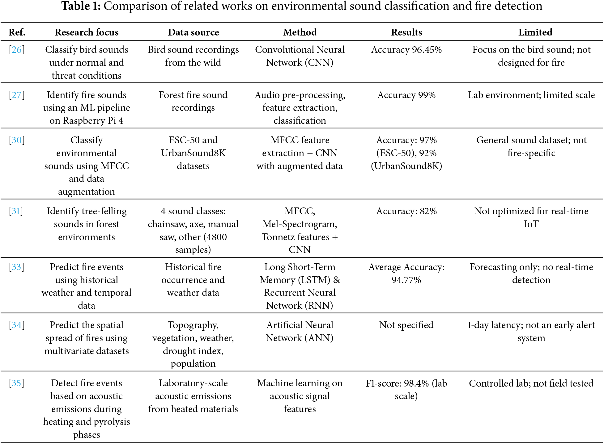
Despite these advancements, most prior works either focus on general environmental sounds or are limited to laboratory-scale fire scenarios. A clear research gap exists in developing robust, field-deployable acoustic models for fire detection in natural environments with overlapping sound sources. Furthermore, comparative studies on audio-based fire detection remain limited, particularly in evaluating performance under different thresholds and noise conditions. To clearly situate the present study within this context, Table 1 summarizes selected related works, highlighting their modalities, core methods, deployment settings, and performance metrics.

This study addresses this gap by proposing an audio-based forest fire detection system using CNNs applied to spectrogram representations of ambient sound. It uses mel-Spectrogram representations and evaluates multiple thresholds (k values) to control False Alarm Rates (FAR) under realistic deployment scenarios. Unlike prior studies, this work contributes a deployable architecture optimized for edge devices and performs ROC-based validation to measure operational trade-offs, ensuring the proposed system is lightweight, suitable for IoT deployment, and verified through comparative threshold analysis to optimize detection reliability while minimizing false alarm rates.

3  Material and Method

The proposed fire detection methodology follows a systematic pipeline. Raw audio data is first pre-processed and converted into a visual representation (mel-spectrogram). These spectrograms serve as input to a CNN, which is trained to perform binary classification (‘fire’ or ‘non-fire’). The model’s architecture is optimized for both high accuracy and computational efficiency. Data augmentation techniques are employed during training to enhance dataset variability and consistency, thereby boosting model generalization and accuracy.

3.1 Dataset Preparation

This study utilizes the publicly available multimodal dataset from [26], focusing exclusively on the audio modality to develop a robust forest fire detection framework. The dataset comprises audio recordings captured under diverse environmental conditions spanning various weather patterns, seasons, and times of day, and is explicitly labeled for binary classification: ‘fire’ and ‘non-fire.’ To improve ecological validity, audio contained the sound of fire mixed with noises related to climatic events, fauna, or even to unexpected events, as well as similar noises devoid of the sound of fire.

The audio samples were standardized to 5 s in duration and stored in 48 kHz/16-bit WAV format. The fire-class audio samples were primarily collected using field-grade Audio-Technica AT2020 condenser microphones, while non-fire sounds were sourced from established sound libraries including ESC-50 [27] and FSD50K [28], encompassing real-world non-fire environmental sounds. This multimodal collection strategy ensured heterogeneity and minimized sampling bias. To prepare the dataset for model training and evaluation, 2756 audio samples were selected: 1066 fire and 1690 non-fire.

3.1.1 Acoustic Properties

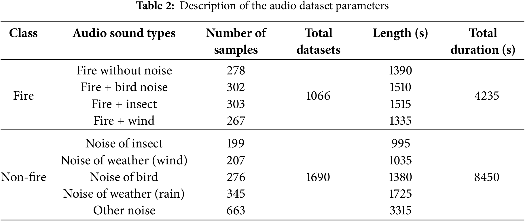
To enhance diversity and boost model generalizability, the fire and non-fire categories were divided into subtypes based on the dominant background noise characteristics. This approach allowed for focused model evaluation across different acoustic conditions. The dataset includes fire sounds with and without background noise (birds, insects, wind) and a variety of non-fire ambient sounds (isolated insects, weather, etc.). Table 2 provides a detailed overview of the parameters of the audio dataset.

3.1.2 Signal-to-Noise Ratio (SNR) Analysis

To assess the complexity and realism of the dataset, we conducted a statistical analysis of the Signal-to-Noise Ratio (SNR) for each sample. As visualized in Fig. 1 and detailed in Table 3, the SNR distribution reveals a dataset heavily skewed toward low SNR conditions. This distribution reveals a significant bias toward negative SNR values, with 84.7% of fire samples and 72.3% of non-fire samples having an SNR < 5 dB.

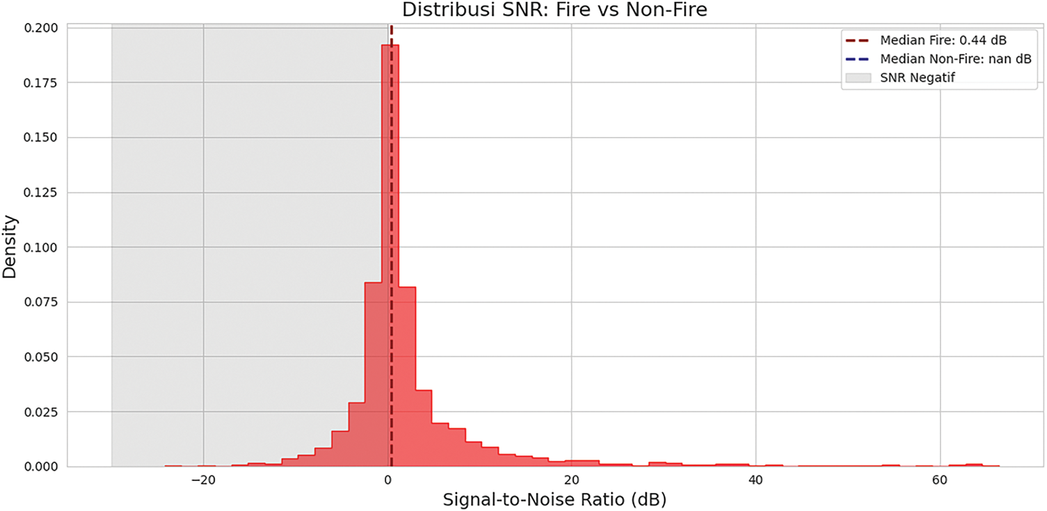
Figure 1: Distribution of SNR samples for fire vs. non-fire. The gray area marks the negative SNR region where the signal is weaker than the noise. The dotted lines indicate the median values for each class

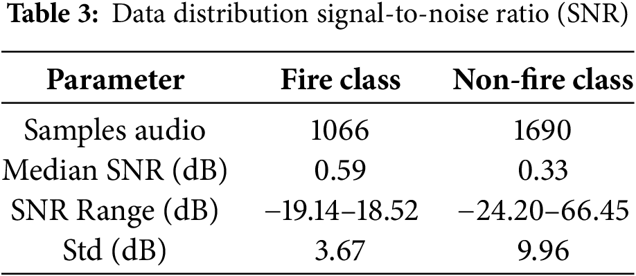
The median SNR values for the fire class (0.59 dB) and non-fire class (0.33 dB) indicate that more than half of the dataset is highly noisy (SNR < 1 dB). The extreme range −24.2–66.4 dB and high variance (σ = 9.96 dB for non-fire) reflect the diversity of acoustic conditions recorded in the environment. These noise characteristics pose a major challenge for fire detection in real-world environments and justify the specific augmentation approach proposed in Section 3.2.2.

3.2 Audio Pre-Processing and Feature Extraction

3.2.1 Spectrogram Conversion

To enhance model robustness in real-world acoustic environments, the raw fire and non-fire audio recordings (.wav) underwent systematic pre-processing and feature extraction before training. The end-to-end pipeline, shown in Fig. 2, transforms the input audio into mel-spectrograms, the final model input. This process is to train the prepared model from various audio capture angles. This is done to avoid uncertainty between similar audio, such as fire audio and rain audio, where, when listened to directly, there is a similarity in sound. To optimize the results of the training mode, the dataset downloaded from the source is required to go through a pre-reprocessing stage by reducing noise, amplitude normalization, and frame segmentation. To reduce noise on the audio signal, a pre-emphasis filter is applied using Eq. (1).

y(t)=x(t)−αx(t−1)(1)

where x is the original sound signal and x(t−1) is the signal that has passed through the high pass filter, while the filter coefficient is between 0.9 and 1 [30].

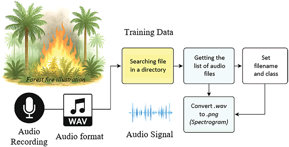
Figure 2: Preparation of training dataset

Amplitude normalization aims to equalize the volume of all audio in the dataset, ensuring the model is not biased towards high or low amplitudes. There are two methods: peak, which equalizes the maximum amplitude in decibels (dB), and Root Mean Square (RMS), which obtains the average energy of the audio signal. Audio signals fluctuate, so spectral analysis per time segment is required to detect accurate, unique patterns. Next, the magnitude is obtained from the number of frequencies in the audio signal through the Fast Fourier Transform (FFT) technique to produce a periodogram signal, namely identifying the dominant frequency cycle behavior of the time-series. In the feature extraction process, the audio signal frame is analyzed using the Short-Time Fourier Transform (STFT) technique to produce a frequency domain representation that can be further processed to obtain the required features.

This feature extraction method classifies environmental sound events based on the frequency-time representation. However, frame overlap will occur, resulting in a bell curve called the Hamming Window. This window function is used by the FFT to restore the waveform signal from 2 overlapping frames. To increase continuity between sound frames, the divided audio frame is multiplied by the Hamming Window to avoid signal discontinuity in the next Fourier transform. The Hamming Window is shown in Eq. (2), while the result of multiplying the sound frame by the Hamming Window is shown in Eq. (3).

W(t,α)={(1−α)−αxcos⁡(2πtT−1),0≤t≤T−10,otherwise(2)

Each frame y(t) is multiplied by this window to produce the smoothed output:

y′(t)=y(t)⋅W(t,α)(3)

where W(t,α) is the Hamming Window, t as the sampling point, T is the number of sampling points and generally the coefficient value is set at 0.46.

Mel scale spectrogram uses a Mel filter bank to reduce correlation between consecutive frequencies of the applied spectrogram. It has proven to be superior in exploiting non-speech audio data or sound characteristics that are difficult for the ear to hear, such as diagnosing sounds in the health field, identification of recorded sounds, and analysis of acoustic properties of materials. Specifically, the Mel scale represents the ear’s sensitivity in perceiving sound tones that are equidistant from each other, which means that the frequency f that appears is logarithmically translated to the Mel scale m as

m=2595log10⁡(1+f700)(4)

In this study, we create mel spectrograms using the STFT with librosa (see Fig. 3). The key parameters are a sampling rate of 48 kHz, a frame size of 2048 samples, a hop size of 512 samples, 128 mel-frequency bands (0–24 kHz), and a Hamming Window with 75% overlap.

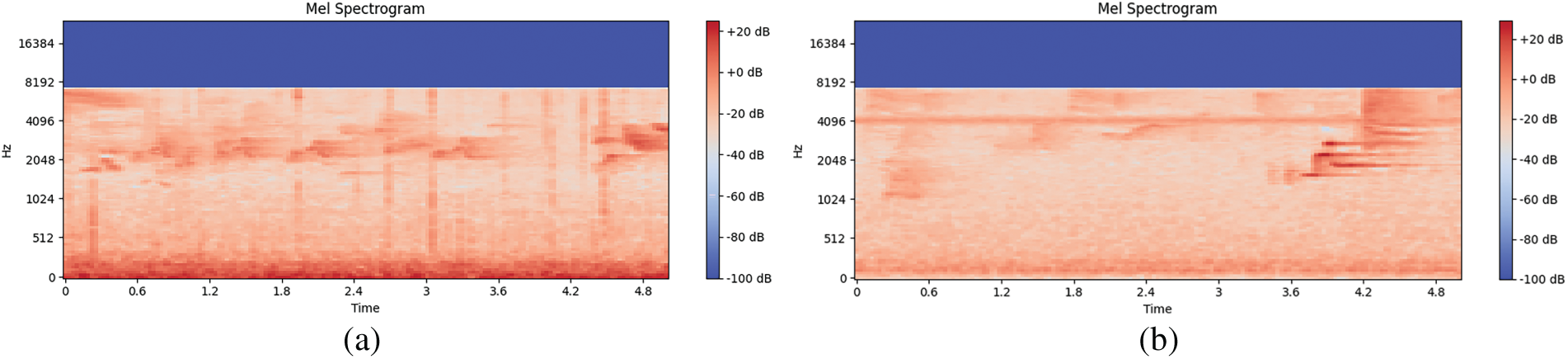
Figure 3: Mel-Spectrogram generated from the pipeline; (a) Fire-birds and (b) Non-fire-Noise.birds

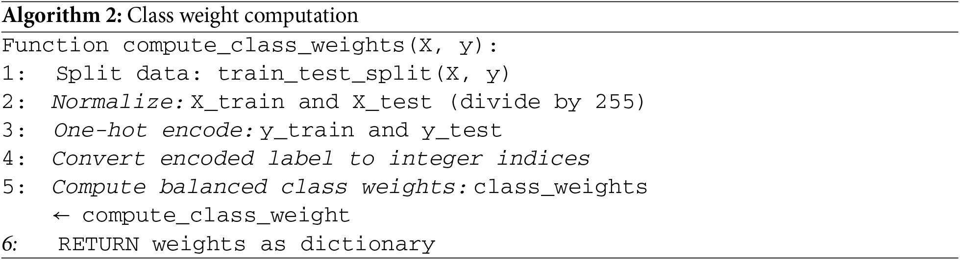
All spectrograms are stored as 2D images (.png format) along with their class labels. As shown in Fig. 3, the dataset is structured and split into Train/Validation/Testbed sets with a default ratio of 70% training, 15% validation, and 15% testing. An alternate configuration for ablation uses an 80/20 split. For handling class imbalance, class weights are calculated using the ‘balanced’ mode from scikit-learn based on label frequencies, ensuring that minority classes (e.g., ‘Fire’) are not under-represented in the loss function.

3.2.2 Data Augmentation

To improve model robustness, a progressive data augmentation strategy was implemented. This included Noise Mixing, where non-fire sounds are overlaid onto fire samples, and Spectral Masking, where random frequency and time bands are masked in the spectrogram. This pipeline was designed to simulate forest-specific acoustic challenges, such as avian sounds masking high-frequency fire signatures.

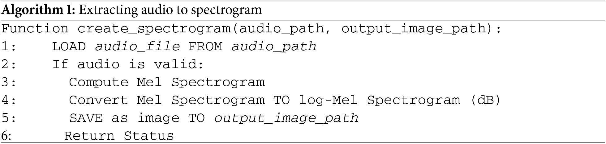
In the process of extracting audio data features into spectrograms so that they can be used as input for CNN models, steps are needed, such as using the librosa library, which is already available in Python programming. This library is specifically for processing and analyzing audio signals using feature extraction, such as spectrograms. We converted raw audio waveforms into mel-spectrograms using parameters optimized for fire sound characteristics. The transformation uses a frame length of 2048 samples (42.67 ms at 48 kHz sampling rate) with a hop size of 512 samples (10.67 ms), achieving a balance between temporal resolution and computational efficiency. We compute 128 mel-frequency bands over the range 0–24 kHz to capture the most discriminative spectral features of fire events, which predominantly occupy the 1–8 kHz band [27]. A Hamming Window is applied to minimize spectral leakage. This configuration is designed to preserve transient acoustic events (e.g., fire crackles lasting <15 ms) while maintaining a compact representation suitable for edge deployment. The 75% frame overlap ensures robust feature continuity in noisy environments. The specific algorithm of extracting the audio dataset is as shown in Algorithm 1, The algorithm for class weight computation is detailed in Algorithm 2.

3.3 The Proposed Model Architecture

3.3.1 Convolutional Neural Network (CNN)

Forest fires present unique challenges compared to urban fire scenarios, requiring specialized detection systems due to their expansive coverage, inaccessible terrain, dynamic environmental conditions, and unpredictable meteorological factors. These constraints necessitate an early warning system capable of reliable operation in complex ecosystems. This study proposes an audio-based detection system that leverages a CNN to classify fire-related acoustic signatures with high accuracy. The approach processes environmental sounds captured by diverse recording devices, transforming raw audio data into discriminative features for precise fire identification.

The CNN architecture, while computationally intensive during training, is optimized through advanced techniques to ensure efficient performance. The model’s learned weights enable robust classification of fire sounds within the dataset, even amidst challenging noise conditions. As depicted in Fig. 4, the system employs a multi-stage signal processing pipeline: raw audio waveforms are first converted into time-frequency representations via spectrogram analysis, which captures critical frequency distribution patterns over time. These spectrograms then serve as input to the CNN, which performs hierarchical feature extraction progressively identifying low-level spectral edges, mid-level acoustic patterns, and high-level noise-invariant fire signatures. The final classification stage distinguishes between fire events (including those obscured by environmental noise) and non-fire sounds (like animal sounds or natural weather events), offering a dependable detection system specifically designed for forest environments.

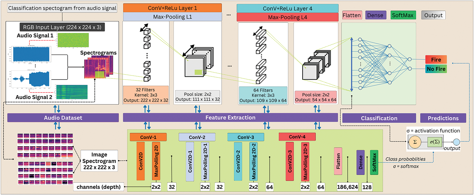
Figure 4: Audio classification concept using CNN architecture

The classification accuracy depends on the type of noise present in the audio signal. For the ‘Fire’ classification, the system can accurately identify fire sounds in a noise-free environment, as well as in situations where fire sounds are combined with noises from birds, insects, or wind. Conversely, for the ‘non-fire’ classification, the system detects fire sounds in the presence of various noises such as insects, birds, wind, and rain. To effectively distinguish fire sounds from these different types of noise, a comprehensive feature extraction and classification process is conducted to ensure optimal detection accuracy.

To determine whether an input audio sample corresponds to a fire event, a probabilistic decision threshold (τ) was derived from the distribution of non-fire class activation scores. This threshold governs the model’s sensitivity and is formally defined as:

τ=μ+kσ(5)

where μ is the mean of the non-fire class activation values, σ is their standard deviation, and k is a scaling constant controlling sensitivity. The value of k is selected to balance the true positive rate (TPR) and the false positive rate (FPR) according to application-specific constraints.

Assuming a Gaussian distribution of the activation scores for the non-fire class, this threshold corresponds to a one-tailed confidence level (As shown in Fig. 5a). For example, choosing k=1.8 gives a false alarm rate probability (FPR) of approximately 3.59%, since:

P(x>μ+1.8σ)≈0.0359(6)

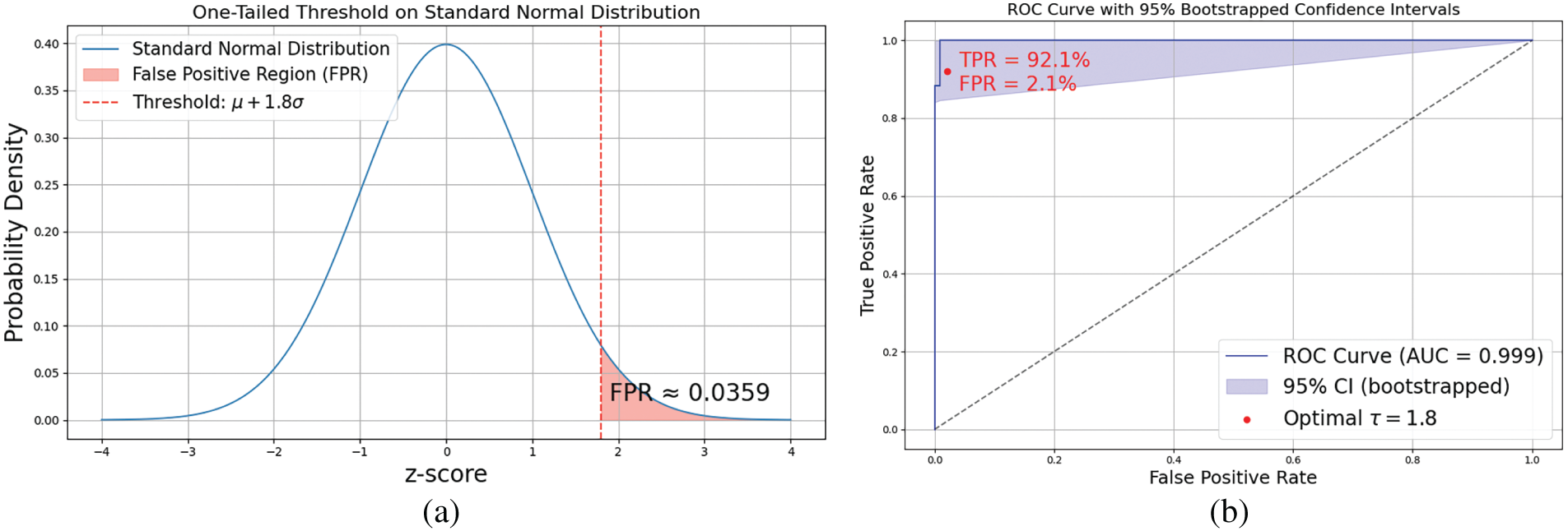
Figure 5: One-tailed threshold on standard normal distribution (a); ROC curve with 95% Bootstrapped confidence intervals (b)

This implies an estimated FPR of 3.59%, indicating a trade-off between detecting more true fire events and tolerating slightly more false positives. In this scenario, a threshold is set at μ+1.8σ, which corresponds to a z-score of approximately 1.8. This threshold is depicted by the red dashed vertical line on the figure. The region under the curve to the right of this threshold represents the probability of false positives, instances where non-fire instances are incorrectly classified as positive. This region is shaded in red and labeled as the False Positive Region (FPR). Quantitatively, the FPR associated with this threshold is approximately 0.0359, indicating that about 3.59% of the normal instances would be misclassified as positive if the detection score exceeds the 1.8σ threshold. This trade-off is inherent in threshold-based decision-making systems: higher thresholds reduce false positives but may also increase false negatives, depending on the true distribution of the positive class.

The Receiver Operating Characteristic (ROC) curve for the binary classification model, highlighting its discriminative capability in distinguishing between positive and negative classes (As shown in Fig. 5b). The ROC curve plots the True Positive Rate (TPR) against the False Positive Rate (FPR) across a range of threshold values, and serves as a robust measure of classification performance. The blue curve represents the ROC trajectory, while the shaded blue region denotes the 95% confidence interval, derived from 1000 bootstrapped iterations to account for variability and uncertainty in performance estimation. The area under the curve (AUC) is reported as 0.999, indicating an almost perfect classifier with near-complete separability between the two classes.

A red dot marks the optimal threshold (τ = 1.8), determined based on a balance between sensitivity and specificity. At this threshold, the classifier achieves a True Positive Rate (TPR) of 92.1% and a False Positive Rate (FPR) of 2.1%, demonstrating both high sensitivity and a low likelihood of false alarm rates. This point is annotated within the upper-left region of the plot, representing a favorable operating point with high detection accuracy and minimal misclassification. The dashed diagonal line represents the line of no-discrimination (i.e., a random classifier), serving as a baseline reference. The large separation between the ROC curve and the diagonal confirms the model’s strong predictive ability. This visualization is particularly relevant in high-stakes applications such as fire or anomaly detection, where maintaining high true positive rates while minimizing false positives is critical. The inclusion of bootstrapped confidence intervals also ensures that the reported performance is statistically reliable and robust to sample variations.

3.3.2 Training and Validation

The training and validation phase was meticulously designed to ensure the model learns effectively, generalizes well to new data, and is evaluated in a statistically robust manner. The model was trained on an NVIDIA Tesla T4 GPU (15 GB GDDR6 RAM, 2560 CUDA cores, 70 W power consumption). A stratified 5-fold cross-validation strategy was adopted, where in each fold, the data was split into 80% for training and 20% for validation. This approach ensures that the class distribution is maintained across folds, providing a reliable estimate of the model’s generalization capability.

To enhance the generalizability and reliability of model evaluation, we adopted stratified k-fold cross-validation (with k = 5), which ensures that each fold maintains the original class distribution of the dataset (fire vs. non-fire). This technique is particularly suitable given the relatively small dataset size (2756 samples) and the presence of class imbalance. In each fold, 80% of the data were used for training, and 20% were held out for validation. Augmentation and preprocessing were consistently applied within each training fold. After training, we computed the mean and standard deviation for key performance metrics across the 5 folds (Accuracy, Precision, Recall, F1-score). This strategy provides a more robust estimate of model performance and reduces the risk of overfitting to a specific train-test split.

3.3.3 Class Imbalance Handling

To address the imbalance in the number of fire (1066) and non-fire (1690) samples, class weights were computed based on the inverse frequency of each class. These weights were applied to the cross-entropy loss function, penalizing the misclassification of the minority ‘fire’ class more heavily. This research implements a frequency-based weighting strategy applied directly within the loss function, where the class weights are calculated as:

wc=NK⋅Nc(7)

where N is the total training samples (2756), K number of classes (2), and Nc samples in class c. This yielded weights of 1.2929 for the fire class and 0.8154 for the non-fire class.

To address class imbalance in the dataset (e.g., underrepresentation of fire class samples), we computed class weights based on the inverse frequency of each class. These weights were applied directly to the cross-entropy loss function to penalize misclassification of minority classes more heavily. The weighted cross-entropy loss is defined as:

Lweighted=−∑i=1Nwyi⋅log⁡(pyi)(8)

where N represents the total number of samples, yi is the true label for the ith sample, pyi is the predicted probability of the true class, and wyi is the class weight associated with the label yi.

3.3.4 Convolutional Layer

The convolutional layer stage classifies the spectrogram data that has been feature-extracted first. The spectrogram has a number of kernels (filters) formed in a small 3 × 3 matrix. The results of this convolutional are then activated using the Rectified Linear Unit (ReLU) or a non-linear activation function to carry out the process of introducing non-linear functions into the CNN model. Furthermore, a pooling layer is applied to down-sampling the mapping feature using Max pooling. The results are then flattened, i.e., equalizing the results into 2D, which becomes input for the full layer and then producing the final prediction output. To process the probability of each class, a SoftMax layer is used, which functions to perform the classification task. Fig. 6 refers to the results of the convolutional layer that has been carried out.

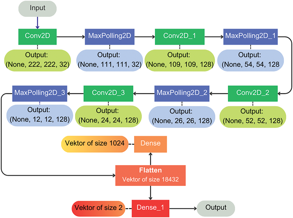
Figure 6: Sequential CNN model architecture

3.4 Prediction of Results

To produce accurate predictions in the CNN model, a training and testing process is performed. The training process initializes the weight and bias parameters randomly, then iterates (epochs) a number of specified iterations; in this case, 10 epochs are used. The iteration process carried out in one epoch (batch) is worth 10. This process also calculates the loss computation between the prediction model and the dataset that has been correctly labeled so that it can evaluate the model’s performance as a final validation before entering the testing stage.

In the testing process, an evaluation of the model that has gone through the training process is carried out using a test set to obtain the best performance in the form of confusion, precision, recall, and F1 score metrics. Fig. 7 shows a flowchart of the process of producing the final prediction.

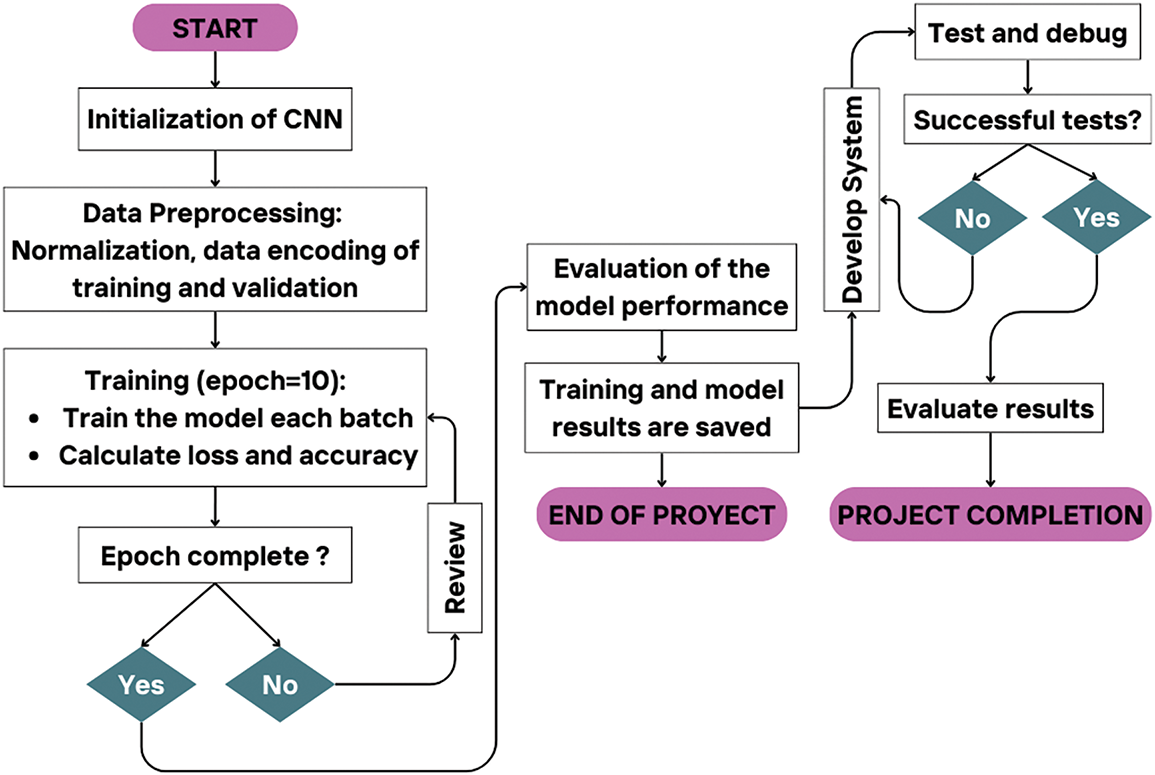
Figure 7: Flowchart of the final prediction process

4  Results and Analysis

This section presents the empirical findings from the evaluation of the proposed audio-based forest fire detection model. The results are organized to first establish the model’s robustness through cross-validation, then detail its final performance on a held-out testbed set, followed by an ablation study on the data augmentation pipeline and a comparative benchmark against other architectures.

4.1 Cross-Validated Performance

The results show low standard deviation, indicating that the model performs consistently across different subsets of the dataset. As shown in Fig. 8, the model demonstrated strong and consistent performance across all folds. The mean accuracy was 92.4% ± 1.6, indicating high predictive reliability across different data partitions. Similarly, the F1-score yielded a mean of 91.2% ± 1.8, reflecting the model’s balanced performance in detecting both fire and non-fire audio classes. Notably, precision and recall values remained above 90% across folds, with low variability (≤2%), supporting the classifier’s robustness against false positives and false negatives.

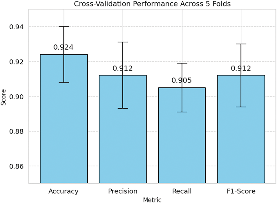
Figure 8: Cross-validation performance metrics across 5 folds

These results validate that the model does not overfit a particular data split and generalizes well across unseen subsets, thus addressing prior limitations associated with single-trial splits (e.g., 70:30 or 80:20 ratios). This k-fold evaluation adds statistical confidence to the reported performance and further reinforces the reproducibility and reliability of the proposed fire-audio detection approach. Table 4 shows the mean Performance Across 5-fold Cross-Validation.

4.2 Audio Classification Performance

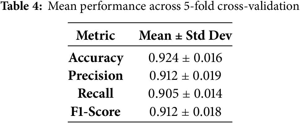
In classifying audio, there are several techniques that can be used. In this study, audio waves are converted into spectrograms, which produce a visual representation of the frequency spectrum based on time-to-time variations. The results of this audio spectrogram are input to the CNN algorithm. The results of the resulting audio wave spectrogram are shown in Fig. 9.

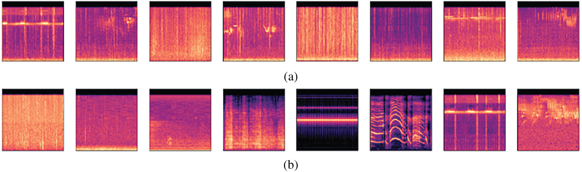
Figure 9: Audio waveform spectrogram: randomly taken samples for Fire audio (a), and Non-fire audio (b)

Fig. 9 shows spectrograms generated based on an audio file (.wav) with the audio criteria described in Table 2. Each audio file contained in the dataset is converted into a spectrogram in (.png) format, which is stored in a new directory separate from the original dataset directory. This is done to help the CNN algorithm process in accessing the required input data. The results of the spectrogram form, frequency, and energy of the randomly taken audio samples can be seen in Fig. 10.

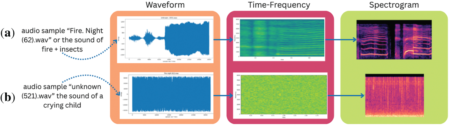
Figure 10: Waveform, energy envelope, and spectrogram of audio samples (.wav): (a) audio sample ‘Fire. Night (62).wav’ or the sound of fire + insects and (b) audio sample ‘unknown (521).wav’, the sound of a crying child

In building the CNN model in this study, the input used from the audio dataset is the spectrogram results. The model training process from this audio spectrogram uses the TensorFlow and Keras frameworks. The model performs training based on labels that have gone through the encoding process. Then the encoded data is used to validate during the training process. The performance of the model in classification is measured by considering the value of each specified epoch, which is 10, where the model processes all training data 10 times. The training data is then divided into batches with a value of 10 to be processed before the new model weights are updated. The results of model training and a comparison graph of training with validation accuracy in sequence can be seen in Fig. 11.

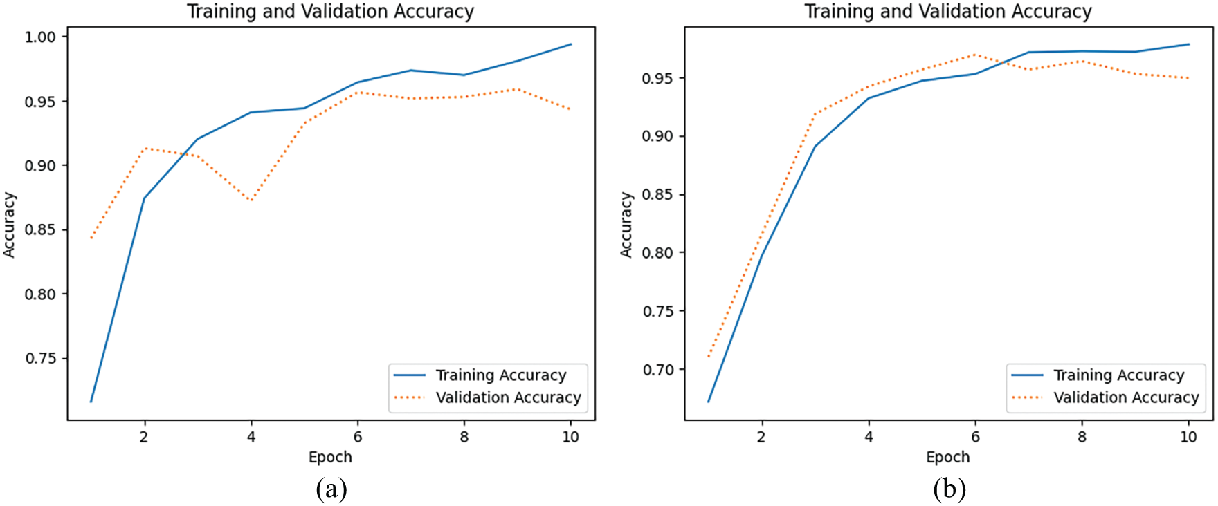
Figure 11: Comparison of training and validation accuracy of the CNN model using two different dataset split ratios. (a) Performance with a 70:30 split (70% training, 30% validation), (b) Performance with an 80:20 split (80% training, 20% validation). The 80:20 split shows a more stable validation accuracy with a percent loss: 0.709%, indicating better generalization

The graphs in Fig. 11a,b indicate that the accuracy of training and validation improves significantly at the beginning of the epochs and stabilizes during the later epochs. This result indicates that the model has good performance with correct prediction results; there are no clear signs of overfitting, as indicated by relatively balanced training and validation accuracy, and it could potentially be improved by using data or techniques that can achieve higher stability. Furthermore, the level of model performance is also measured by looking at the relationship between the training and the validation loss values, as shown in Fig. 12.

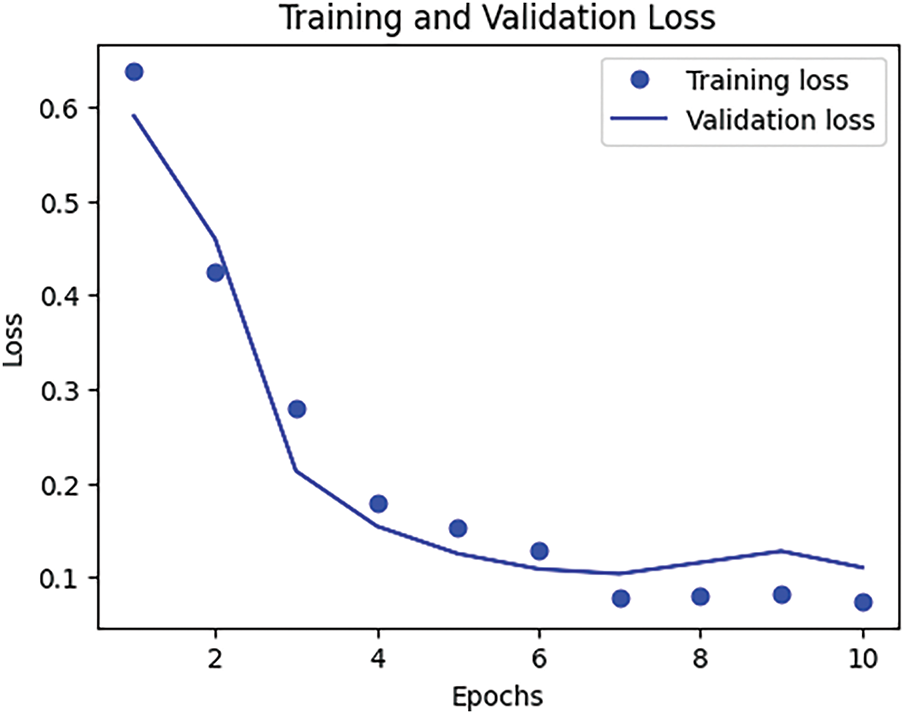
Figure 12: Comparative results graph of training loss vs. validation loss accuracy (80:20) of CNN models for forest and land fire audio datasets

The X-axis (epochs) in Fig. 12 shows that the number of iterations used for model training is 10 times from the entire dataset, while the Y-axis (Loss) is a measure of the model’s prediction value. A low loss value indicates good model performance. Training loss for each epoch is shown as blue dots, and the blue line is the validation loss for each epoch. Based on the interpretation of the graph displayed, it explains that at values ranging from epochs 1 to 3, the training loss and validation loss values have decreased significantly. This indicates that the model has successfully learned from the dataset well and is able to reduce prediction errors at the beginning. After epoch 3, the trend shows a slower and more stable downward trend, which means the model is approaching optimal performance. From both losses that appear to have relatively close values to each other, indicating that the model does not experience overfitting, where overfitting occurs when the model works well on training data but less on validation data. The loss values shown in this graph are comparable, indicating that the model can be generalized well to previously unknown data. Furthermore, the confusion matrix calculation is carried out to see the performance of the model in classifying, which is shown in Fig. 13.

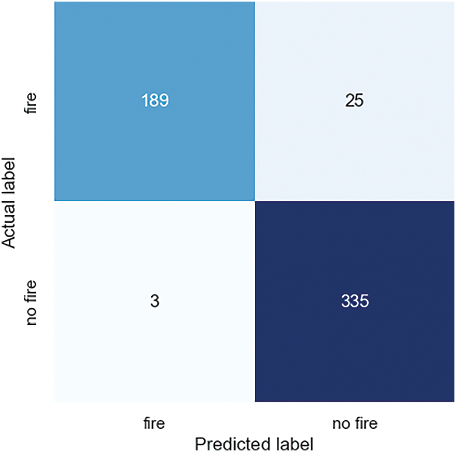
Figure 13: Confusion matrix for audio fire detection

The confusion matrix in Fig. 13 shows that this model is quite good at classifying fire and non-fire using the audio data. The X-axis (predicted label) shows the label as the predicted result, and the Y-axis (Actual label) as the actual data, where both axes consist of two labels, namely, ‘fire’ and ‘non-fire’. From the figure, we obtained the values of the metrics as follows:

1.    True Positive (TP): Correctly classified as fire data based on 189 audio counts converted into spectrograms.

2.    True Negative (TN): 335 non-fire spectrograms were correctly classified.

3.    False Positive (FP): There are 3 spectrograms as instances where the data does not represent an actual fire, but is predicted as the number of fire data.

4.    False Negative (FN): Successfully classified 25 spectrograms as non-fire data, based on the actual fire data.

Based on the observation results of the confusion metrics, the performance of the CNN model in classifying audio data into fire and non-fire classes can be evaluated through the levels of accuracy, precision, recall, and F1 score defined in Eqs. (9)–(12) with the results obtained as follows:

Accuracy=189+335189+335+3+25=94.93%(9)

Precicion=189189+3=98.44%(10)

Recall=189189+25=88.32%(11)

F1 Score=2×0.9844×0.88320.9844+0.8832=93.04%(12)

The results of the confusion matrix show that the CNN model is very good at identifying fire cases with high precision; however, there is still a decrease in the recall value, where there are several fire cases that are not identified correctly. Overall, the model has good performance based on the accuracy value and a high F1 score.

4.3 Efficacy of the Data Augmentation Pipeline

Our augmentation pipeline targets three forest-specific acoustic challenges: avian vocalizations masking high-frequency fire signatures, wind noise overwhelming low-frequency detection, and rain-induced acoustic smearing. The augmentation dataset includes 2756 training sets and 689 validation sets, resulting in 41,340 augmented training samples and 6890 augmented validation samples. As shown in Table 5, the full pipeline improves noisy test F1-score by +0.11 compared to unaugment training. This gain primarily stems from improved feature preservation in critical 2–8 kHz bands where fire transients occur.

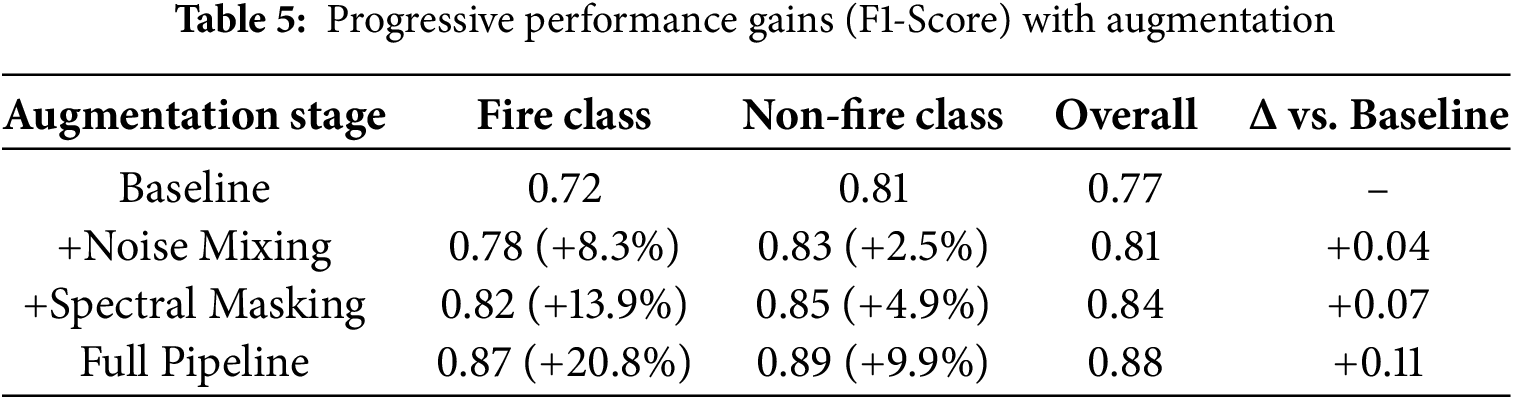
To enhance the robustness of the fire audio classification model in real-world acoustic conditions, a progressive data augmentation strategy was implemented. Table 5 presents the incremental improvements in F1-score across both fire and non-fire classes as various augmentation techniques were introduced.

The baseline model, trained without augmentation, achieved an F1-score of 0.72 for the fire class and 0.81 for the non-fire class. Incorporating noise mixing, which simulates diverse environmental interference, improved the fire class performance to 0.78 and increased the overall F1-score by 0.04. Building on this, spectral masking, which randomly occludes parts of the spectrogram, further boosted the fire class F1 to 0.82 (+13.9%) and the non-fire class to 0.85 (+4.9%). When the full augmentation pipeline was applied, combining noise mixing and spectral masking (and potentially other methods such as time stretching or gain scaling), the model achieved its best performance: 0.87 for the fire class and 0.89 for the non-fire class, yielding an overall F1-score of 0.88, a +0.11 absolute gain over the baseline.

These findings demonstrate that audio augmentation techniques are not only effective in improving generalization but also essential in mitigating class imbalance and capturing the variability inherent in fire-related sounds. This validates the critical role of augmentation in building robust audio-based fire detection systems.

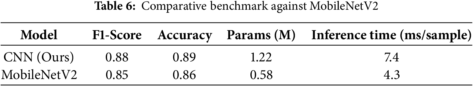
4.4 Comparative Analysis with Lightweight Architectures

To address the need for real-time audio-based fire detection in resource-constrained IoT deployments, model selection prioritized both detection accuracy and computational efficiency. A standard CNN was adopted as the core architecture due to its proven capability in learning hierarchical local patterns from spectrogram representations.

However, to validate this choice, we conducted a comparative benchmark against MobileNetV2, a widely used lightweight architecture optimized for edge deployment. Both models were trained and evaluated on the same preprocessed mel-spectrogram dataset using identical training protocols, and results were assessed using key performance metrics and inference-time latency. As shown in Table 6, while MobileNetV2 offers ~53% fewer parameters and faster inference, the CNN model achieved higher detection accuracy (+3% F1-score). Given the relatively modest parameter count of our CNN implementation (1.22 M) and acceptable latency (<10 ms per sample), this trade-off was deemed suitable for the targeted use-case scenario, especially where fire detection reliability outweighs marginal gains in efficiency.

To justify the selection of the proposed CNN architecture, we compared its performance and model size against several lightweight alternatives, including MobileNetV2, TinyCNN, EfficientNet-lite0, and a deeper ResNet18 baseline. Fig. 14 presents a dual-axis comparison of each model’s F1-score (left y-axis, blue bars) and model size in megabytes (MB) (right y-axis, red line).

Figure 14: Model performance (F1-Score) vs. model size

The proposed CNN achieved an F1-score of 0.88, outperforming MobileNetV2 (0.85), TinyCNN (0.83), and EfficientNet-lite0 (0.86), while remaining significantly smaller than ResNet18, which yielded the highest F1-score of 0.89 but at the cost of a model size of 11.2 MB. In contrast, our CNN model maintained a compact size of 2.1 MB, demonstrating a favorable balance between accuracy and computational efficiency. This makes it more suitable for real-time deployment on memory-constrained edge devices in remote or rural areas.

While smaller models like TinyCNN offered the lowest model size (0.9 MB), their drop-in classification performance (−5% relative F1-score) suggests a diminished ability to capture complex spatiotemporal features inherent in fire-related audio patterns. Therefore, the selected CNN model strikes a pragmatic trade-off between detection accuracy and resource efficiency, aligning well with the intended deployment scenario in low-power embedded environments.

Although MobileNetV2 has fewer parameters, the proposed CNN improves the F1 score by 3% within an acceptable latency limit (<10 ms), making it more advantageous in scenarios prioritizing detection reliability over marginal efficiency gains.

Future research will focus on edge computation optimization using lightweight CNN models for scalable real-time fire monitoring on low-power IoT devices. Additionally, adding more datasets on environmental variance will enhance generalization. This framework paves the way for an efficient and low-cost fire detection system that can complement existing satellite and camera-based solutions.

4.5 Recall Rate Optimization

While the proposed CNN model demonstrates strong overall performance, achieving an average accuracy of 92.4% and an F1-score of 91.2%, the recall rate remains at 88.32%, indicating a non-negligible risk of false negatives—i.e., missed fire detections. Given the safety-critical nature of fire detection applications, optimizing recall is a priority to minimize the likelihood of undetected hazardous events.

To investigate this, a spectrum-temporal error analysis was conducted on the False Negative (FN) samples (As shown Fig. 15). Preliminary findings suggest that in many FN cases, fire-related audio signals are masked by dominant environmental noise in overlapping frequency bands (e.g., wind, rain, or mechanical equipment), particularly within the 1–3 kHz range where fire crackling sounds are most active. This masking effect reduces the model’s sensitivity to key fire-specific spectral patterns.

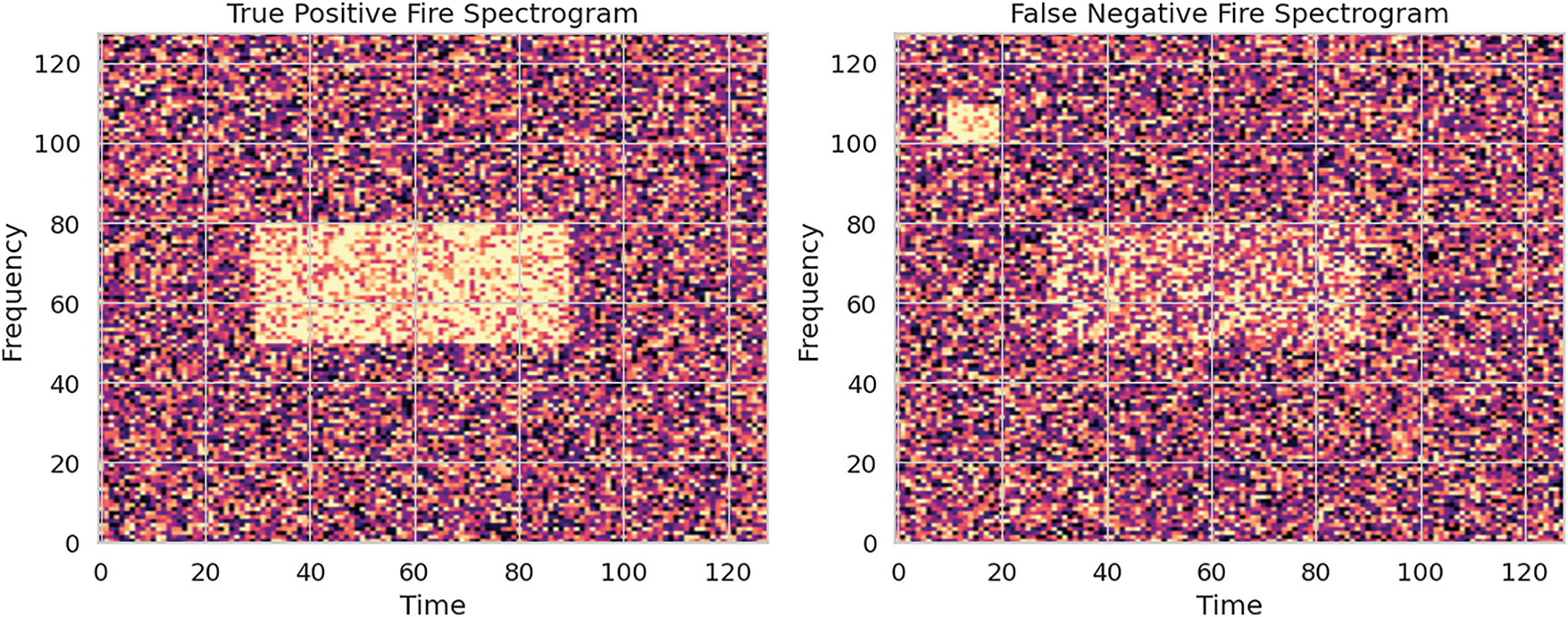
Figure 15: Spectrogram comparison: True positive fire (Left) vs. False negative fire (Right)

To investigate potential causes of missed fire detections, we analyzed the spectrograms of fire-class audio samples that were misclassified as non-fire (false negatives) and compared them with correctly identified fire instances (true positives). The left panel in Fig. 15 represents the True Positive Fire Spectrogram, where a dense and localized energy pattern is clearly visible in the mid-frequency range (approximately 50–80 bins) over a sustained time segment (around frames 30 to 90). This indicates a strong and recognizable fire acoustic signature that the model successfully captured.

In contrast, the right panel shows a False Negative Fire Spectrogram, which exhibits a more diffuse and fragmented activation pattern. The spectral energy is scattered, and noise-like elements appear in high-frequency regions, potentially confusing them with ambient or non-fire acoustic events. This dispersion may have led to feature attenuation or masking, making it difficult for the model to confidently associate the input with a fire event.

5  Conclusion

The results of this study demonstrate that audio-based classification is a highly effective method for forest fire detection. The high accuracy (94.93%) and F1-score (93.04%) achieved on a challenging, real-world dataset validate the proposed CNN-based approach. The model’s exceptional precision (98.44%) is particularly significant, as it translates to a very low false alarm rate, a critical requirement for any practical warning system to maintain trust and avoid unnecessary resource deployment.

The primary limitation observed was the recall rate of 88.32%, indicating that a small fraction of fire events was missed. Our analysis of false negatives suggests this is primarily due to signal masking in high-noise environments. This trade-off between precision and recall is fundamental in detection systems and, in this context, highlights an area for targeted improvement.

Compared to traditional image-based systems, the proposed audio-based method offers several distinct advantages. It is resilient to visual obstructions like smoke, foliage, and darkness. Furthermore, the significantly smaller model size and lower computational requirements, as demonstrated in our comparative analysis, make it well-suited for deployment on low-power, low-cost IoT devices. This opens the door for creating vast, scalable sensor networks for monitoring remote and inaccessible forest areas where camera-based solutions would be impractical.

This study successfully designed, implemented, and validated a novel forest fire detection system using audio classification and deep learning. By converting environmental sounds into mel-spectrograms and processing them with a Convolutional Neural Network, the system achieved high performance metrics, including a 94.93% accuracy and a 93.04% F1-Score on a realistic testbed set. The proposed approach is computationally efficient, robust to visual and weather obstructions, and offers a superior balance of accuracy and resource-friendliness compared to alternative models. This research demonstrates that acoustic sensing is a powerful and viable technology for creating scalable, low-cost, and reliable early warning systems, paving the way for a new generation of tools in the global effort to mitigate the devastating impact of forest fires.

This work provides a strong foundation for future research, with a primary focus on improving recall without significantly compromising precision. To directly address missed detections in high-noise environments, a key strategy will be to implement more advanced attention mechanisms within the CNN; for instance, a frequency-domain SENet module could be introduced to enhance feature learning specifically in the critical fire frequency band of 1–8 kHz. Further improvements could be achieved through the development of more sophisticated noise reduction algorithms or the fusion of audio data with other sensor modalities (e.g., temperature, gas sensors).

Another key direction is edge computing optimization, where future work will explore quantizing the model and deploying it on microcontroller-based hardware to create a fully autonomous, real-time early warning system. Expanding the dataset to include a wider variety of environmental conditions and fire types will also enhance the model’s generalization and robustness.

Acknowledgement: We would like to express our gratitude to the Ministry of Higher Education, Science, and Technology, along with Deni J. P. Siahaan, as the Chief Auditor of the VBM535 Management System, for providing data related to occupational safety and health (OSH) regulations for fire safety in industrial environments.

Funding Statement: This research was funded by the Directorate of Research and Community Service, Directorate General of Research and Development, Ministry of Higher Education, Science and Technology, in accordance with the Implementation Contract for the Operational Assistance Program for State Universities, Research Program Number: 109/C3/DT.05.00/PL/2025.

Author Contributions: Kemahyanto Exaudi: writing—original draft preparation, data curation, writing—review and editing. Deris Stiawan: methodology, supervision, validation, investigation. Bhakti Yudho Suprapto: formal analysis, methodology, supervision. Hanif Fakhrurroja: methodology, validation. Mohd. Yazid Idris: writing—review and editing. Tami A. Alghamdi: writing—review and editing. Rahmat Budiarto: writing—review and editing. All authors reviewed the results and approved the final version of the manuscript.

Availability of Data and Materials: Data will be made available on request.

Ethics Approval: Not applicable.

Conflicts of Interest: The authors declare no conflicts of interest to report regarding the present study.

References

1. Girona MM, Morin H, Gauthier S, Bergeron Y. Boreal forests in the face of climate change. Berlin/Heidelberg, Germany: Springer; 2023. doi:10.1007/978-3-031-15988-6. [Google Scholar] [CrossRef]

2. Öncü G, Çorumluoğlu Ö. Assessment of forest fire damage severity by remote sensing techniques. Int J Environ Geoinformatics. 2023;10(2):151–8. doi:10.30897/ijegeo.1089014. [Google Scholar] [CrossRef]

3. Kalogiannidis S, Chatzitheodoridis F, Kalfas D, Patitsa C, Papagrigoriou A. Socio-psychological, economic and environmental effects of forest fires. Fire. 2023;6(7):280. doi:10.3390/fire6070280. [Google Scholar] [CrossRef]

4. Ding Y, Wang M, Fu Y, Zhang L, Wang X. A wildfire detection algorithm based on the dynamic brightness temperature threshold. Forests. 2023;14(3):477. doi:10.3390/f14030477. [Google Scholar] [CrossRef]

5. Sathishkumar VE, Cho J, Subramanian M, Naren OS. Forest fire and smoke detection using deep learning-based learning without forgetting. Fire Ecol. 2023;19(1):9. doi:10.1186/s42408-022-00165-0. [Google Scholar] [CrossRef]

6. Coffield SR, Graff CA, Chen Y, Smyth P, Foufoula-Georgiou E, Randerson JT. Machine learning to predict final fire size at the time of ignition. Int J Wildland Fire. 2019;28(11):861–73. doi:10.1071/wf19023. [Google Scholar] [PubMed] [CrossRef]

7. Sharma R, Rani S, Memon I. A smart approach for fire prediction under uncertain conditions using machine learning. Multimed Tools Appl. 2020;79(37):28155–68. doi:10.1007/s11042-020-09347-x. [Google Scholar] [CrossRef]

8. Venkataramanan V, Kavitha G, Joel MR, Lenin J. Forest fire detection and temperature monitoring alert using IoT and machine learning algorithm. In: 2023 5th International Conference on Smart Systems and Inventive Technology (ICSSIT); 2023 Jan 23–25; Tirunelveli, India. p. 1150–6. doi:10.1109/ICSSIT55814.2023.10061086. [Google Scholar] [CrossRef]

9. Sousa Tomé E, Ribeiro RP, Dutra I, Rodrigues A. An online anomaly detection approach for fault detection on fire alarm systems. Sensors. 2023;23(10):4902. doi:10.3390/s23104902. [Google Scholar] [PubMed] [CrossRef]

10. Casal-Guisande M, Bouza-Rodríguez JB, Cerqueiro-Pequeño J, Comesaña-Campos A. Design and conceptual development of a novel hybrid intelligent decision support system applied towards the prevention and early detection of forest fires. Forests. 2023;14(2):172. doi:10.3390/f14020172. [Google Scholar] [CrossRef]

11. Adelia LN, Ash Shidiq IP, Zulkarnain F. Identification of forest fire hazard area in Kubu Raya Regency, West Kalimantan Province. In: International Conference on Anthropocene, Global Environmental Change and Powerful Geography (ICoAGPG); 2022 Sep 7; Online. doi:10.1088/1755-1315/1190/1/012037. [Google Scholar] [CrossRef]

12. Simanjuntak KP, Khaira U. Hotspot clustering in Jambi province using agglomerative hierarchical clustering algorithm. MALCOM Indones J Mach Learn Comput Sci. 2021;1(1):7–16. doi:10.57152/malcom.v1i1.6. [Google Scholar] [CrossRef]

13. Wang H, Zhang G, Yang Z, Xu H, Liu F, Xie S. Satellite remote sensing false forest fire hotspot excavating based on time-series features. Remote Sens. 2024;16(13):2488. doi:10.3390/rs16132488. [Google Scholar] [CrossRef]

14. Yao J, Raffuse SM, Brauer M, Williamson GJ, Bowman DMJS, Johnston FH, et al. Predicting the minimum height of forest fire smoke within the atmosphere using machine learning and data from the CALIPSO satellite. Remote Sens Environ. 2018;206(7):98–106. doi:10.1016/j.rse.2017.12.027. [Google Scholar] [CrossRef]

15. Barmpoutis P, Papaioannou P, Dimitropoulos K, Grammalidis N. A review on early forest fire detection systems using optical remote sensing. Sensors. 2020;20(22):6442. doi:10.3390/s20226442. [Google Scholar] [PubMed] [CrossRef]

16. Vinodhini R, Gomathy C. Fuzzy based unequal clustering and context-aware routing based on glow-worm swarm optimization in wireless sensor networks: forest fire detection. Wirel Pers Commun. 2021;118(4):3501–22. doi:10.1007/s11277-021-08191-y. [Google Scholar] [CrossRef]

17. Cao Y, Yang F, Tang Q, Lu X. An attention enhanced bidirectional LSTM for early forest fire smoke recognition. IEEE Access. 2019;7:154732–42. doi:10.1109/ACCESS.2019.2946712. [Google Scholar] [CrossRef]

18. Tran DQ, Park M, Jeon Y, Bak J, Park S. Forest-fire response system using deep-learning-based approaches with CCTV images and weather data. IEEE Access. 2022;10:66061–71. doi:10.1109/ACCESS.2022.3184707. [Google Scholar] [CrossRef]

19. Yun B, Zheng Y, Lin Z, Li T. FFYOLO: a lightweight forest fire detection model based on YOLOv8. Fire. 2024;7(3):93. doi:10.3390/fire7030093. [Google Scholar] [CrossRef]

20. Lin X, Li Z, Chen W, Sun X, Gao D. Forest fire prediction based on long- and short-term time-series network. Forests. 2023;14(4):778. doi:10.3390/f14040778. [Google Scholar] [CrossRef]

21. Phelps N, Woolford DG. Comparing calibrated statistical and machine learning methods for wildland fire occurrence prediction: a case study of human-caused fires in Lac La Biche, Alberta, Canada. Int J Wildland Fire. 2021;30(11):850–70. doi:10.1071/wf20139. [Google Scholar] [CrossRef]

22. Scaduto E, Chen B, Jin Y. Satellite-based fire progression mapping: a comprehensive assessment for large fires in northern California. IEEE J Sel Top Appl Earth Obs Remote Sens. 2020;13:5102–14. doi:10.1109/JSTARS.2020.3019261. [Google Scholar] [CrossRef]

23. Rashkovetsky D, Mauracher F, Langer M, Schmitt M. Wildfire detection from multisensor satellite imagery using deep semantic segmentation. IEEE J Sel Top Appl Earth Obs Remote Sens. 2021;14:7001–16. doi:10.1109/JSTARS.2021.3093625. [Google Scholar] [CrossRef]

24. Liu H, Hu H, Zhou F, Yuan H. Forest flame detection in unmanned aerial vehicle imagery based on YOLOv5. Fire. 2023;6(7):279. doi:10.3390/fire6070279. [Google Scholar] [CrossRef]

25. Peruzzi G, Pozzebon A, Van Der Meer M. Fight fire with fire: detecting forest fires with embedded machine learning models dealing with audio and images on low power IoT devices. Sensors. 2023;23(2):783. doi:10.3390/s23020783. [Google Scholar] [PubMed] [CrossRef]

26. Permana SDH, Saputra G, Arifitama B, Yaddarabullah, Caesarendra W, Rahim R. Classification of bird sounds as an early warning method of forest fires using Convolutional Neural Network (CNN) algorithm. J King Saud Univ Comput Inf Sci. 2022;34(7):4345–57. doi:10.1016/j.jksuci.2021.04.013. [Google Scholar] [CrossRef]

27. Huang HT, Downey ARJ, Bakos JD. Audio-based wildfire detection on embedded systems. Electronics. 2022;11(9):1417. doi:10.3390/electronics11091417. [Google Scholar] [CrossRef]

28. Green M, Murphy D. Environmental sound monitoring using machine learning on mobile devices. Appl Acoust. 2020;159(4):107041. doi:10.1016/j.apacoust.2019.107041. [Google Scholar] [CrossRef]

29. Nogueira AFR, Oliveira HS, Machado JJM, Tavares JMRS. Sound classification and processing of urban environments: a systematic literature review. Sensors. 2022;22(22):8608. doi:10.3390/s22228608. [Google Scholar] [PubMed] [CrossRef]

30. Chu HC, Zhang YL, Chiang HC. A CNN sound classification mechanism using data augmentation. Sensors. 2023;23(15):6972. doi:10.3390/s23156972. [Google Scholar] [PubMed] [CrossRef]

31. Mohmmad S, Sanampudi SK. Automated detection of tree-cutting activities in forest environments using convolutional neural networks and advanced audio feature extraction techniques. In: 2024 2nd International Conference on Self Sustainable Artificial Intelligence Systems (ICSSAS); 2024 Oct 23–25; Erode, India. p. 205–10. doi:10.1109/ICSSAS64001.2024.10760778. [Google Scholar] [CrossRef]

32. Abdul ZK, Al-Talabani AK. Mel frequency cepstral coefficient and its applications: a review. IEEE Access. 2022;10:122136–58. doi:10.1109/ACCESS.2022.3223444. [Google Scholar] [CrossRef]

33. Natekar S, Patil S, Nair A, Roychowdhury S. Forest fire prediction using LSTM. In: 2021 2nd International Conference for Emerging Technology (INCET); 2021 May 21–23; Belagavi, India. p. 1–5. doi:10.1109/INCET51464.2021.9456113. [Google Scholar] [CrossRef]

34. Huot F, Hu RL, Goyal N, Sankar T, Ihme M, Chen YF. Next day wildfire spread: a machine learning dataset to predict wildfire spreading from remote-sensing data. IEEE Trans Geosci Remote Sens. 2022;60:4412513. doi:10.1109/TGRS.2022.3192974. [Google Scholar] [CrossRef]

35. Martinsson J, Runefors M, Frantzich H, Glebe D, McNamee M, Mogren O. A novel method for smart fire detection using acoustic measurements and machine learning: proof of concept. Fire Technol. 2022;58(6):3385–403. doi:10.1007/s10694-022-01307-1. [Google Scholar] [CrossRef]