Adaptive Path-Planning for Autonomous Robots: A UCH-Enhanced Q-Learning Approach

1  Introduction

With the rapid development of AI and control technology, mobile robots have been widely used in industrial manufacturing, logistics and sorting, etc. Intelligent control of mobile robots is evolving towards self-learning and adaptation. In recent years, autonomous mobile robots have gained significance due to their relevance to contemporary societal needs [1]. They are among the fastest-growing fields, capable of moving autonomously in various environments without external assistance [2]. The movement of intelligent mobile robots in complex environments is a key research interest [3]. Motion planning is a critical task for intelligent mobile robots, divided into path planning and trajectory planning [4]. In practical applications, path planning often serves as the initial step of trajectory planning. Its primary goal is to find the optimal path from a starting point to an endpoint in a given environment, with wide applications in driverless vehicles, logistics, and robot navigation. The environment in which a mobile robot operates is crucial for path planning. It can be static and unchanged or dynamically transforming. Path planning in dynamic environments is more practical and challenging [5].

In recent years, various path planning [6] algorithms have been applied to mobile robots, including Dijkstra’s, Bellman-Ford, A-Star, Rapidly-exploring Random Tree (RRT), Ant Colony Optimization (ACO), Particle Swarm Optimization (PSO), Genetic Algorithm (GA), Artificial Potential Field (APF), and Reinforcement Learning (RL). In [7], an improved Dijkstra algorithm is proposed for path optimization, combining the octagonal search method with the Dijkstra algorithm. In [8], a Bellman-Ford algorithm is proposed to solve the shortest path problem in a network within a fuzzy image environment. In [9], a path planning method based on geometric A-Star algorithm is proposed and applied in various scenarios. In [10], a convolutional neural network-based RRT algorithm is proposed for solving path planning problems. In [11], an improved Ant Colony Optimized Artificial Potential Field (ACO-APF) algorithm is proposed, combining the ACO algorithm with the artificial potential field method. This lattice graph-based algorithm is used for local and global path planning of unmanned underwater vehicles (UUVs) in dynamic environments. In [12], a new strategy for planning smooth paths for mobile robots is proposed, based on particle swarm algorithms with successive higher-order Bessel curves. In [13], an improved Genetic Algorithm (GA) is proposed to enhance mobile robots’ ability to solve path planning problems in complex maps. In [14], an improved sparrow search algorithm has been proposed for research on evacuation path planning. Basic path planning algorithms, while capable of solving issues like shortest path search, still face significant challenges. These include difficulties in environment modeling, adapting to complex environments, slow algorithm convergence, and a tendency to fall into local optima.

To tackle the challenges traditional algorithms face in modeling unknown environments and enhancing convergence speed, researchers have employed reinforcement learning (RL) algorithms for path planning. In [15], the G2RL approach is introduced to solve the path planning problem in large dynamic environments. In [16], the MAPPER approach is proposed, a decentralized, partially observable evolutionary reinforcement learning method for hybrid dynamic environments. In [17], deep neural networks and Markov Decision Process (MDP) are used for autonomous navigation of small UAVs. In [18], DRL-based algorithms are used alongside structured map data to train DDQN architectures, balancing navigation with mission objectives. In [19], the SAC algorithm combined with deep reinforcement learning is used to achieve dynamic obstacle avoidance for a robotic arm. In [20], algorithms based on two-depth Q-networks are proposed to develop QoS-based action selection strategies. In [21], an optimized TD3 model is proposed for energy-efficient and effective path planning for UAVs. In [22], a deep reinforcement learning strategy is proposed to enhance USV autopilot and collision avoidance capabilities by interacting with a simulation environment through DQN. In [23], a USV collision avoidance algorithm based on COLREGs is proposed, using a DDPG network and cumulative priority sampling to enhance efficiency. In [24], the MADPG method and Gumbel-Softmax strategy are used for AGV conflict prevention path planning. In [25], deep reinforcement learning methods are proposed for driverless ground vehicles to enable real-time planning in harsh environments. Although RL is effective in local path planning, it still faces challenges such as dimensional catastrophe and slow convergence speed.

Researchers have widely adopted Q-learning and its enhanced algorithms to address path planning in reinforcement learning, achieving remarkable results. In [26], DFQL algorithm combines Q-learning with artificial potential fields to effectively solve the path planning problem for unmanned underwater vehicles in partially known marine environments. In [27], the EQL algorithm provides fast convergence to the optimal path for mobile robots through innovative reward functions and selection strategies, improving path optimization, computational efficiency, and safety. However, in [28], the initialization of the Q-table is crucial to the performance of the algorithm. Hao et al., in [29], optimized the Q-table initialization using the Flower Pollination Algorithm (FPA) to improve path search efficiency. Although heuristic algorithms [30,31] provide feasible solutions for complex problems, there are non-optimal solutions and complexity analysis difficulties, which need to be further improved to enhance the algorithm efficiency and the learning speed of intelligences. In addition, Q-learning algorithm also suffers from credit allocation difficulties, falling into local optima, the curse of dimensionality, and over-optimization of the reward function [32,33]. Difficulty in credit allocation can cause time delays, making it hard to assess actions in real-time [34]. Local optima can prevent agents from finding better strategies [35]. Dimensionality issues can degrade model performance and increase computational complexity [36]. Over-optimization may lead to poor generalization in new environments or tasks. To address the above problems, researchers have proposed a variety of improved reward function mechanisms [37]. For example, John von Neumann and Oskar Morgenstern, pioneers in the field of reinforcement learning, introduced utility theory in game theory, which was later used to design more complex reward functions [38]. Some scholars have also proposed a variety of methods to improve reward function design, using hierarchical reinforcement learning and potentially model-based approaches to improve learning efficiency and generalisation [39]. Zhang et al. [40] introduced a novel reward function based on the Predator-Prey model to improve algorithm performance. Although these studies advance the reward function design, the adaptability and generalization ability of mobile robot path planning in dynamic environments still need further research and improvement [41].

In this work, an improved Q-learning algorithm with UCH mechanism and optimized Q-table initialization is proposed to enhance path planning efficiency and selection accuracy. The contributions of this paper are:

(1)   A variant is introduced that enhances performance by dynamically adjusting pheromone volatility, thus avoiding local optima.

(2)   We improve the Q-table initialization process of the Q-learning algorithm using an enhanced ACO algorithm.

(3)   A UCH reward mechanism is introduced that dynamically adjusts reward parameters, reducing exploration dilemmas and enabling more precise reward criterion assessment, thereby enhancing algorithm performance.

The subsequent sections of this document are structured as follows: Section 2 details the basics of RL, traditional Q-learning algorithms, and environmental modeling for path planning. Section 3 outlines an upgraded Ant Colony Optimization (PACO) algorithm to refine Q-table initialization, describes the UCH mechanism for tuning the reward function, and introduces the IQL algorithm along with its evaluation metrics. Fig. 1 briefly introduces the mechanism of the IQL algorithm proposed in this article. Section 4 elaborates on the simulation methodologies and experimental outcomes. Finally, Section 5 encapsulates the paper’s principal contributions.

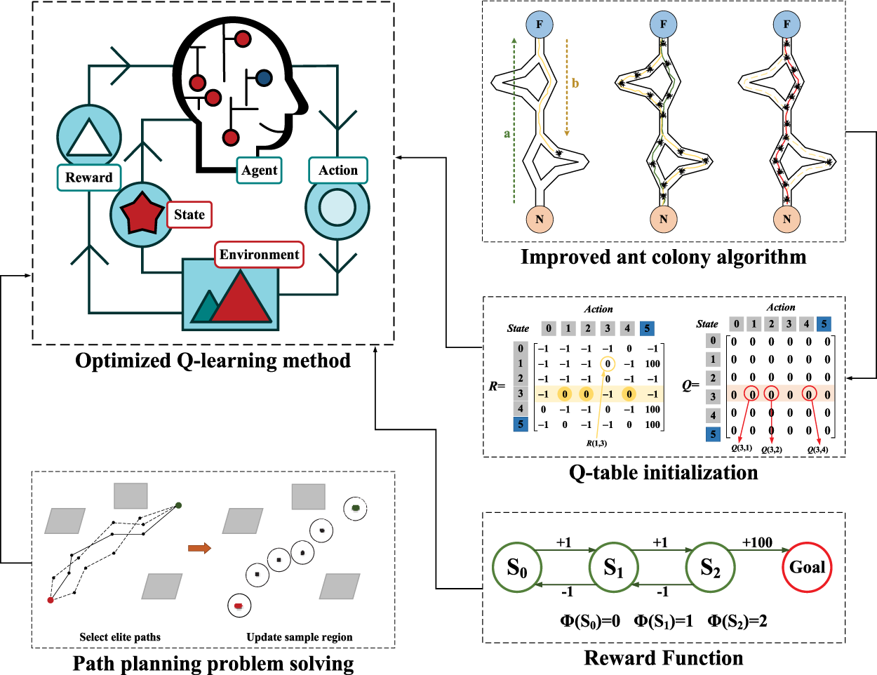
Figure 1: Framework diagram of the IQL algorithm

2  Background

This section covers the basics of RL and traditional Q-learning, focusing on reward functions and environment modeling essential for the improved Q-learning (IQL) algorithm proposed in this paper.

2.1 Reinforcement Learning

In the standard RL model, its fundamental framework is composed of three core elements: state, action, and reward. Agent [42] acquires the current state st of the environment through observation at moment t, and then performs a specific behavior a from all feasible behaviors according to an established strategy and receives a reward rt for evaluating the merit of the behavior. Subsequently, the intelligent body transfers to a new state st+1 based on the performed behavior and continues the process until the training is complete. The ultimate goal of the intelligent body is to learn a strategy S→A that results in maximizing the desired cumulative reward r. In this process, the set of states of the environment is denoted as S={s1,s2,⋅⋅⋅,st+1,⋅⋅⋅}, while all the possible behaviors constitute the set A={a1,a2,⋅⋅⋅,an}. Each behavior has a corresponding Q-value by which the intelligent body decides its behavioral choices.

2.2 Basic Q-Learning Algorithms

Q-learning algorithm [43], introduced in 1989, is a model-free reinforcement learning method that guides an agent’s actions across various states. As a classic algorithm, it doesn’t require model construction and consists of three main components [44]: Q-table initialization, action selection strategy, and Q-table update. Typically, the Q-table is initialized with constant values, and the ϵ-greedy strategy is used for action selection. The updated formula for the value function is shown in Eq. (1).

Q(s,a)=Q(s,a)+α(r(s,a)+γmaxa′Q(s′,a′)−Q(s,a))(1)

In addition to the three essential components, defining the reward function and collision handling is crucial for the path planning problem. The agent receives a penalty for each step taken, which is related to the length of the path from the previous step. When the agent hits an obstacle, it remains in place and seeks actions to avoid the obstacle until reaching the endpoint. The reward function can be defined as shown in Eq. (2).

r(s,a)=−(xs−xs′′)2+(ys−ys′′)2(2)

where s is the current agent state, and (xs,ys) is the coordinates of the current state corresponding to the raster; s′′ is the previous state of the agent, and (xs′′,ys′′) is the coordinates of the raster corresponding to the previous state.

Basic flow of Q-learning algorithm is depicted in Fig. 2.

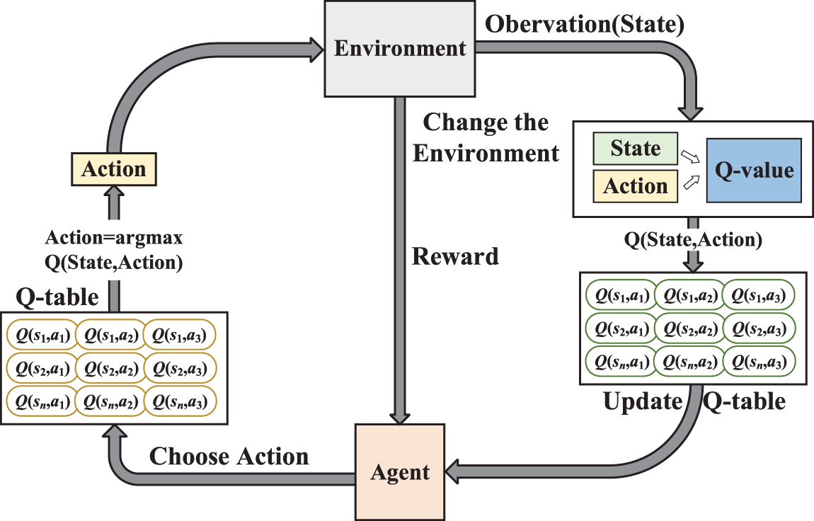
Figure 2: The interplay process between the Q-learning algorithm and the surrounding environment

Q-learning is widely used in gaming, robotics, and resource management due to its simplicity and effectiveness, providing a solid foundation for reinforcement learning. However, traditional Q-learning faces challenges such as slow iteration speed, difficulty in environment comprehension during Q-table initialization, and a tendency to fall into local optima.

2.3 Environmental Modelling for Path Planning

This paper uses the raster method to model the environment, which includes static obstacles [45]. A grid cell that contains an obstacle is marked as “1” and represented by a black grid in the simulation drawing, regardless of whether the obstacle completely covers the cell. Conversely, a grid cell that has no obstacle is marked as “0” and represented by a white grid in the simulation drawing.

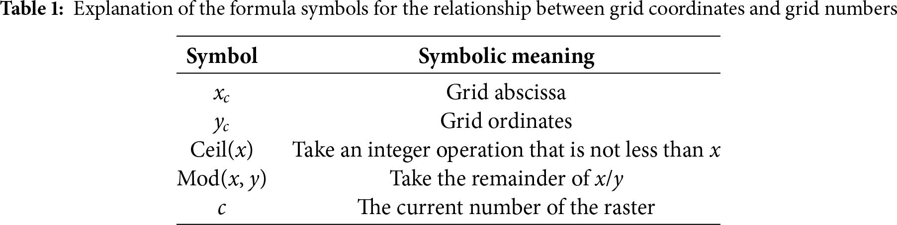
Fig. 3 is used as an example to illustrate the relationship between raster coding and horizontal and vertical coordinates [46]. Firstly, a Cartesian coordinate method is used to number grids: horizontal number of grid is used as the abscissa of grid, and vertical number of grid is used as the ordinate of grid. In Fig. 3, the maximum h of the raster abscissa is 10, the maximum v of the raster ordinate is 10, and the total number of rasters is 100. Grids are numbered 1,2,⋯,h×v from bottom to top and left to right. The relationship between the grid coordinates and the grid number is expressed as the following formula. Table 1 shows the symbols and their meanings in (3).

{xc=ceil(c/h);yc={mod(c/h),mod(c/h)≠0;h,mod(c/h)=0.(3)

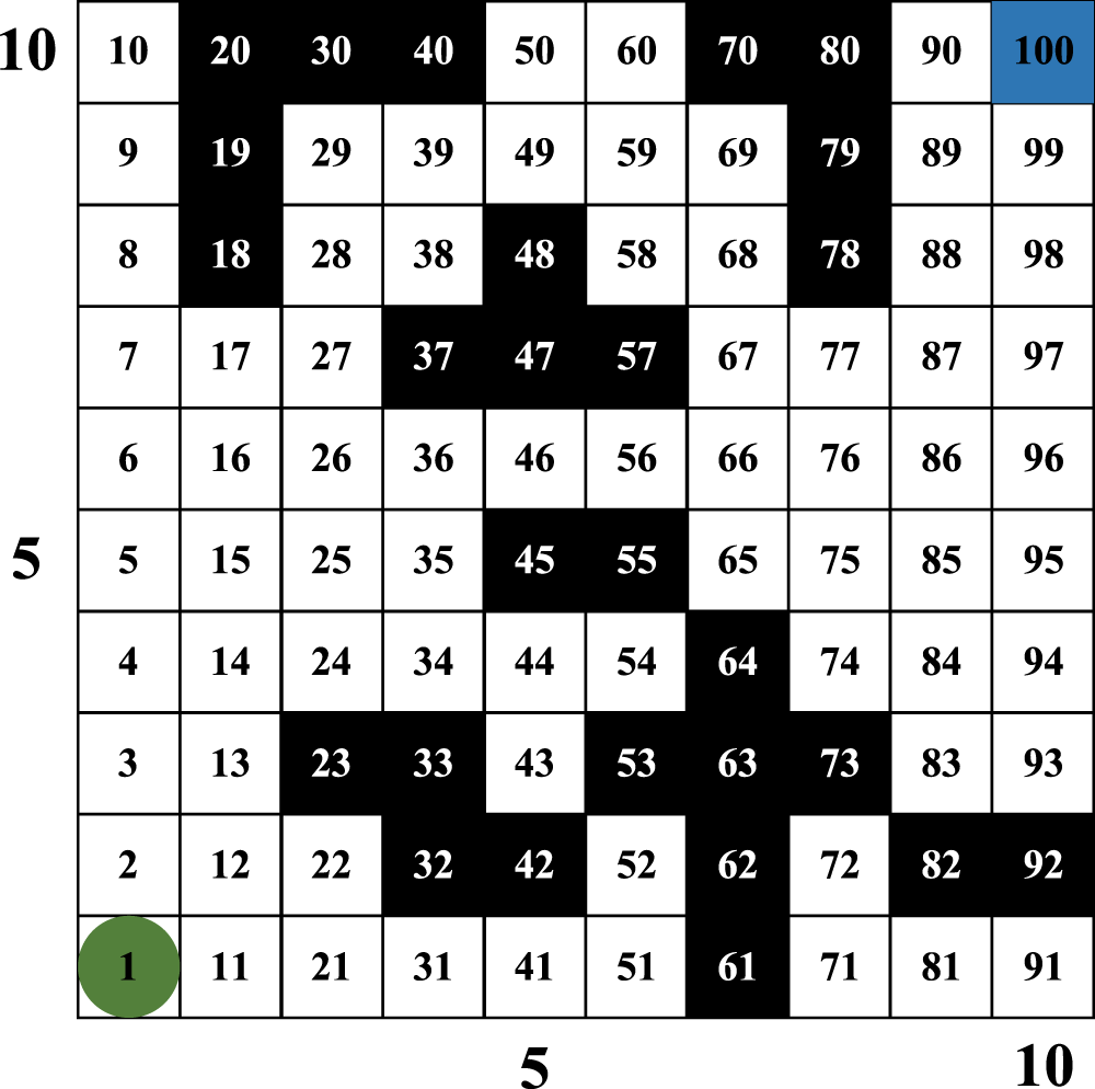
Figure 3: Raster map environment and serial number encoding

Path planning algorithm, which adopts an obstacle avoidance strategy, ensures that the planned path neither passes through obstacles nor collides with them. Fig. 4 illustrates agent’s movement from grid c to grid n, and shows the path options in 8 directions and the correct detour path.

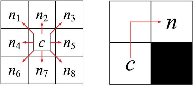
Figure 4: The selected path and the correct detour path

Fig. 5 illustrates two common error paths, which collide with obstacles and do not meet basic requirements of conditional path constraints.

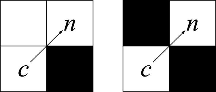
Figure 5: Two error paths

3  Methods

The IQL algorithm introduced in this paper enhances Q-learning for path planning by addressing the inefficiencies of traditional Q-tables. Leveraging the PACO algorithm for Q-table initialization, IQL enables quicker adaptation and more efficient path selection, improving both solution efficiency and accuracy. ACO was chosen over alternatives like Genetic Algorithms and Particle Swarm Optimization for its superior global optimization, adaptability to dynamic environments, and balanced exploration-exploitation. Additionally, ACO’s effectiveness in combinatorial optimization and scalability make it ideal for complex path-planning tasks.

Furthermore, the UCH mechanism was implemented to handle sparse reward functions, reducing exploration risks and enhancing the agent’s ability to identify reward criteria. These combined optimizations significantly enhance the IQL algorithm’s performance, leading to faster convergence, higher path quality, and improved obstacle avoidance, making it the preferred choice for efficient and adaptable path planning.

Overall, the IQL algorithm, which effectively adapts to the comprehensive needs of path planning efficiency, accuracy, and adaptability, accelerates convergence speed, improves path quality, and strengthens obstacle avoidance.

3.1 Q Table Initialization Optimization Strategy

(1)   PACO Algorithm

Ant colony optimization (ACO) [47] simulates the foraging behavior of real ants. During foraging, ants discharge a volatile substance called pheromones along their path, using its presence and quantity to guide their movement direction. Generally, ants tend to choose paths with more pheromones, forming a positive feedback mechanism: the pheromones on the optimal path increase, while those on other paths gradually decay over time. The ACO algorithm, which simulates this foraging action [48], is a heuristic optimization algorithm with certain advantages in solving combinatorial optimization problems. However, it also has disadvantages such as slow convergence speed, sensitive parameter settings, and a tendency to fall into local optima, which can affect the algorithm’s performance and applicability.

This paper introduces the PACO algorithm to improve ACO algorithm performance. The PACO algorithm is used as the optimization strategy for Q-table initialization, where the best solution obtained by the ACO algorithm serves as the Q-table initialization strategy.

The PACO algorithm is inspired by the feeding behavior of ants in nature and builds a distributed intelligence system. It improves the pheromone update mechanism by introducing a volatilization coefficient to prevent ants from falling into local optima, as shown in Fig. 6.

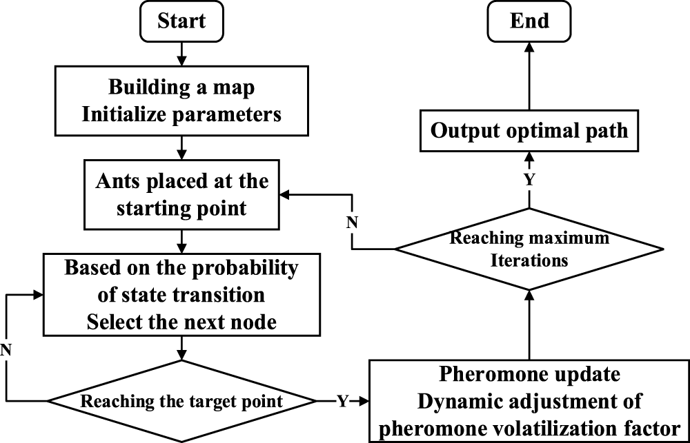
Figure 6: The PACO algorithm’s flow chart

PACO algorithm model is briefly described with the help of n random regions. Let m ants be placed on n random regions, where n is the size of the aggregation point; m denotes ants’ number; c is a set of random areas of this problem; τij(t) is the pheromone on the path region of the random region i and j at time t.

Step1: State transition guidelines.

Each ant independently selects the next region based on path pheromones and records the visited regions of ant k in the tabu table. t time t, the likelihood of ant k moving from random region i to random region j, denoted as pijk(t), is as (4).

pijk(t)={allowedk={C−tabuk}[τij(t)]αg[ηik(t)]β∑s∈allowedk[τis(t)]αg[ηis(t)]βj∈allowedk0j∉allowedk(4)

Among them, α is the information heuristic, reflecting the influence of pheromones on the path region of the ant, and β is the expectation heuristic, indicating the impact of the path area on the ant. And allowedk is the random region set that can be selected when the ant k moves next.

Step2: Pheromone updates.

In the PACO algorithm, the probability of choosing a path is proportional to the pheromone concentration on that path. Over time, pheromone levels decrease according to a defined volatility coefficient. Traditional ant colony algorithms use a fixed value for this coefficient. If set incorrectly, the colony may prematurely converge on certain paths, resulting in local optima, thereby hindering the algorithm’s ability to find the global best solution and slowing down convergence.

To address this limitation, the PACO algorithm incorporates a mechanism for dynamically adjusting the pheromone volatility factor. Instead of being a static constant, the pheromone volatility factor ρ decreases gradually with each iteration. This adjustment maintains path diversity and enhances convergence speed, as demonstrated in (5).

ρ(t)=λ1(1+eλ13m)(5)

where λ1 represents the adjustment coefficient of the pheromone volatilization factor, Nc represents the number of the current iteration, and m is the ant’s number.

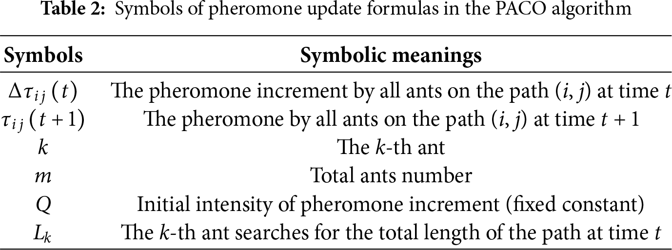
The pheromone update formula in the PACO algorithm is shown in (6).

{τij(t+1)=(1−ρ(t))⋅τij(t)+Δτij(t)Δτij(t)=∑k=1mΔτijk(t),Δτijk(t)={QLk,(i,j)∈Lk0,others(6)

Table 2 shows the symbols and their meanings in Eq. (6).

(2)   Q-Table Initialization Operation

Q-table initialization optimization strategy basis of the PACO algorithm involves these steps, which could be summarized to describe the process. Fig. 7 shows the Q-table initialization optimization strategy process based on the PACO algorithm.

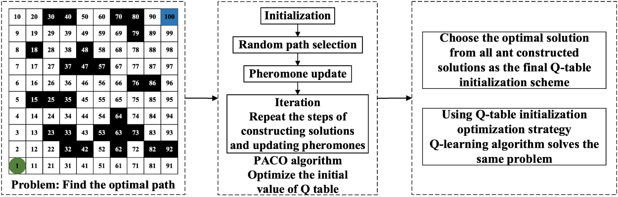
Figure 7: Initialization optimization policy process on Q-table

Step1: Problem definition.

Identify the problem of finding the optimal path that needs to be solved.

Step2: PACO algorithm parameter settings.

Set the parameters of the PACO algorithm, such as the total number of ants m, the initial intensity of pheromone increment, the expected heuristic, and the pheromone volatilization rate.

Step3: Colony initialization.

Randomly place ants at the start of the map, with each ant representing a potential solution.

Step4: Iterative path construction process.

Select the next node of the path based on the state transition probability Formula (4) and determine whether the target point is reached.

Step5: Dynamic pheromone updates.

Introducing a dynamic adjustment mechanism of pheromone volatilization factor is key. This is achieved by using the dynamic volatilization coefficient Formula (5) and pheromone update Formula (6). This ensures the diversity of paths and improves convergence speed.

Step6: Output the PACO results.

At the conclusion of the iteration, the optimal or near-optimal path P={s0,s1,⋯,sT} is selected and the τij (pheromone concentration) and path length Lk are recorded for each edge. After the algorithm is terminated, the best solution found is output as the initial value of the Q table.

Step7: Q-table initialization with PACO mapping.

The initial utility value of the ant taking different actions in each state is the IQL algorithm’s initial value. This step is a vital part of the optimization strategy. The resulting paths should be mapped to Q-learning’s (state, action) pairs, and assigned according to the following equation:

Qinit(st,at)=Qbase+β⋅τijLk(7)

In this equation, Qbase denotes the base value of the unexplored action, and β is the scaling factor.

Step8: Algorithm performance evaluation.

The enhancement in convergence speed and stability of this strategy is substantiated by a comparison of the performance discrepancy between the Q-learning method initialized with the PACO algorithm and the random initialization.

(3)   PACO-Q-Learning Integration Process

In the PACO method of IQL algorithm, the initial step is to perform path search based on state transition probability (Eq. (4)) to generate multiple candidate paths. The search quality is then continuously improved through dynamic pheromone updates (Eqs. (5) and (6)). Subsequently, the optimal path with comprehensive cost is selected from the candidate paths and mapped to (state, action) pairs. These are written into the Q-table according to the initialization formula, thereby replacing the traditional random initialization method. Subsequently, Q-learning commences from the optimised Q-table, implements the ε-greedy exploration strategy for training, and iteratively updates the Q-value using the Bellman equation (Eq. (1)) during the interaction process. This process combines PACO and Q-learning in an organic manner, thereby enhancing the convergence speed and stability of learning. As illustrated in Fig. 8, the process previously delineated is demonstrated.

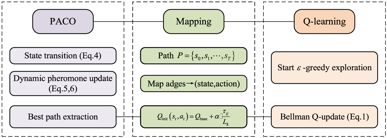
Figure 8: PACO-Q-learning integration framework

3.2 Reward Function Optimization

The reward function, a crucial component of Q-learning algorithms, determines the reward an agent receives from interacting with the environment. By optimizing the reward function, the agent can learn an effective strategy more quickly. In this section, we optimize the reward function by introducing the UCH mechanism, which significantly enhances the algorithm’s performance.

The UCH mechanism dynamically adjusts the reward parameter and changes the distance calculation method. This mechanism helps the reward function develop an effective strategy faster and in real-time. Table 3 uses Euclidean distance as an example to compare the optimized and original reward functions.

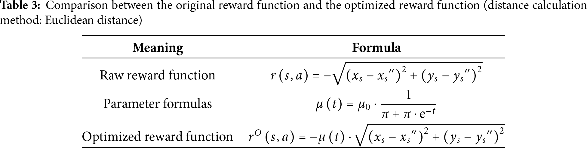
In this paper, we compare two distance calculation methods with the Euclidean distance method used in the original algorithm.

(1) Chebyshev distance

In mathematics, Chebyshev distance [49], also known as the L∞ norm, is regarded as a measure within a vector space. The distance is determined by calculating the absolute difference between two points in each coordinate dimension and taking the maximum value from these differences.

Chebyshev distance is based on the concept of a consistent norm (or supremum norm) and is classified as an injective metric space.

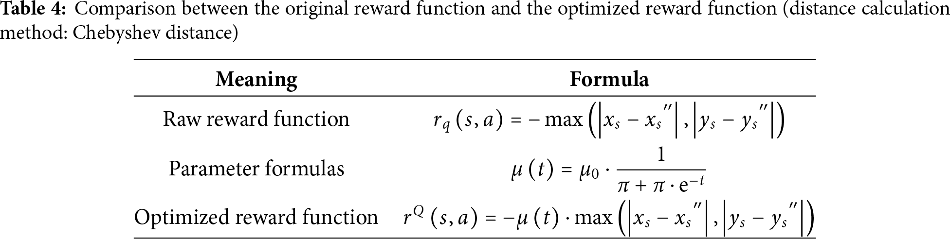
This paper focuses on the impact of distance calculation methods on algorithm performance in the two-dimensional plane and therefore considers only the Chebyshev distance. Let the Chebyshev distance between the two points on the plane be A(xs,ys) and B(xs′′,ys′′), and the Chebyshev distance of the two points AB as (8).

dABQ=max(|xs−xs"|,|ys−ys"|)(8)

Table 4 compares the optimized reward function with the original reward function using the Chebyshev distance as an example.

(2) Manhattan distance

In Manhattan neighborhoods, the driving distance from one intersection to another is not a straight-line distance between two points, and this actual distance is the “Manhattan distance [50]”. For this reason, Manhattan distance is also known as “taxi distance” or “city block distance”.

The scope of this paper is the impact of distance calculation methods on the performance of the algorithm on the two-dimensional plane, so only the Manhattan distance on the two-dimensional plane is introduced. Let the two points on the plane be A(xs,ys) and B(xs′′,ys′′) and the Manhattan distance between the two points AB as (9).

dABM=max(|xs−xs′′|,|ys−ys′′|)(9)

Fig. 9 below illustrates the difference and connection between the Euclidean distance, the Manhattan distance and the equivalent Manhattan distance.

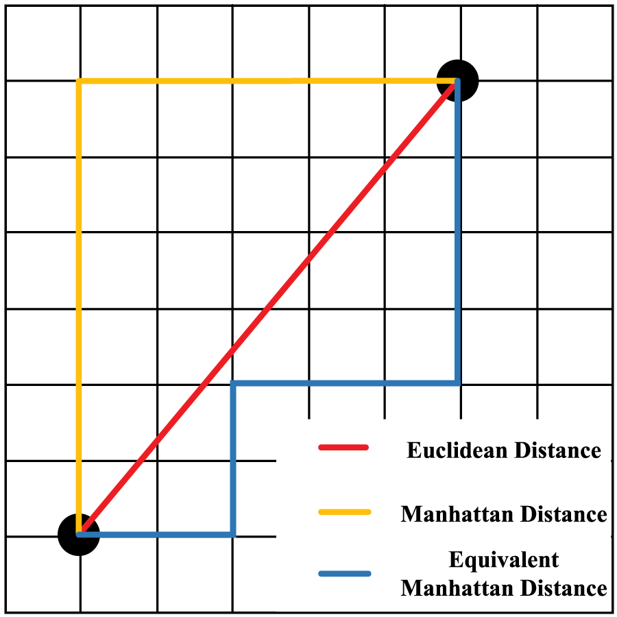
Figure 9: Euclidean distance, Manhattan distance, and equivalent Manhattan distance

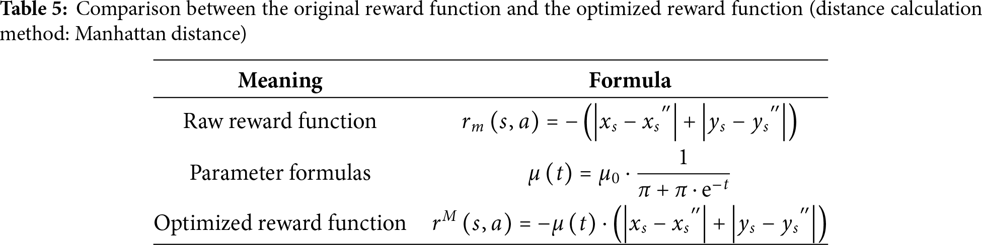
Table 5 below takes the Manhattan distance as an example to show the comparison between the optimized reward function and the original reward function.

3.3 Algorithm Pseudocode

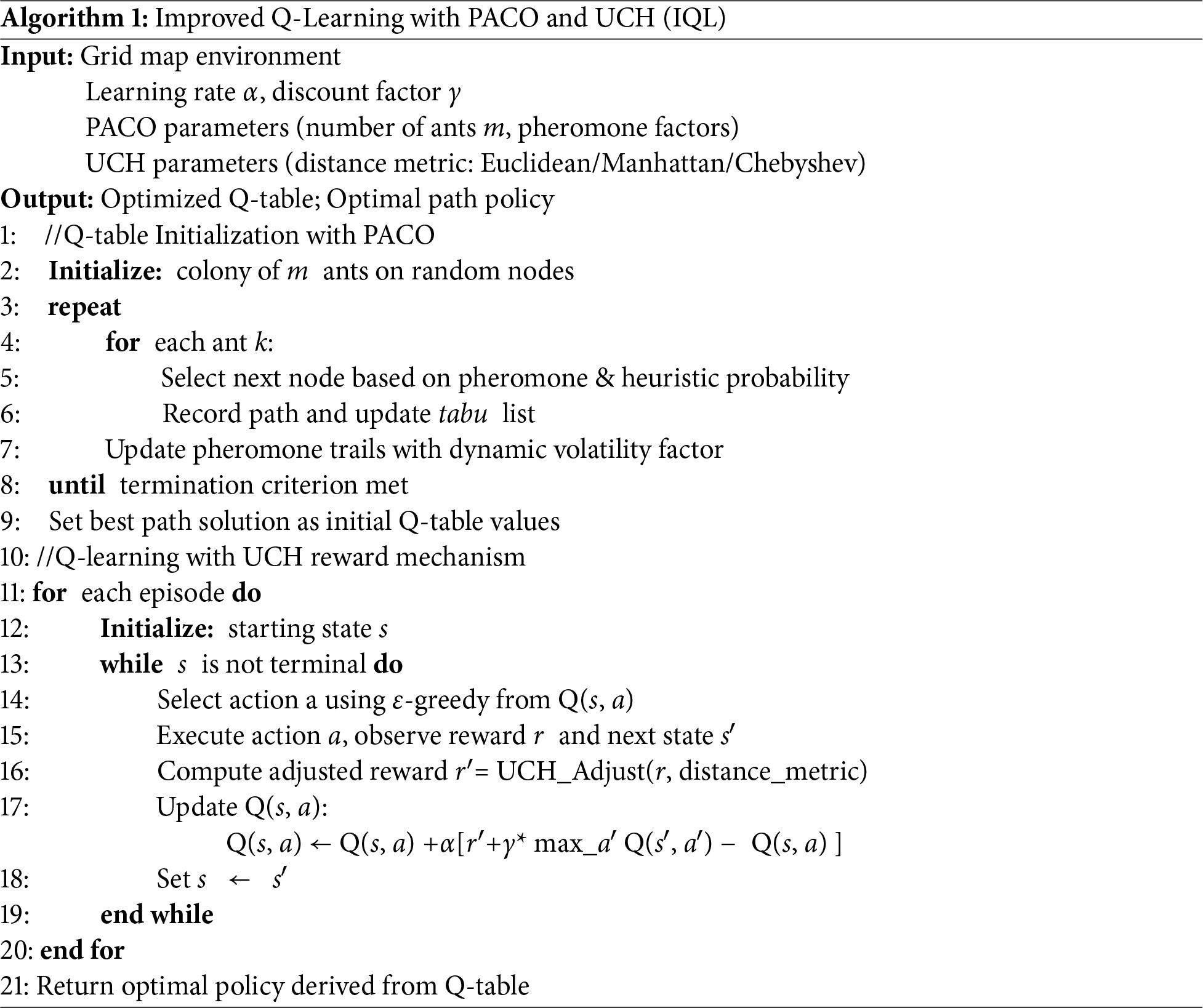
To improve the clarity of the methods we propose and enhance the readability of the paper, we provide a summary pseudocode of the improved Q-Learning (IQL) algorithm.

Although Sections 3.1 and 3.2 detail the PACO-based Q-table initialization strategy and UCH reward function optimization, respectively, the present algorithm integrates these components into a unified framework. This holistic process enables readers to quickly grasp the step-by-step execution of the IQL method. The pseudo code is shown in Algorithm 1.

3.4 Evaluation Indicators

The algorithm evaluation index is a quantitative measure of algorithm performance, encompassing learning speed, stability, and final results. These indicators provide a comprehensive evaluation of the optimized algorithm’s practical performance and form the basis for further improvement assessments.

In this study, three evaluation indicators are used to assess the improved Q-Learning (IQL) algorithms.

(1) Trials number with the same number of iterations X. With the same number of iterations, the algorithm requires fewer experiments to reach a steady state, indicating improved performance. This evaluation index η(t) reflects the learning speed and efficiency of the algorithm.

(2) The number of trials with a standard deviation of 0. The trial number required to reach a standard deviation of 0 (d(t)) is a statistic that measures the degree of dispersion in a set of numerical distributions. If the optimized algorithm achieves a standard deviation of 0 with fewer tests, it indicates improved measurement stability, reduced systematic error, and enhanced data reliability.

(3) The expected return after the algorithm’s convergence. Expected return (e(t)) refers to the average cumulative return an agent receives from the initial state when following a strategy. The agent can better utilize the learned strategy to maximize cumulative rewards if the algorithm provides a higher expected return in the initial state.

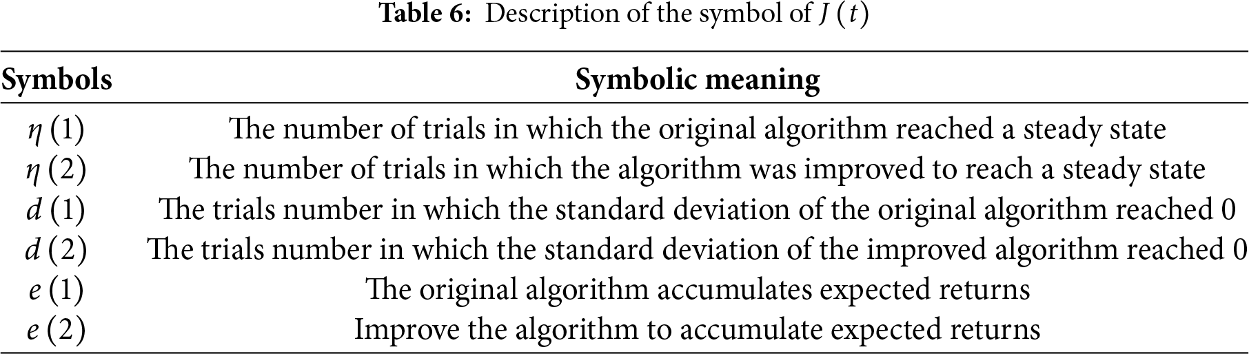
Therefore, the performance evaluation index used in this paper is defined by Formula (10).

J(t)=η(1)−η(2)η(1)+d(1)−d(2)d(1)+e(1)−e(2)e(1)3×100%(10)

Table 6 illustrates the meaning of the symbols in (10).

4  Experiments

4.1 Simulation Environment

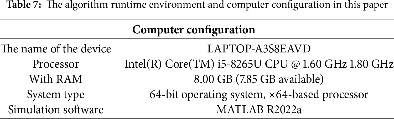
The algorithm runtime environment and computer configuration in this document are shown in Table 7.

Three MATLAB-designed raster map environments of varying complexity were implemented to evaluate the IQL algorithm’s performance in route planning. These environments simulate real-world robot path planning, with each cell representing a potential robot position. Black grids denote obstacles, while white grids represent navigable paths, providing a clear framework for algorithm development and testing.

Fig. 10a represents a low-dimensional environment with few obstacles, where the robot can quickly find the optimal path between the start and end points. This setup is used to test the basic functionality and learning efficiency of the IQL algorithm.

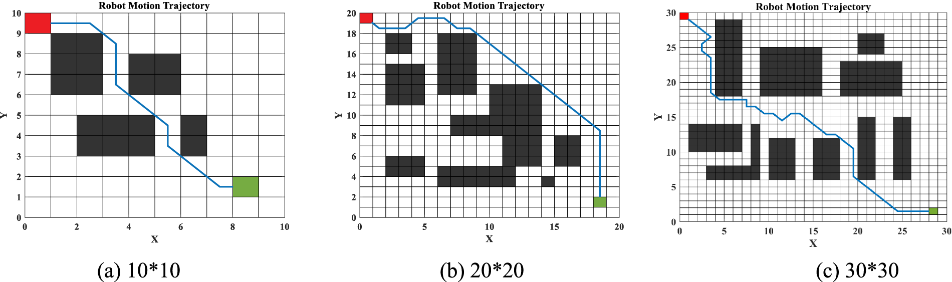
Figure 10: Raster map environment

Fig. 10b is of medium dimensionality and has a more complex structure, including more black grids. This environment allows for the testing of the route planning ability and computational efficiency of the IQL algorithms in the face of more complex situations.

Fig. 10c is a high-dimensional complex map designed with a large number of obstacles. This environment simulates a challenging navigation task in the real world. It is used to estimate the performance of the IQL algorithm in dealing with elaborate environments, especially in planning speed and obstacle avoidance.

A series of simulation experiments in three different dimensional raster map environments were conducted to compare the performance of the IQL algorithm with traditional Q-learning and other algorithms. This comprehensive evaluation highlights the practical effects and potential application value of the proposed optimization methodology for path planning problems.

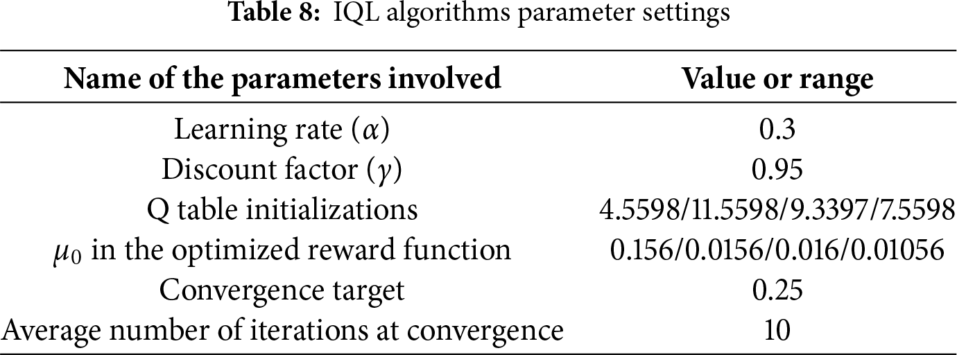
Basic parameter settings chosen for this experiment are presented in Table 8.

4.2 Algorithm Validation

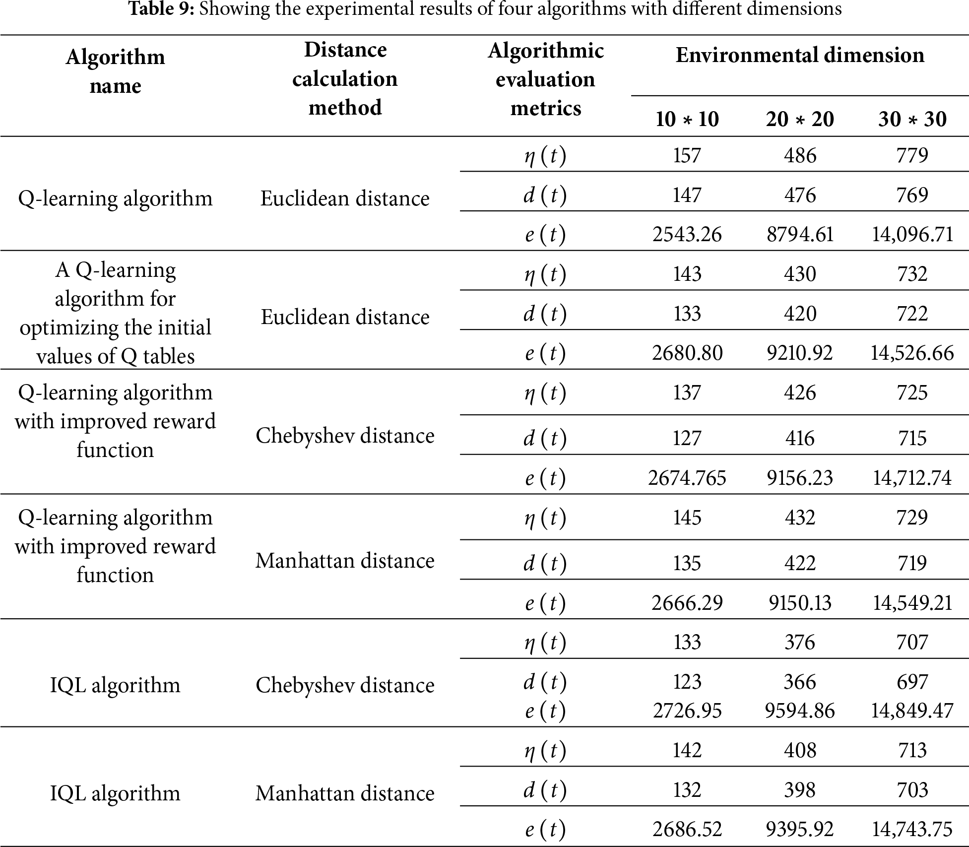
In this section, the following four algorithms are tested in each of the above three environments:

(a)   Q-learning algorithm.

(b)   A Q-learning algorithm for optimizing the initial values of Q-tables.

(c)   Q-learning algorithm with improved reward function.

(d)   IQL algorithm.

After preliminary experiments and parameter tuning, this study found that the IQL algorithm achieved the best learning and path planning performance when the Q-table was initialized at 9.3397, the parameter ρ0 in the optimized reward function was 0.016, and the distance was computed using the Chebyshev metric. Therefore, this parameter is chosen as the parameter setting of the algorithm in this section to demonstrate the experimental results of this study; all the experiments in this section are conducted with this parameter. Table 9 below demonstrates the experimental results when the Q-table is initialized with a value of 9.3397, ρ0 in the optimized reward function is 0.016, and the distance calculation methods are Chebyshev distance and Manhattan distance.

Overall, the Q-learning algorithm performance is significantly improved for simple scenes in low dimensions and complex maps in higher dimensions.

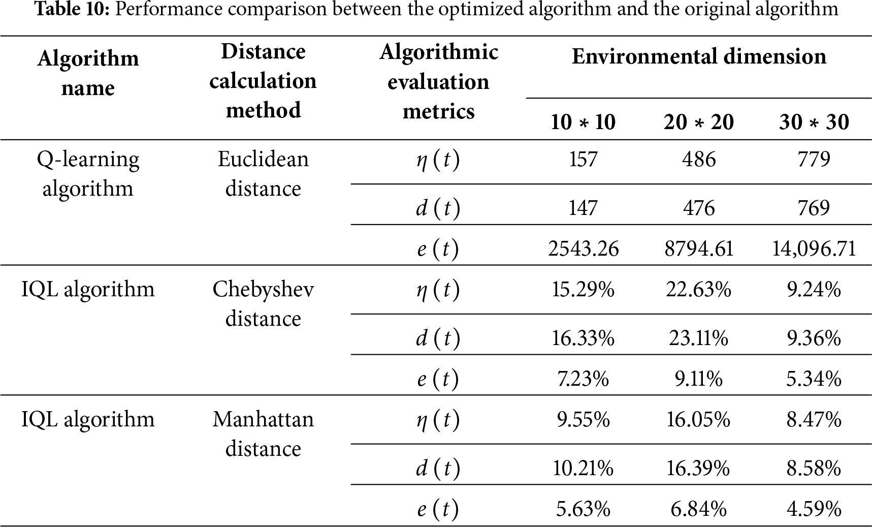
In the low-dimensional raster map environments of size 10 ∗ 10 and 20 ∗ 20, both the number of trials required for convergence and the number needed for the standard deviation to reach zero were significantly reduced. For the 10 ∗ 10 maps, the IQL algorithm with Chebyshev distance decreased the trials required for convergence by 15.29% and those for achieving a standard deviation of zero by 16.33%. The optimized algorithm can achieve a higher expected return in the initial state after convergence when the expected return increases by 7.23%. The IQL algorithm based on Chebyshev distance requires 22.63% fewer trials to reach a steady state or convergence and 23.11% fewer trials to get a standard deviation 0 in a 20 ∗ 20 raster map. In contrast, the optimized algorithm can achieve higher expected returns in the initial state after convergence, which is an increase of 9.11% in the expected returns. The performance of the algorithm in a 20 ∗ 20 raster map is better than that in a 10 ∗ 10 raster map, which is an increase of 7.23%. The algorithm performs better in the 20 ∗ 20 raster map than in the 10 ∗ 10 map, demonstrating its ability to scale to larger problems and handle increased environmental complexity. In the 30 ∗ 30 map, performance continues to improve, but the number of trials required for convergence stabilizes, and the reductions in standard deviation and the increase in expected return become smaller. Taking the Chebyshev distance based IQL algorithm in a 30 ∗ 30 raster map as an example, the trial number demanded to gain a steady state or convergence decreases by 9.24%. The trial number demanded to attain a standard deviation of 0 decreases by 9.36%. In contrast, the optimized algorithm can achieve higher expected returns in the initial state after convergence when the expected return increases by 5.34%.

After careful analysis and comparison, this paper confirms the remarkable effectiveness of the optimization strategy. The IQL algorithm not only achieves a breakthrough in learning efficiency but also demonstrates significant dominance in terms of accuracy and stability of path planning. These results are validated through rigorous experiments, which included tests in multiple complex environments and comparative analyses with the original algorithm and other existing algorithms. Table 10 below demonstrates the optimized algorithm performance compared with the original algorithm.

4.3 Algorithm Comparison

This section highlights the advantages of the IQL algorithm by comparing it with the FIQL, PP-Q-Learning-based CPP (PP-QL-based CPP), DFQL, and QMABC algorithms. The comparison follows these steps.

Step1: Clarify the purpose of the comparison.

This program aims to compare the performance of different algorithms in 10 ∗ 10 and 20 ∗ 20 raster environments. By examining these scenarios, we can understand the variation in efficiency and effectiveness of three algorithms across different raster map sizes.

Step2: Selection of benchmarking algorithms.

This section compares the IQL algorithm with the FIQL, PP-QL-based CPP, DFQL, and QMABC algorithms. These comparison algorithms are all variants of Q-learning that use different approaches to enhance learning speed and performance. This comparison demonstrates the superiority of the IQL algorithm.

Step3: Algorithm performance evaluation metrics.

Evaluation metrics are crucial for measuring algorithm performance. We will use three metrics from Section Methods: the number of trials X under consistent iterations (η(t)), the number of trials where the standard deviation reaches 0 (d(t)), and the expected return after convergence (e(t)). All algorithms must be run under the same conditions and tested on the same dataset. Additionally, the performance of each metric should be recorded and statistically analyzed to identify the best-performing algorithm for the given scenario.

Step4: Comparative analysis of algorithms.

Table 11 compared the experimental results of the Q-learning algorithm with the IQL algorithm, the FIQL algorithm, the PP-QL-based CPP algorithm, the DFQL algorithm, and the QMABC algorithm.

The IQL algorithm exhibited substantial performance advantages under both the 10 ∗ 10 grid map and the 20 ∗ 20 grid map conditions. To illustrate this, consider the evaluation metric of the number of trials required to reach a steady state with zero standard deviation. In the 10 ∗ 10 grid environment, the IQL algorithm, FIQL algorithm, and CPP algorithm based on PP-Q-learning achieved the steady state with zero standard deviation in 16.33%, 8.84%, and 10.88% fewer trials, respectively, compared to the traditional Q-learning algorithm. In the 20 ∗ 20 grid environment, the enhanced IQL algorithm exhibited a substantial performance enhancement of 10.88%. A comparison of the three algorithms with the traditional Q-learning algorithm in the 20 × 20 grid environment reveals that the number of trials required for the three algorithms to reach a zero standard deviation steady state decreased by 23.11%, 10.50%, and 11.34%, respectively. It is evident that the IQL algorithm demonstrates the most rapid convergence speed and the highest level of stability among the three algorithms under consideration. It has been demonstrated that the system learns and executes tasks with greater efficiency in the same environment, delivering optimal algorithmic performance. In addition, the IQL algorithm exhibits remarkable performance in the other two evaluation metrics. It has been demonstrated that IQL attains the most rapid convergence speed and the highest stability, thus facilitating more effective task learning and execution while delivering the optimum overall performance.

The graphs illustrate the results of experiments in two different raster environments, comparing the FIQL algorithm, the PP-QL-based CPP algorithm, and the improved IQL algorithm. This section focuses on the number of trials where the standard deviation reaches 0, a key stability and convergence speed metric. A smaller standard deviation indicates more stable data; a standard deviation 0 means complete stability. The IQL algorithm converges faster than the other two algorithms in both raster environments as shown in Fig. 11.

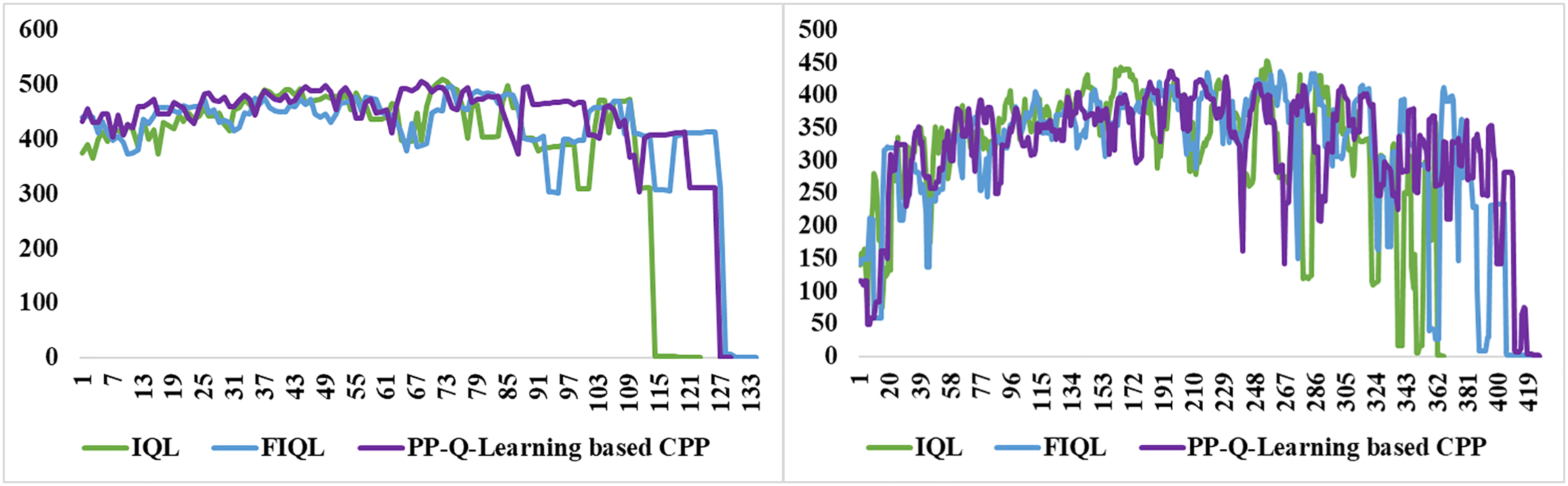
Figure 11: Comparison of the number of trials in which the standard deviation of the three different algorithms reaches 0 for two types of raster environments

This quick convergence is valuable for practical applications as it reduces the time needed for learning and planning. The IQL algorithm not only converges faster but also achieves better final performance.

The IQL algorithm enhances learning efficiency and task performance within the same environment, boosting overall performance, which is crucial for tackling more complex and larger-scale problems. In summary, its performance in a raster environment demonstrates its effectiveness in improving learning efficiency, stability, and outcomes, offering valuable insights for future algorithm design and optimization in similar settings.

4.4 Discussion

Our work proposes an optimized algorithm that improves Q-table initialization and refines the reward function, enabling faster and more efficient strategy development in complex environments by reducing unnecessary trial and error. This approach shows broad applicability across various raster map environments, consistently improving the IQL algorithm’s ability to navigate high-dimensional maps with numerous obstacles. Experimental results confirm the algorithm’s stability and reliability, validating its effectiveness in path planning through both theoretical and empirical analysis.

The IQL algorithm shows enhanced performance across all map dimensions. In low-dimensional maps, it efficiently guides the agent to avoid obstacles and find the optimal path, significantly outperforming traditional Q-learning. Even in more complex 30 ∗ 30 maps, the algorithm reduces trials needed for convergence and increases expected returns, consistently providing better stability, faster convergence, and more effective pathfinding across all tested dimensions. While the present study concentrates on a 30 ∗ 30 grid environment, subsequent research will extend to larger scale scenarios (e.g., 50 ∗ 50) and dynamic obstacle distributions to further validate the scalability of the algorithm for real-world applications.

These findings have significant implications for practical applications, particularly in the operation of autonomous robots or vehicles in complex and dynamic environments. Although the IQL algorithm demonstrates superior stability and convergence speed under certain conditions, further optimization is needed to enhance its adaptability and decision-making speed in highly complex, dynamic environments. Although the PACO-based initialization and UCH mechanism improve convergence and stability, they also increase algorithmic complexity and computational cost, which may limit applicability in large-scale maps or resource-constrained robotic platforms. Future research should focus on improving the algorithm’s robustness in such environments to ensure that autonomous systems can achieve efficient and stable path planning across various real-world scenarios. This will not only increase the practical value of the algorithm but also advance the development of autonomous robotics and vehicle technologies. In addition, this work compared IQL mainly with classical and enhanced Q-learning methods. Deep reinforcement learning approaches such as DQN and DDQN were not included, as our study focused on discrete raster environments. Future research will consider these methods in dynamic and multi-agent settings to further assess IQL’s adaptability.

5  Conclusion

We present an IQL algorithm that leverages the PACO algorithm to optimize initial Q-table values, enabling the agent to quickly adapt and select optimal paths. This approach addresses key challenges in path planning within complex environments, including slow convergence, local optimization issues, and the need for precise environment modeling. Furthermore, we incorporated a UCH reward function mechanism to alleviate reward function sparsity, reduce exploration difficulties, and enhance reward evaluation. Compared to traditional methods, the IQL algorithm significantly improves performance, speed, and accuracy, effectively meeting the demands of path planning and obstacle avoidance. Our results indicate that the model demonstrates strong generalization capabilities across various scenarios. The experiments in this paper are based on static grid environments, and the IQL algorithm will be subsequently extended to scenarios with higher dimensional environments, dynamic obstacles, partially observable and multi-intelligentsia in order to validate its robustness and scalability, and to increase the value of its application in real robot navigation.

Acknowledgement: We would like to express our gratitude to the School of Science at Liaoning Technical University for providing computing resources.

Funding Statement: Financial supports from the National Natural Science Foundation of China (Grant No. 52374123 & 51974144), Project of Liaoning Provincial Department of Education (Grant No. LJKZ0340), and Liaoning Revitalization Talents Program (Grant No. XLYC2211085) are greatly acknowledged.

Author Contributions: Ruiyang Wang: Conceptualization, Data curation, Formal analysis, Investigation, Methodology, Writing—original draft, Writing—review & editing. Wei Liu and Guangwei Liu: Funding acquisition, Project administration, Resources, Software, Supervision, Validation, Visualization, Writing—review & editing. All authors reviewed the results and approved the final version of the manuscript.

Availability of Data and Materials: Data available on request from the authors.

Ethics Approval: No ethical approval was required for this study, as it did not involve human participants or animals.

Conflicts of Interest: The authors declare no conflicts of interest to report regarding the present study.

References

1. Alatise MB, Hancke GP. A review on challenges of autonomous mobile robot and sensor fusion methods. IEEE Access. 2020;8:39830–46. doi:10.1109/access.2020.2975643. [Google Scholar] [CrossRef]

2. Rubio F, Valero F, Llopis-Albert C. A review of mobile robots: concepts, methods, theoretical framework, and applications. Int J Adv Rob Syst. 2019;16(2):1729881419839596. doi:10.1177/1729881419839596. [Google Scholar] [CrossRef]

3. Xiao XS, Liu B, Warnell G. Motion planning and control for mobile robot navigation using machine learning: a survey. Auton Robot. 2022;46(5):569–97. doi:10.1007/s10514-022-10039-8. [Google Scholar] [CrossRef]

4. Teng S, Hu X, Deng P, Li B, Li Y, Ai Y, et al. Motion planning for autonomous driving: the state of the art and future perspectives. IEEE Trans Intell Veh. 2023;8(6):3692–711. doi:10.1109/tiv.2023.3274536. [Google Scholar] [CrossRef]

5. Chu Z, Wang F, Lei T, Luo C. Path planning based on deep reinforcement learning for autonomous underwater vehicles under ocean current disturbance. IEEE Trans Intell Veh. 2023;8(1):108–20. doi:10.1109/TIV.2022.3153352. [Google Scholar] [CrossRef]

6. Lin Z, Wang H, Chen T, Jiang Y, Jiang J, Chen Y. A reverse path planning approach for enhanced performance of multi-degree-of-freedom industrial manipulators. Comput Model Eng Sci. 2024;139(2):1357–79. doi:10.32604/cmes.2023.045990. [Google Scholar] [CrossRef]

7. Sun YH, Fang M, Su YX. AGV path planning based on improved dijkstra algorithm. J Phys Conf Ser. 2020;1746(1):22–3. doi:10.1088/1742-6596/1746/1/012052. [Google Scholar] [CrossRef]

8. Parimala M, Broumi S, Prakash K. Bellman-ford algorithm for solving shortest path problem of a net-work under picture fuzzy environment. Compl Intell Syst. 2021;7(5):2373–81. doi:10.1007/s40747-021-00430-w. [Google Scholar] [CrossRef]

9. Tang G, Tang C, Claramunt C, Hu X, Zhou P. Geometric A-star algorithm: an improved A-star algorithm for AGV path planning in a port environment. IEEE Access. 2021;9:59196–210. doi:10.1109/access.2021.3070054. [Google Scholar] [CrossRef]

10. Wang J, Chi W, Li C, Wang C, Meng MQ. Neural RRT*: learning-based optimal path planning. IEEE Trans Automat Sci Eng. 2020;17(4):1748–58. doi:10.1109/tase.2020.2976560. [Google Scholar] [CrossRef]

11. Chen Y, Bai G, Zhan Y, Hu X, Liu J. Path planning and obstacle avoiding of the USV based on improved ACO-APF hybrid algorithm with adaptive early-warning. IEEE Access. 2021;9:40728–42. doi:10.1109/access.2021.3062375. [Google Scholar] [CrossRef]

12. Song B, Wang Z, Zou L. An improved PSO algorithm for smooth path planning of mobile robots using continuous high-degree Bezier curve. Appl Soft Comput. 2021;100(1):106960. doi:10.1016/j.asoc.2020.106960. [Google Scholar] [CrossRef]

13. Li Y, Dong D, Guo X. Mobile robot path planning based on improved genetic algorithm with A-star heuristic method. In: 2020 IEEE 9th Joint International Information Technology and Artificial Intelligence Conference (ITAIC); 2020 Dec 11–13; Chongqing, China. p. 11–3. doi:10.1109/itaic49862.2020.9338968. [Google Scholar] [CrossRef]

14. Wei X, Zhang Y, Song H, Qin H, Zhao G. Research on evacuation path planning based on improved sparrow search algorithm. Comput Model Eng Sci. 2024;139(2):1295–316. doi:10.32604/cmes.2023.045096. [Google Scholar] [CrossRef]

15. Wang B, Liu Z, Li Q, Prorok A. Mobile robot path planning in dynamic environments through globally guided reinforcement learning. IEEE Robot Autom Lett. 2020;5(4):6932–9. doi:10.1109/LRA.2020.3026638. [Google Scholar] [CrossRef]

16. Liu Z, Chen B, Zhou H, Koushik G, Hebert M, Zhao D. MAPPER: multi-agent path planning with evolutionary reinforcement learning in mixed dynamic environments. In: 2020 IEEE/RSJ International Conference on Intelligent Robots and Systems (IROS); 2020 Oct 24–2021 Jan 24; Las Vegas, NV, USA. p. 11748–54. doi:10.1109/iros45743.2020.9340876. [Google Scholar] [CrossRef]

17. He L, Aouf N, Song B. Explainable deep reinforcement learning for UAV autonomous path planning. Aerosp Sci Technol. 2021;118(7):107052. doi:10.1016/j.ast.2021.107052. [Google Scholar] [CrossRef]

18. Theile M, Bayerlein H, Nai R, Gesbert D, Caccamo M. UAV path planning using global and local map information with deep reinforcement learning. In: 2021 20th International Conference on Advanced Robotics (ICAR); 2021 Dec 6–10; Ljubljana, Slovenia. p. 6–10. doi:10.1109/icar53236.2021.9659413. [Google Scholar] [CrossRef]

19. Chen P, Pei J, Lu W, Li M. A deep reinforcement learning based method for real-time path planning and dynamic obstacle avoidance. Neurocomputing. 2022;497(8):64–75. doi:10.1016/j.neucom.2022.05.006. [Google Scholar] [CrossRef]

20. Liu Q, Shi L, Sun L, Li J, Ding M, Shu FS. Path planning for UAV-mounted mobile edge computing with deep reinforcement learning. IEEE Trans Veh Technol. 2020;69(5):5723–8. doi:10.1109/tvt.2020.2982508. [Google Scholar] [CrossRef]

21. Hong D, Lee S, Cho YH, Baek D, Kim J, Chang N. Energy-efficient online path planning of multiple drones using reinforcement learning. IEEE Trans Veh Technol. 2021;70(10):9725–40. doi:10.1109/TVT.2021.3102589. [Google Scholar] [CrossRef]

22. Li L, Wu D, Huang Y, Yuan ZM. A path planning strategy unified with a COLREGS collision avoidance function based on deep reinforcement learning and artificial potential field. Appl Ocean Res. 2021;113(27):102759. doi:10.1016/j.apor.2021.102759. [Google Scholar] [CrossRef]

23. Xu X, Cai P, Ahmed Z, Yellapu VS, Zhang W. Path planning and dynamic collision avoidance algorithm under COLREGs via deep reinforcement learning. Neurocomputing. 2022;468(1):181–97. doi:10.1016/j.neucom.2021.09.071. [Google Scholar] [CrossRef]

24. Hu H, Yang X, Xiao S, Wang F. Anti-conflict AGV path planning in automated container terminals based on multi-agent reinforcement learning. Int J Prod Res. 2023;61(1):65–80. doi:10.1080/00207543.2021.1998695. [Google Scholar] [CrossRef]

25. Josef S, Degani A. Deep reinforcement learning for safe local planning of a ground vehicle in unknown rough terrain. IEEE Robot Autom Lett. 2020;5(4):6748–55. doi:10.1109/LRA.2020.3011912. [Google Scholar] [CrossRef]

26. Hao B, Du H, Yan Z. A path planning approach for unmanned surface vehicles based on dynamic and fast Q-learning. Ocean Eng. 2023;270(4):113632. doi:10.1016/j.oceaneng.2023.113632. [Google Scholar] [CrossRef]

27. Maoudj A, Hentout A. Optimal path planning approach based on Q-learning algorithm for mobile robots. Appl Soft Comput. 2020;97(2):106796. doi:10.1016/j.asoc.2020.106796. [Google Scholar] [CrossRef]

28. Low ES, Ong P, Cheah KC. Solving the optimal path planning of a mobile robot using improved Q-learning. Robot Auton Syst. 2019;115(3):143–61. doi:10.1016/j.robot.2019.02.013. [Google Scholar] [CrossRef]

29. Hao B, Zhao J, Du H, Wang Q, Yuan Q, Zhao S. A search and rescue robot search method based on flower pollination algorithm and Q-learning fusi on algorithm. PLoS One. 2023;18(3):e0283751. doi:10.1371/journal.pone.0283751. [Google Scholar] [PubMed] [CrossRef]

30. Ni X, Hu W, Fan Q, Cui Y, Qi C. A Q-learning based multi-strategy integrated artificial bee colony algorithm with application in unmanned vehicle path planning. Expert Syst Appl. 2024;236(4):121303. doi:10.1016/j.eswa.2023.121303. [Google Scholar] [CrossRef]

31. Das PK, Behera HS, Panigrahi BK. Intelligent-based multi-robot path planning inspired by improved classical Q-learning and improved particle swarm optimization with perturbed velocity. Eng Sci Technol Int J. 2016;19(1):651–69. doi:10.1016/j.jestch.2015.09.009. [Google Scholar] [CrossRef]

32. Low ES, Ong P, Low CY. A modified Q-learning path planning approach using distortion concept and optimization in dynamic environment for autonomous mobile robot. Comput Ind Eng. 2023;181(6):109338. doi:10.1016/j.cie.2023.109338. [Google Scholar] [CrossRef]

33. Puente-Castro A, Rivero D, Pedrosa E, Pereira A, Lau N, Fernandez-Blanco E. Q-learning based system for path planning with unmanned aerial vehicles swarms in obstacle environments. Expert Syst Appl. 2024;235(2):121240. doi:10.1016/j.eswa.2023.121240. [Google Scholar] [CrossRef]

34. Yu X, Luo W. Reinforcement learning-based multi-strategy cuckoo search algorithm for 3D UAV path planning. Expert Syst Appl. 2023;223(4):119910. doi:10.1016/j.eswa.2023.119910. [Google Scholar] [CrossRef]

35. Kulathunga G. A reinforcement learning based path planning approach in 3D environment. Procedia Comput Sci. 2022;212(1):152–60. doi:10.1016/j.procs.2022.10.217. [Google Scholar] [CrossRef]

36. Lee G, Kim K, Jang J. Real-time path planning of controllable UAV by subgoals using goal-conditioned reinforcement learning. Appl Soft Comput. 2023;146(6):110660. doi:10.1016/j.asoc.2023.110660. [Google Scholar] [CrossRef]

37. Petrik J, Bambach M. Reinforcement learning and optimization based path planning for thin-walled structures in wire arc additive manufacturing. J Manuf Process. 2023;93(6):75–89. doi:10.1016/j.jmapro.2023.03.013. [Google Scholar] [CrossRef]

38. Zhao M, Lu H, Yang S, Guo Y, Guo F. A fast robot path planning algorithm based on bidirectional associative learning. Comput Ind Eng. 2021;155:107173. doi:10.1016/j.cie.2021.107173. [Google Scholar] [CrossRef]

39. Ladosz P, Weng L, Kim M, Oh H. Exploration in deep reinforcement learning: a survey. Inf Fusion. 2022;85(7540):1–22. doi:10.1016/j.inffus.2022.03.003. [Google Scholar] [CrossRef]

40. Zhang M, Cai W, Pang L. Predator-prey reward based Q-learning coverage path planning for mobile robot. IEEE Access. 2023;11(5):29673–83. doi:10.1109/access.2023.3255007. [Google Scholar] [CrossRef]

41. Ding Z, Huang Y, Yuan H, Dong H. Introduction to reinforcement learning. In: Deep reinforcement learning. Singapore: Springer; 2020. p. 47–123. doi:10.1007/978-981-15-4095-0_2. [Google Scholar] [CrossRef]

42. Li W, Wang J, Li L, Peng Q, Huang W, Chen X, et al. Secure and reliable downlink transmission for energy-efficient user-centric ultra-dense networks: an accelerated DRL approach. IEEE Trans Veh Technol. 2021;70(9):8978–92. doi:10.1109/tvt.2021.3098978. [Google Scholar] [CrossRef]

43. Tan T, Xie H, Feng L. Q-learning with heterogeneous update strategy. Inf Sci. 2024;656(1):119902. doi:10.1016/j.ins.2023.119902. [Google Scholar] [CrossRef]

44. George Karimpanal T, Le H, Abdolshah M, Rana S, Gupta S, Tran T, et al. Balanced Q-learning: combining the influence of optimistic and pessimistic targets. Artif Intell. 2023;325(7540):104021. doi:10.1016/j.artint.2023.104021. [Google Scholar] [CrossRef]

45. Li X, Liang X, Wang X, Wang R, Shu L, Xu W. Deep reinforcement learning for optimal rescue path planning in uncertain and complex urban pluvial flood scenarios. Appl Soft Comput. 2023;144:110543. doi:10.1016/j.asoc.2023.110543. [Google Scholar] [CrossRef]

46. Low ES, Ong P, Low CY. An empirical evaluation of Q-learning in autonomous mobile robots in static and dynamic environments using simulation. Decis Anal J. 2023;8:100314. doi:10.1016/j.dajour.2023.100314. [Google Scholar] [CrossRef]

47. García M, López N, Rodríguez I. A full process algebraic representation of ant colony optimization. Inf Sci. 2024;658(3):120025. doi:10.1016/j.ins.2023.120025. [Google Scholar] [CrossRef]

48. Tadaros M, Kyriakakis NA. A hybrid clustered ant colony optimization approach for the hierarchical multi-switch multi-echelon vehicle routing problem with service times. Comput Ind Eng. 2024;190(2):110040. doi:10.1016/j.cie.2024.110040. [Google Scholar] [CrossRef]

49. Li T, Zuo E, Chen C, Chen C, Zhong J, Yan J, et al. Gaussian distribution resampling via Chebyshev distance for food computing. Appl Soft Comput. 2024;150(5):111103. doi:10.1016/j.asoc.2023.111103. [Google Scholar] [CrossRef]

50. Wang C, Yang J, Zhang B. A fault diagnosis method using improved prototypical network and weighting similarity-Manhattan distance with insufficient noisy data. Measurement. 2024;226(7):114171. doi:10.1016/j.measurement.2024.114171. [Google Scholar] [CrossRef]