Hesitation Analysis with Kullback Leibler Divergence and Its Calculation on Temporal Data

1  Introduction

The decision-making problem has been extensively explored across diverse areas including management, economics, and industry [1–3]. Additionally, multi-criteria problems were addressed continuously by the numerous researchers as well [4–6]. Previous studies also focused on enhancing their precision and generalizability for practical applications by developing score functions. Consequently, researchers have proposed various approaches to address the complexities in score function design [7–10]. In addressing the challenge of score function development, we managed hesitation through intuitionistic fuzzy sets (IFSs) [11–13]. However, dissatisfaction with decision outcomes persists due to similarity in decision values and instances of indecision [1,2,8,9]. Hence, we faced the following issues:

•   Data on hesitation are limited, affecting the balance between supporting and dissenting responses.

•   A more rational analysis of hesitation, including its variability, is necessary.

Research in decision and classification has also leveraged granular computing, a framework pioneered by Zadeh [14] and Bargiela and Pedrycz [15]. Continuous research has been conducted by many researchers [16–18]. While granular computing has shown promise in recognition and decision applications, its performance is less consistent when handling large datasets. Although hesitation is defined within the IFS framework, few studies have thoroughly investigated its role in decision-making. Recently, hesitation analysis has been applied in pattern recognition, which is derived based on information distribution [12]. The research evaluates both synthetic numerical examples via granular computing and a cognitive viewpoint was also demonstrated [17]. In this context, we consider Kullback-Leibler (KL) divergence as the tool to investigate the effect of hesitation within the IFS framework [19]. Different from fuzzy sets (FSs), IFSs have a challenge in treating hesitation [11]. Furthermore, KL divergence needs an additional complement to use as the distance measure because of the non-symmetric property [20,21]. IFS Knowledge categorizes information into affirmative, dissent, and abstention, represented by μ(x), ν(x), and π(x) in IFS notation. KL divergence helps quantify the probabilistic distance between μ(x), and ν(x), despite lacking symmetry and triangular inequality properties [12,13]. Specifically, even the same hesitation supportive information–μ(x)—has different support for the alternative, so the hesitation analysis is decisive in the decision-making. Building on prior research, decision-making methods have been applied across diverse fields such as business management, engineering, and social sciences [1,2,4]. With its applications across domains, the KL divergence can also be integrated into artificial intelligence (AI) alongside cross-entropy (CE) [22]. A fundamental limitation, however, is that it requires predefined probability distributions, reducing adaptability for real-time data integration. By utilizing affirmative, dissent, and abstention information, hesitation calculations can be applied to specific decision scenarios, such as election outcomes. Here, achieving over 50% support serves as the decision threshold. Using the numerical difference between affirmative and dissent values, hesitation metric values can be derived, providing more reliable predictions when aligned with actual data. Furthermore, the freshness and accuracy of the sensing data are critical to the sensing systems. Hence, research has been conducted on information entropy optimization. With the help of information theory, hesitation calculation is proposed in this research. Furthermore, accumulated information also plays a crucial role in decision-making from the common sense. Applying this approach to Korean congressional election data [23], hesitation calculations are analyzed based on seven census polls that indicate support and dissent for a specific candidate. In this regard, two analytical approaches are proposed in the research.

•   Hesitation calculation is based on the affirmative and dissenting information. So we proposed hesitation calculation with the help of Kullback-Leibler divergence illustrated in information theory [19,24].

•   Data are updated using the conditional probability, and the calculation results are illustrated with the decision results.

The calculation of the degree of hesitation is based on the deviation of the support ratio from 50% using the KL divergence. The hesitation degree is further assessed by the difference between the supportive and opposing degrees, where the supportive trend is represented by its derivative. Additionally, this decision-making framework incorporates prior information and likelihood functions to determine posterior information, integrating recent data. An example is presented to validate the proposed methodologies: a Korean election analysis that predicts results based on supportive and dissenting ratios, using updated consensus data before the election date. Affirmative and dissenting opinions towards candidates are modeled using IFSs, while the remaining ratios represent middle-class opinions. Calculations demonstrate that this decision yields meaningful insights compared to existing methodologies.

In decision-making problems, to address complex and uncertain circumstances, three-dimensional divergence-based decision making (DM) has been proposed to enhance the discrimination of information [25]. Additionally, to evaluate complex alternatives under uncertainty, vagueness, and inconsistent linguistic expressions, a novel multi-criteria group decision-making (MCGDM) approach was also proposed, which is grounded in cubic sets, and integrates Minkowski-based distance measures and entropy-based weighting strategies [26].

The rest of the study is structured as follows: Section 2 briefly introduces hesitation and KL divergence. It includes an overview of hesitation from both supportive and opposing perspectives and the KL divergence calculation method. Section 3 outlines the hesitation calculation based on the KL divergence and temporal data analysis. Section 4 applies the KL-divergence to the Korean congressional election, where two approaches are used: hesitation calculation with the KL divergence and temporal data updates with conditional probability. The results are then discussed—finally, Section 5 offers concluding remarks.

2  Preliminaries

Brief descriptions of IFSs and KL divergence are illustrated in this section. Especially, the role of hesitation–π(x)—and relations with membership and non-membership are emphasized.

2.1 Hesitation in Intuitionistic Fuzzy Sets

According to IFS definitions, hesitation degree is determined as follows [11]:

π(x)=1−μ(x)−ν(x)

It is expressed by the difference between the whole information (totally one) and the sum of membership and non-membership functions, where μ(x) and ν(x) denote membership(affirmative) and non-membership (dissent) functions on x∈X, respectively. X is universe of discourse accordingly. Hence, the following definition of the IFSs is applied in the existing research [11].

Definition 1. IFSs I for the universe of discourse X={x1,x2,…,xn} is defined as follows:

I={⟨x,μI(x),νI(x)⟩|x∈X,μI(x),νI(x)∈[0,1],0≤μI(x)+νI(x)≤1}.

Given the values of μI(x) and νI(x): representing affirmative and dissent, the following preference can be stated in Fig. 1. From Fig. 1, it is observed that items A and B share an equal hesitation index of –0.1. However, their affirmative and dissent characteristics differ; affirmatives are 0.8 and 0.2 for A and B, respectively. KL divergence analysis proves insightful for decision-making, especially in binary contexts, where a threshold of 0.5 facilitates decisions. Calculation results demonstrate that for A, the KL divergence of A to decision boundary [9].

D(μ(x)‖0.5)=μ(x)log2μ(x)0.5,(1)

calculation result satisfies

D(0.8‖0.5)=0.8log20.80.5=0.5425.

Figure 1: Affirmative and dissent representation of A and B

For B, D(0.2‖0.5)=0.2log20.20.5=−0.2644 is obtained. Logarithmic analysis shows that distances greater than 0.5 yield a positive divergence, while those below 0.5 are negative, highlighting distinct interpretations of KL divergence. Even the same hesitation of π(x), this divergence allows for a nuanced understanding of affirmation and dissent in two primary categories: (i) KL divergence between μ(x) and 0.5 (ii) KL divergence from ν(x) and 0.5. From the first one–(i), it is also classified two cases;

•   μ(x)≥0.5; decided with enough, conservative, overwhelm hesitation,

•   μ(x)≤0.5; cannot reach to decision, hesitation is also included.

Dissent opinion can be realized by the calculation between ν(x) and 0.5—calculation of μ(x)≤0.5. It also has two types: ν(x)≥0.5 and ν(x)≤0.5. Calculation results are the same result with respect to the disagreement. Hesitation is also included in each case, but dissent is overwhelmed when ν(x)>0.5. Fig. 1 indicates that IFS A is more concrete in the decision than B. However, it is given from the common concept. The KL divergence calculation, is calculated in the following subsection. A more decisive opinion becomes the standard from 0.5 whether it is affirmative or dissent.

2.2 KL Divergence Calculation

In the binary decision scenarios, decisions are concluded when affirmation exceeds 0.5. For competitive candidates, hesitation may be decisive, warranting deeper analysis. Log scale values—log2x—diminish rapidly for x<1, and stabilize for x>1. Values of μ(x) and ν(x) include hesitation, except when at boundary values (0 or 1). Using KL divergence, as formulated in Eq. (1), we capture hesitation information relative to 0.5. For example, the KL divergences of minor opinions of A and B to 0.5 in Fig. 1 are given by the following Equations.

D(ν(x)‖0.5)=ν(x)log2ν(x)0.5,for ν(x)=0.1,(2)

and

D(μ(x)‖0.5)=μ(x)log2μ(x)0.5,where μ(x)=0.2.(3)

By the calculation, Eqs. (2) and (3) are −0.2322 and −0.2644, respectively. Contrary opinions of A and B are illustrated by the major concerns; for A,

D(μ(x)‖0.5)=μ(x)log20.80.5,for μ(x)=0.8,

and for B,

D(ν(x)‖0.5)=ν(x)log2ν(x)0.5,for ν(x)=0.7,

calculation results are and respectively. Complete decision opinion is calculated by

D(1‖0.5)=1⋅log210.5=1.

Hence, the hesitation of major opinion represents the distance from the mentioned complete distance; therefore 1−0.5425 or 1−0.3398. Then, it is clear that A in Fig. 1 shows less hesitation for the decision. For the minor opinion, |−0.2322| and |−0.2344| illustrate the distance from the half value 0.5. Then, the hesitation of B is greater than that of A. In this regard, we can notice that B in Fig. 1 shows more hesitation than A. From a heuristic viewpoint, it can be inferred that IFS A has more sensitivity in hesitation than B. These results are insightful for extracting the degree of hesitation. The method of extracting the hesitation degree from μ(x) and ν(x) is evident from the calculation of the mentioned majority and minority opinions.

The answer is obvious from the calculation of the aforementioned major and minor opinions. Specifically, KL divergence under 0.5 probability is non-proportional with respect to the variation of probability. This work presents the KL divergence with respect to –0.5. Explicit KL divergence from distribution to 0.5 is satisfied from the definition as follows:

p⋅log2p0.5=p⋅log2p−p⋅log20.5.

When p(x) approaches to zero and 0.5, its divergence is close to zero.

By derivation with respect to p(x) denotes

log2p+1−log20.5,

and the minimum KL divergence to 0.5 is obtained easily, it is p(x)=0.1839 by the calculation and shown in Fig. 2.

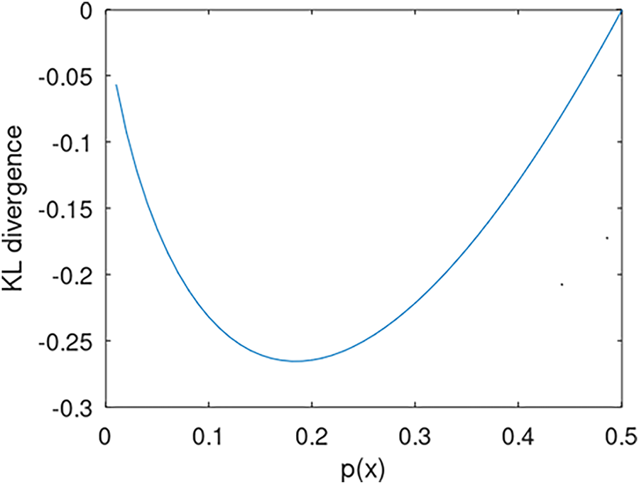
Figure 2: KL divergence with respect to low probability (under 0.5)

3  Hesitation Analysis with KL Divergence

The preliminary results show that hesitation analysis is crucial in decision theory. It offers insights into both analytical derivations and temporal data considerations. This section explores the derivation and temporal characteristics associated with hesitation calculations.

3.1 Hesitation Calculation

Hesitation is estimated by measuring how far the support or dissent deviates from the 0.5 decision threshold. As observed in Fig. 2, the KL divergence reveals a hesitation distance of 0.5. This value stems from the relation between μ(x) and ν(x) each less than 0.5 which are μ(x),ν(x)<0.5. It is clear from Fig. 1, ν(x)=0.1 of A and μ(x)=0.2 of B, so they need to pass hesitation to reach 0.5.

In this regard, we can find the hesitation roughly by the relation from μ(x)=0.8 of A, and ν(x)=0.7 of B to 0.5. However, KL divergence does not represent a standard distance measure; the symmetry property is not satisfied. Modified KL divergence, adapted from Eq. (4), quantifies this deviation. Its nonlinearity reflects how sensitive decisions are near the threshold. From previous findings [19],

dH(p(x))=12{D(p(x)‖0.5))+D(0.5‖p(x))}(4)

dH(p(x)) is positive, but not linear. However, it can approximate hesitation distance relative to μ(x) and ν(x). Examples of the difference between dissent and affirmative to average value can be expressed as dL=d(ν(x))−d(μ(x)). That is the difference between minor and major opinion. For instance, the hesitation distance for A in Fig. 1 can be calculated by examining the deviation.

dL=12{D(0.1‖0.5)+D(0.5‖0.1)−D(0.8‖0.5)−D(0.5‖0.8)}=12{0.1log2(1/5)+0.5log2(5)−0.8log2(8/5)−0.5log2(5/8)}=0.3626.

From the viewpoint of B, the hesitation distance is expressed as

dL=d(μ(x))−d(ν(x))=12{D(0.2‖0.5)+D(0.5‖0.2)−D(0.7‖0.5)−D(0.5‖0.7)}=12{0.2log2(2/5)+0.5log2(5/2)−0.7log2(7/5)−0.5log2(5/7)}=0.1497.

The calculation result is not as straightforward as we expected. Another example is considered by the calculation of hesitation distance itself.

A:dH(p(x))=12{D(0.9‖0.8)+D(0.8‖0.9)}=8.4965×10−3,B:dH(p(x))=12{D(0.7‖0.8)+D(0.8‖0.7)}=9.6325×10−3.

From B’s point of view, the results are intriguing and plausible. Despite equivalent hesitation distances in A and B in Fig. 1, KL divergence calculations reflect varying hesitation values, with A requiring more adjustment to reach the 0.5 level than B. Revisiting the KL divergence formulation through Eq. (4), We revisit the KL divergence formulation via Eq. (4) to capture a probabilistic distribution distance by setting p(x)=1, as in the following equation.

d=sgn(p(x))12{D(p(x)‖0.5))+D(0.5‖p(x))},(5)

sgn(p(x))={−1,if p(x)<0.51,if p(x)>0.5.

It is illustrated in Fig. 3.

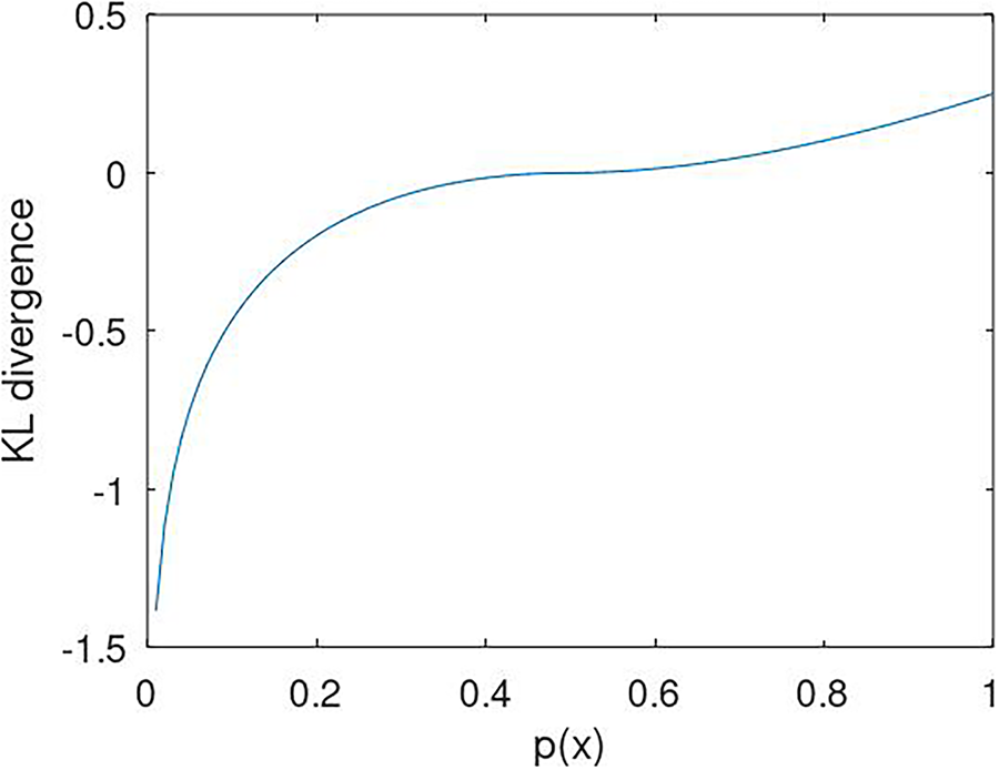
Figure 3: Modified KL divergence Eq. (5) with respect to probability

The variation in divergence over the probability range of 0 to 1 exhibits distinct behavior around the probability near 0.5. Divergence–hesitation–around p(x)=0.5 shows rather flat; low hesitation even it is sensitive. On the other hand, a probability far from 0.5 indicates an abrupt change. Specifically, it is more rapid over p(x)<0.5. It is interesting and not the dual, once the probability is over 0.5, there should be less hesitation. It indicates a rather conservative approach when it is over 0.5–decision bound.

3.2 Hesitation Analysis on Temporal Data

The preceding section detailed the hesitation calculation, highlighting certain limitations regarding temporal data due to constraints in informational variability and trends. Consequently, hesitation is suggested by the sequential expression as dH(k), expressed as:

ds(pk)=sgn(pk(x))12{D(pk(x)‖0.5)+D(0.5‖pk(x))}.(6)

Eq. (6) consists of D(pk(x)‖0.5)) and D(0.5‖pk(x)), so it is the same structure of Eq. (1). Where, pk(x) is the probability at k-th sequential time, and x in universe of discourse X. Calculation of ds(pk(x)) provides instantaneous value, hence it needs to get whether its trend close to the specific value; more specifically close to zero by the repetition. Here, we define as the sufficiency margin to be affirmative when ds(pk(x))>0, and insufficiency margin for ds(pk(x))<0. The value of ds(pk(x)) can become negative or positive for each case. It is noticed that each margin is small and non-sensitive near to pk(x)=0.5 from Fig. 3, it means very competitive situation. However, it is rather sensitive and accelerate when pk(x) is far from 0.5, specifically near to pk(x)=0. From the inspection, Eq. (6) needs to be analyzed its derivative with respect to pk(x), let pk(x)=p for simplicity;

dds(p)dp=12{log2p+log2e−log20.5−0.5plog2e}(7)

It is illustrated in Fig. 4.

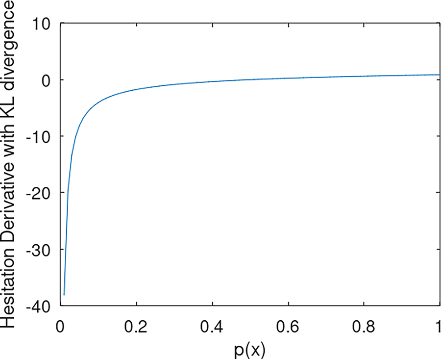
Figure 4: ds(pk) gradient with respect to p(x)

In this draft, simplicity is achieved by defining

dds(p)dpasdsorGrad{ds(p)}.

This definition facilitates the examination of informational hesitation within data updates. With a similar explanation to Fig. 3, hesitation changes drastically when it locates under 0.5.

Subsequently when it is under p(x)=0.1839, it decreases maximally as shown in Fig. 2. Hesitation analysis on temporal data is performed using conditional KL divergence, initially introduced in Eq. (1). To achieve a more robust analysis, this divergence must be reformulated as a conditional divergence that directly incorporates Bayes’ theorem. Specifically, in Eq. (8) redefined using Eq. (9).

D(p(x|y,I)‖p(x|I))=∑x∈Xp(x|y,I)log2p(x|y,I)p(x|I),(8)

p(x|y,I)=p(y|x,I)p(x,I)p(y,I).(9)

A likelihood function and prior function should be assumed or provided to complete the conditional KL divergence. The likelihood function p(y|x,I) of the election process is already illustrated in advance and demonstrated [27]. The data shows that the winning rate varies concerning sustainable high support. In this study, we posit that decisions are influenced by the previous information, not solely the immediately preceding information, a Markov process. Hence, the probability of the first decision x is expressed as p(x|y1), p(x|y1,y2), and so forth. Using Bayes’ theorem, these probabilities are compared by

p(x|y1)=p(x∩y1)p(y1)andp(x|y1,y2)=p(x∩y1∩y2)p(y1∩y2),

are repeated after the information is updated.

Fig. 5 presents a summary of the hesitation analysis using the KL divergence. First, possible information needs to be transformed into IFS data with hesitation. In this procedure, some data would be suitable to apply, specifically if it has affirmative and dissenting information together. Hence, the next example—election poll census—includes support and opposition to the specific candidate: as well as hesitation. The decision boundary is set to the 50%, so the KL divergence with respect to 0.5 is calculated for the affirmative and dissent in the next step. Before we calculate dH(p(x), the same hesitation with different affirmative and dissent cases is analyzed using the KL divergence, and the highest KL divergence under probability 0.5 is also investigated. KL divergence is not a complete distance measure because of the non-symmetric property. Hence, Jeffrey’s divergence is applied to use as the distance: dH(p(x)) is provided.

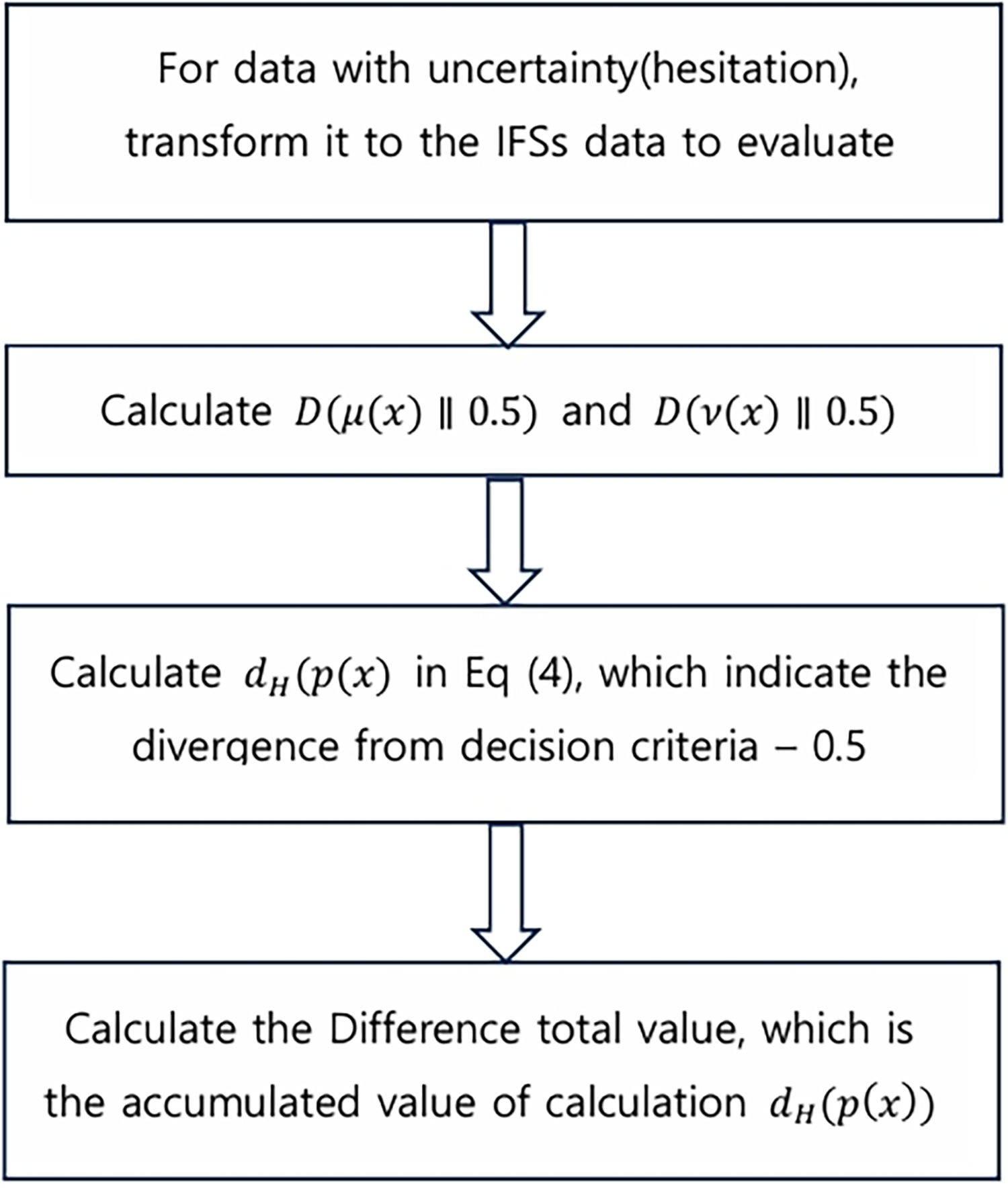
Figure 5: Accumulate hesitation calculation

Temporal data can be updated with sequential probability values pk(x), which are the instantaneous values of dH(p(x)). Then the accumulated values indicate total hesitation values to the decision criterion–0.5. The results are illustrated using a Korean congressional election census poll and are discussed in the next section.

4  Illustrative Example

To summarize, there is a great relationship between Western rhetoric and English writing, rhetoric is not only the use of rhetoric. However, the use of figures of speech can provide some very useful writing skills for English writing. Rhetoric, as a whole, is an art of persuasion. In the process of using various rhetorical devices to write, English writers should pay attention to strengthening their understanding of rhetoric itself and the knowledge covered within it, and combine the rhetorical perspective to improve their ability to use rhetorical devices such as contrastive, exaggeration and so on. In this section, KL divergence is applied to analyze election results, specifically focusing on the Korean congressional elections. This example interprets election information through KL divergence, examining two cases of electoral competition to illustrate its application.

4.1 Korean National Assembly Election

KL-divergence calculation, applied to support and hesitation metrics in a model of Korean congressional election, is derived from information theory principles [21]. The 22nd Korean congressional election took place on 10 April 2024. There are 300 seats contested: 254 for district representatives and 46 for proportional representation. The district map in Korea is shown in Fig. 6.

Figure 6: Korean delegates districts

Election prediction measures have been stated by Buchanan, even though there was existing research [28]. It was pointed out that the poll proportion predicts the winner correctly. The South Korean National Assembly elections have undergone significant transformations over the years, reflecting shifts in political ideology, electoral processes, and voter behavior. Historically, these elections have been characterized by intense competition between the two dominant parties: the progressive and conservative blocs. Since the democratization of South Korea in 1987, these elections have played a critical role in shaping national policies and governance. The 21st congressional election, held in 2020, was particularly noteworthy as it witnessed a landslide victory for the progressive party, securing 163 out of 300 total seats, while the conservative party managed to secure only 84. This outcome significantly influenced subsequent policy directions, including economic reforms, diplomatic strategies, and responses to social issues.

The 2024 election cycle presented a different landscape, with increased voter volatility and fluctuating approval ratings for both major parties. In the months leading up to the election, polling data indicated a narrowing gap between candidates, reflecting a more competitive political climate. The role of undecided voters was particularly significant in this cycle, with their shifting preferences impacting both major parties’ campaign strategies. Moreover, the influence of external factors, such as economic downturns, diplomatic challenges, and domestic social movements, further shaped voter sentiment. Understanding these historical trends and their implications provides crucial context for analyzing hesitation patterns and decision-making dynamics in the electoral process.

For the 2024 election, these two major parties are again the main contenders. Over the past two months leading up to the election, their respective support levels have varied, as documented by candidate polling data collected from the National Election Commission (NEC) [23]. Support trends for each candidate across all districts are available, representing major and sometimes minor candidates based on relevance.

Considering the support histories for two leading candidates, Figs. 7 and 8 examine the support, dissent, and abstention percentages for the 10 April 2024 voting outcome. Fig. 7 shows that two candidates are decisive; candidate A overwhelmingly beats B over the polling period and resulting in a swell. We can recognize that the undecided class becomes shorter in the final. Candidate A starts with 44% support and eventually garners 51.47% support. Whereas, Fig. 8 depicts two competitive candidates, with fluctuating results on the final voting day. In this case, the result is not easily predictable with any measure. In this regard, KL-divergence calculation, applied to support and hesitation metrics in a model of Korean congressional election, is derived from information theory Two candidates showed a continual gap throughout the polling period. From the figure, support, dissent, and abstention are considered membership values for IFSs, which is also included in one of the examples in existing research [29].

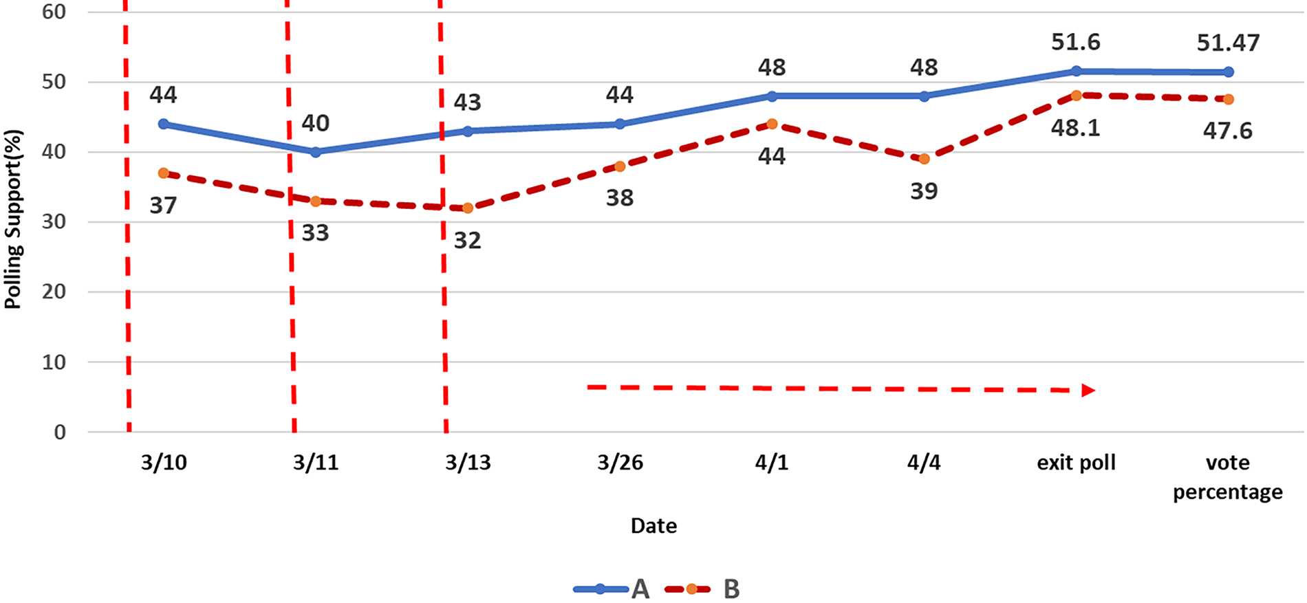
Figure 7: PollTrends in District 1 from 10th March to vote result in 10 April (%)

Figure 8: PollTrends in District 3 from 13th March to vote result in 10 April (%)

Each percentage is represented by the membership values: membership value μ(x) represents support. For example, candidate A’s supportive 51.47% corresponds to μA(x)=0.5147, whereas μB(x)=0.47 for candidate B. The non-membership value ν(x) represents dissent. For candidate A, νA(x)=0.47, meanwhile νB(x)=0.5147. Hesitation is represented by abstention, where both πA(x)=0.0093 and πB(x)=0.0093 are assigned to process IFSs.

Another competitive case is illustrated in Fig. 8. Candidate A starts with 47.1% and eventually garners 45.98% support. Two candidates showed up and down by the voting date–10 April. Each percentage is represented by the membership values: A’s supportive to μA(x)=0.4598, whereas μB(x)=0.5401 for candidate B finally. The non-membership value ν(x) represents as the same ways; dissent. νA(x)=0.05401, meanwhile νB(x)=0.4598. Hesitation is represented by abstention, where both πA(x)=0.00001 and πB(x)=0.00001.

Fig. 7 highlights a decisive trend, while Fig. 8 illustrates a close contest, prompting a focus on calculating ds(pk(x)) in Fig. 8, then the calculation results of candidates A and B of Fig. 8 are illustrated in the tables of the next subsection together with the difference and the summation of supportive history. The election result is that candidate B wins. But the process was competitive and not easy to predict. The following insights summarize the trends observed;

•   Candidate B’s support trend was relatively stable, with minimal fluctuation.

•   Exit polls and final vote percentages represent the actual election outcome and are not included in the information analysis.

Figs. 7 and 8 illustrate sequential data, Fig. 7 displays temporal data updates that influence current and future outcomes.

A:0.44−0.4−0.43−0.44−0.48−0.48−0.516−0.5147

Decisions are made through iterative data sequences using prior and posterior distributions. Each update informs the next decision. Given the information I, the prior distribution p(x), can be updated to a posterior p(x|I) when new evidence y emerges, leveraging the KL divergence. Applying the KL-divergence, we assess the utility of new information by updating the conditional distribution to determine if it holds value. Using Eqs. (8) and (9), we calculate the proposed conditional KL-divergence based on election pool data. Here, p(x|y,I), p(x,I) reflect the winning probability based on median poll values over a defined census period:

p(x=win|y1=13th Mar.,…,yn=4th Apr.)p(x=win|y1=13th Mar.,…,yn−1=1st Apr.)

where p(x,I) is assigned by the winning probability with the mid values of the poll between two candidates over the census duration. Specifically,

I=47.1+41.42,…,48+432.

For instance, supportiveness can range between 44.25% and 45.5%, indicating an election could be won at this support level. However, an election-win threshold of 50% must still be considered, although it is not directly addressed here.

4.2 Recognition Comparison

The results of two recognition calculations are illustrated. By calculating hesitation in each candidate’s support using Eq. (6)—ds(pk(x))—together with its difference and accumulated hesitation are illustrated in Tables 1 and 2. as the difference total. While both census results are presented, only one election poll is decisive and predictive, as shown in Fig. 7. Conversely, Fig. 8 highlights a more competitive polling history. Candidate B exhibits stability here, whereas Candidate A shows continuous, albeit fluctuating, growth. Specific census data on 1 and 4 of April indicate variability, complicating predictive efforts. Ultimately, candidate B won, indicating significant support. To support this observation, we also examined simple statistical indicators such as the variance of support ratios across the polling period, which was lower for Candidate B than for Candidate A, indicating greater stability and consistency in voter preference. Notably, only when pk(x)>0.5 does ds(pk(x)) produce positive values, and Candidate A’s hesitation fluctuates, as shown by the alternated signs in Table 1.

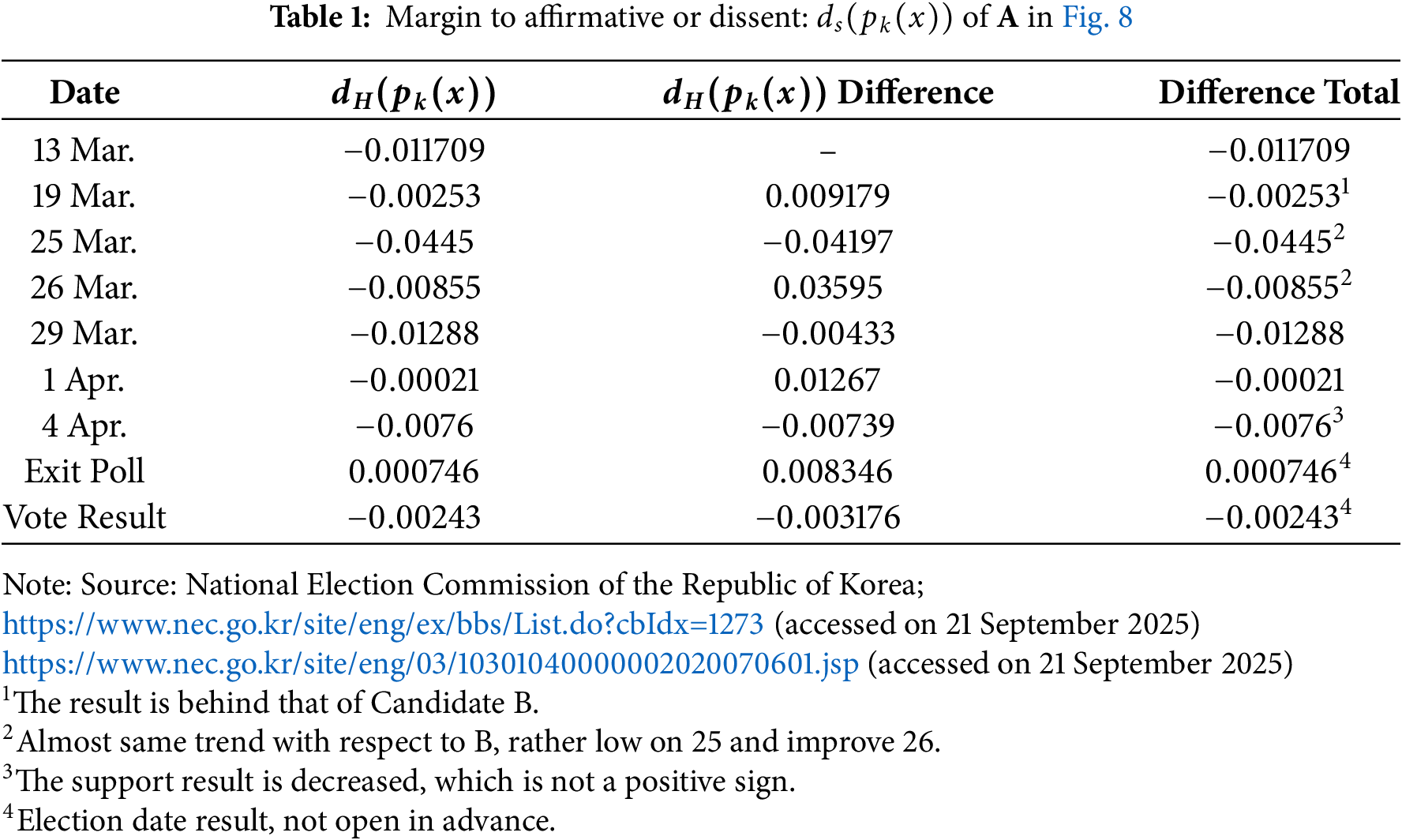
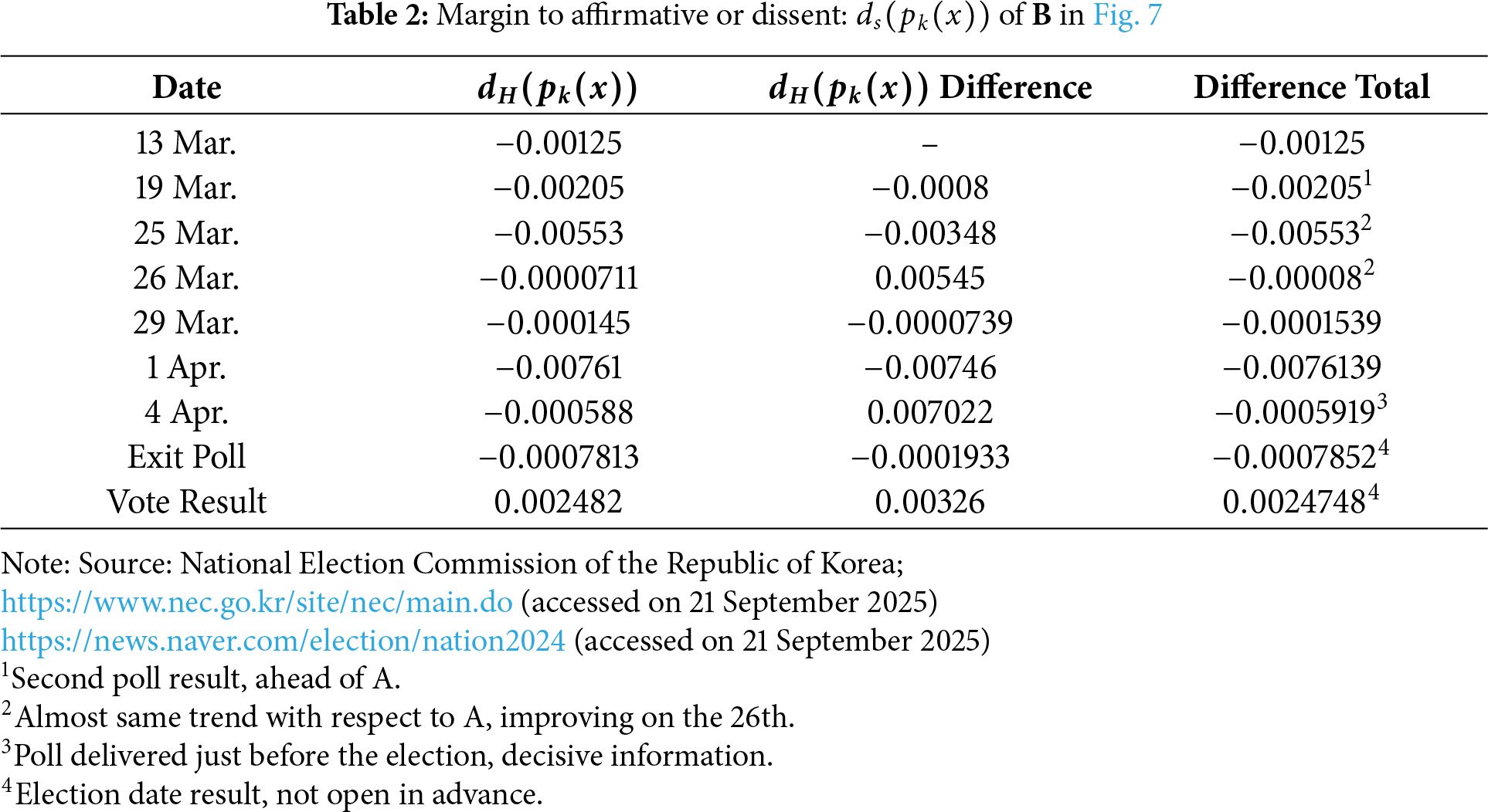
Conversely, Table 2 shows a continuous reduction in hesitation for Candidate B, suggesting sustained support. A lower difference total often implies consistent support, and ds(pk(x)) calculations approach zero, reflecting Candidate B’s support nearing 50%. It is essential to clarify that “Exit poll” and “Vote result” represent election outcomes that are not part of the preliminary information.

Next, the conditional KL divergence calculation is conducted based on the updated information. Using Eq. (9), the likelihood function is represented as p(y|x,I) and is structured linearly, as demonstrated by prior findings [21]. Poll data from District 3, as shown in Fig. 8, are used to calculate the conditional KL divergence for Candidate A, while the results for Candidate B are also noted.

0.414log20.4140.4425+0.459log20.4590.461+0.34log20.340.39+0.426log20.4260.4595+0.41log20.410.45+0.488log20.4880.4595+0.43log20.430.455

Candidate B also shows the following values:

0.471log20.4710.4425+0.463log20.4630.461+0.44log20.440.39+0.493log20.4930.4595+0.49log20.490.45+0.431log20.4310.4595+0.48log20.480.455Candidate A:−0.2042,Candidate B:0.2280.

From these results, Candidate A’s likelihood of winning appears relatively high but falls below the winning criterion, which aligns with the margin insufficiency discussed in Section 3.2. Conversely, Candidate B’s likelihood exceeds the sufficiency margin of 0.5—indicating a high probability of winning, consistent with findings in Tables 1 and 2. The supportive data for both candidates also reflect a degree of hesitation, as revealed in the calculations.

4.3 Discussion

The hesitation metric incorporates KL divergence calculated by comparing values supportive or opposed to a threshold of 0.5, expressed as D(p(x)‖0.5), where p(x) represents affirmative or opposing views, as addressed by Eq. (5).

dH=d(p(x))−d(q(x))(10)

p(x) deviates further from decision boundary—generally set at 0.5—than q(x). This calculation reflects the current status, underscoring the need for ongoing data analysis to accurately assess trends for each candidate. The election poll example shows the pivotal role of KL divergence in predicting likely outcomes and supporting decision-making. However, predicting abrupt trend shifts, such as those illustrated in Fig. 8, remains challenging because of unpredictable external factors. Then, the proposed method facilitates a meaningful and accurate conclusion; rather than relying on instantaneous KL divergence values. These are accumulated data yielding lower variance, reflecting reduced hesitation. According to these results, excluding exit poll and final voting outcomes, Candidate A records a value of −0.0076 while Candidate B records −0.0005919: it is a natural result that Candidate B is closer to winning. Although both values are close to 0.5, indicating similar hesitation, Candidate B’s value trends closer to the mid-point. Although the calculations depicted in Fig. 7 were not detailed here, their results would be definitive. In the conditional KL divergence, we simplify the calculation as follows: p(x|y,I) represents the supportive factors, and p(x|I) denotes the winning rate in Eq. (8). Calculations updated as of April 4 indicate that candidate B shows a relatively high value, with A at −0.2042 and B at 0.2280. These values suggest that both candidates approach the winning criterion, yet candidate B holds a slight advantage by KL divergence standards. Intriguingly, despite potential voter confusion, the results align consistently across calculation methods.

In future research, we aim to explore approaches incorporating information weighting akin to a Markovian approach. Applying IFS data in KL-divergence calculations simplifies the process by mapping membership functions to affirmative or dissenting categories. The proposed KL divergence approach has significant potential for enhancement, particularly in refining the winning distribution and dynamically integrating poll data with additional variables. Additionally, analyzing the middle-class voter shift is interesting, as this demographic often critically influences election outcomes. The result is summarized as follows;

•   The example presents precise IFS data, including affirmative and dissenting information, allowing for considering hesitation values.

•   Although hesitation information is calculated using the proposed methods, its behavior is somewhat unclear.

•   Result from Table 2 is chosen from one of the competitive election districts. The difference total should be positive if candidate B wins. However, we observe a negative value trend, rather than an increasing one.

•   Most of the uncovered results are basically decisive, and the calculations are not included.

The implications of hesitation analysis in electoral decision-making extend beyond mathematical modeling and probability calculations. In a democratic society, elections serve as the primary mechanism for expressing public will, and understanding voter hesitation can provide insights into broader socio-political trends. The presence of hesitation among voters reflects uncertainty and the complex interplay of political preferences, media influence, and economic considerations. By quantifying hesitation using Kullback-Leibler (KL) divergence, this study contributes to a deeper understanding of electoral behavior, offering valuable perspectives for policymakers, political analysts, and strategists. From a social standpoint, analyzing hesitation trends can help identify demographic segments that are more susceptible to shifts in political allegiance, thereby guiding targeted voter outreach efforts. Furthermore, this research highlights the importance of information dissemination in reducing voter uncertainty, ensuring that electoral decisions are based on well-informed judgments rather than momentary influences. Politically, hesitation analysis can aid in refining predictive models for election outcomes, improving strategic decision-making in campaign management. In the broader scope, this study underscores the role of information theory in political science, bridging the gap between computational methodologies and electoral studies to enhance the accuracy and reliability of decision-making frameworks. This hesitation-based KL divergence framework is not intended to replace standard predictive models, such as logistic regression or decision trees, but rather to complement them by quantifying the unique role of hesitation and uncertainty in decision-making scenarios.

5  Conclusions

This study proposes a method to calculate hesitation values by leveraging the KL divergence. Since hesitation originates from IFSs, it requires predefined membership and non-membership values. Here, hesitation is calculated by examining the affirmative and dissent degrees, interpreted as membership and non-membership structures within IFSs. Consequently, KL-divergence is modified using Bayes’ theorem in conjunction with concepts from information theory, such as entropy and cross-entropy. Additionally, conditional KL divergence is proposed to address decision-making challenges. To optimize this approach, preference values for attributes and reference values for criteria are expressed as IFSs. These values contribute to calculating KL divergence between attributes, influencing decision accuracy. The two KL-divergence metrics proposed have distinct implications for decision-making: the first evaluates proximity to criteria based on given IFSs. In contrast, the second assesses hesitation in temporal data applications. Typically, cumulative data significantly influence decision outcomes; calculations indicate that fluctuations in supportive data intensify hesitation levels. The results underscore the importance of deriving attribute values from existing data or through further development. The demonstrated example—examining election data from Korean Congressional members—highlights the importance of incorporating updated information in decision-making processes. With the calculation, we can recognize the voters hesitation trend whether they support or not. The analysis shows that two consistent decision-making approaches yield reliable results: hesitation accumulation and conditional KL divergence. The research output is expected to be a useful foundation for decision problems in future research. Although the methodology was demonstrated on electoral data, its formulation is general and can be extended to diverse domains such as medical diagnostics, financial risk assessment, and social decision-making processes where hesitation is critical.

Acknowledgement: New Uzbekistan University, Uzbekistan, Ministry of Education of the Republic of Korea and Kookmin University, Republic of Korea.

Funding Statement: Uzbekistan to China International Science and Technology Innovation Cooperation: IL-8724053120-R11 and National Research Foundation of Korea: NRF-2025S1A5A2A01011466.

Author Contributions: Conceptualization, Sanghyuk Lee; methodology, Sanghyuk Lee; software, Eunmi Lee; validation, Eunmi Lee; formal analysis, Sanghyuk Lee, Eunmi Lee; investigation, Eunmi Lee; resources, Eunmi Lee; data curation, Sanghyuk Lee, Eunmi Lee; writing—original draft preparation, Sanghyuk Lee, Eunmi Lee; writing—review and editing, Sanghyuk Lee, Eunmi Lee; visualization, Eunmi Lee; supervision, Sanghyuk Lee. All authors reviewed the results and approved the final version of the manuscript.

Availability of Data and Materials: https://www.nec.go.kr/site/eng/ex/bbs/List.do?cbIdx=1273, https://www.nec.go.kr/site/eng/03/10301040000002020070601.jsp (accessed on 20 August 2025).

Ethics Approval: Not applicable.

Conflicts of Interest: The authors declare no conflicts of interest to report regarding the present study.

References

1. Xiao F, Wen J, Pedrycz W. Generalized divergence-based decision making method with an application to pattern recognition. IEEE Trans Knowl Data Eng. 2022;35(7):6941–56. doi:10.1109/TKDE.2022.3177896. [Google Scholar] [CrossRef]

2. Guo J, Guo F, Ma Z, Huang X. Multi-criteria decision making framework for large-scale rooftop photovoltaic project site selection based on intuitionistic fuzzy sets. Appl Soft Comput. 2012;102:107098. doi:10.1016/j.asoc.2021.107098. [Google Scholar] [CrossRef]

3. Gohain B, Chutia R, Dutta P, Gogoi S. Two new similarity measures for intuitionistic fuzzy sets and its various applications. Int J Intell Syst. 2022;37(9):5557–96. doi:10.1002/int.22802. [Google Scholar] [CrossRef]

4. Taherdoost H, Madanchain M. Multi-criteria decision making (MCDM) methods and concepts. Encyclopedia. 2023;1(1):77–87. doi:10.3390/encyclopedia3010006. [Google Scholar] [CrossRef]

5. Ishizaka A, Nemery P. Multi-criteria decision analysis: methods and software. Chichester, West Sussex, UK: Wiley; 2013. 81 p. [Google Scholar]

6. Hong DH, Choi CH. Multicriteria fuzzy decision-making problems based on vague set theory. Fuzzy Sets Syst. 2000;114(1):103–13. doi:10.1016/S0165-0114(98)00271-1. [Google Scholar] [CrossRef]

7. Zhu Z, Locatello F, Cevher V. Sample complexity bounds for score-matching: causal discovery and generative modeling. In: NeurIPS 2023 Conference; 2023 Dec 10–16; New Orleans, LA, USA. 1 p. doi:10.48550/arXiv.2310.18123. [Google Scholar] [CrossRef]

8. Pelissari R, Oliveira MC, Abackerli AJ, Ben-Amor S, Assumpcao MRP. Techniques to model uncertain input data of multi-criteria decision-making problems: a literature review. Int Trans Oper Res. 2021;28(2):523–59. doi:10.1111/itor.12598. [Google Scholar] [CrossRef]

9. Yatsalo B, Korobov A. Different approaches to fuzzy extension of an MCDA method and their comparison. In: Intelligent and Fuzzy Techniques: Smart and Innovative Solutions: Proceedings of the INFUS 2020 Conference; 2020 Jul 21–23; Istanbul, Turkey: Springer; 2021. p. 709–17. [Google Scholar]

10. Kizielewicz B, Paradowski B, Wieckoswki J, Salabun W. Towards the identification of MARCOS models based on intuitionistic fuzzy score functions. In: 17th Conference on Computer Science and Intelligence Systems (FedCSIS); 2022 Sep 4–7; Sophia, Bulgaria: IEEE. p. 789–98. [Google Scholar]

11. Atanassov KT. Intuitionistic fuzzy sets. Fuzzy Sets Syst. 1986;20(1):87–96. doi:10.1016/S0165-0114(86)80034-3. [Google Scholar] [CrossRef]

12. Mahanta J, Panda S. A novel distance measure for intuitionistic fuzzy sets with diverse applications. Int J Intell Syst. 2021;36(2):615–27. doi:10.1002/int.22312. [Google Scholar] [CrossRef]

13. Patel A, Kumar N, Mahanta J. A 3D distance measure for intuitionistic fuzzy sets and its application in pattern recognition and decision-making problems. New Math Nat Comput. 2023;19(2):447–72. doi:10.1142/S1793005723500163. [Google Scholar] [CrossRef]

14. Zadeh LA. Toward a theory of fuzzy information granulation and its centrality in human reasoning and fuzzy logic. Fuzzy Sets Syst. 1997;90(2):111–27. doi:10.1016/s0165-0114(97)00077-8. [Google Scholar] [CrossRef]

15. Bargiela A, Pedrycz W. Toward a theory of granular computing for human-centered information processing. IEEE Trans Fuzzy Syst. 2008;16(2):320–30. doi:10.1109/TFUZZ.2007.905912. [Google Scholar] [CrossRef]

16. Mahmood MA, Almuayqil S, Alsalem KO. A granular computing classifier for human activity with smartphones. Appl Sci. 2023;13(2):1175. doi:10.3390/app13021175. [Google Scholar] [CrossRef]

17. Li J, Mei C, Xu W, Qian Y. Concept learning via granular computing: a cognitive viewpoint. Inf Sci. 2015;298(2):447–67. doi:10.1016/j.ins.2014.12.010. [Google Scholar] [PubMed] [CrossRef]

18. Yao JT, Yao Y, Ciucci D, Huang K. Granular computing and three-way decisions for cognitive analytics. Cognit Comput. 2022;14(6):1801–4. doi:10.1007/s12559-022-10028-0. [Google Scholar] [CrossRef]

19. Kullback S, Leibler RA. Information and Sufficiency. Ann Mathem Statist. 1951;22(1):79–86. doi:10.1214/aoms/1177729694. [Google Scholar] [CrossRef]

20. Seghouane AK, Amari SI. The AIC criterion and symmetrizing the kullback-leibler divergence. IEEE Trans Neural Netw. 2007;18(1):97–106. doi:10.1109/TNN.2006.882813. [Google Scholar] [PubMed] [CrossRef]

21. Cover TM, Thomas JA. Elements of information theory. Hoboken, NJ, USA: Wiley-Interscience; 2006. 19 p. [Google Scholar]

22. Panda K, Dabhi D, Mochi P, Rajput V. Levy enhanced cross entropy-based optimized training of feedforward Neural Networks. Eng Technol Appl Sci Res. 2022;12(5):9196–202. doi:10.48084/etasr.5190. [Google Scholar] [CrossRef]

23. National Election Commission of the Republic of Korea; 2024. [cited 2025 Sep 21]. Available from: http://www.nec.go.kr/site/nec/main.dohttps://www.news.naver.com/election/nation202. [Google Scholar]

24. Conforti G, Durmus A, Silveri MG. KL convergence guarantees for score diffusion models under minimal data assumptions. arXiv:2308.12240. 2024. doi:10.48550/arxiv.2308.12240. [Google Scholar] [CrossRef]

25. Khan SZ, Rahim M, Widyan AM, Almutairi A, Almutire NSE, Khalifa HAE. Development of AHP-based divergence distance measure between p, q, r—spherical fuzzy sets with applications in multi-criteria decision making. Comput Model Eng Sci. 2025;143(2):2185–211. doi:10.32604/cmes.2025.063929. [Google Scholar] [CrossRef]

26. Li Y, Rahim M, Khan F, Khalifa H. A TODIM-based cubic quasirung orthopair fuzzy MCGDM model for evaluating 5G network providers using Minkowski distance and entropy measures. Expert Syst Appl. 2026;296 A(15):128908. doi:10.1016/j.eswa.2025.128908. [Google Scholar] [CrossRef]

27. Lee S, Lee E. Score function design for decision making using conditional kullback-leibler divergence. In: IEEE International Conference on Artificial Intelligence in Engineering and Technology; 2024 Aug 26–28; Kota Kinabalu, Malaysia. doi:10.1109/IICAIET62352.2024.10730591. [Google Scholar] [CrossRef]

28. Buchanan W. Election predictions: an empirical assessment. Public Opinion. 1986;50(2):222–7. doi:10.1086/268976. [Google Scholar] [CrossRef]

29. Lee S, Ravshanovich KA, Pedrycz W. Relation on hesitation in intuitionistic fuzzy sets and decision making. In: IEEE EUROCON—International Conference on Smart Technologies; 2025 Jun 4–6; Gdyniz, Poland. doi:10.1109/EUROCON64445.2025.11073281. [Google Scholar] [CrossRef]