Classification Method of Lower Limbs Motor Imagery Based on Functional Connectivity and Graph Convolutional Network

1  Introduction

Brain-computer interface (BCI) can measure brain activity related to intention and transmit brain signals to external devices. Motor imagery (MI), the most common non-invasive BCI paradigm, allows users to imagine limb movements and actively control the system. MI-BCI helps patients with motor disorders live better by bypassing injured neuromuscular pathways. However, most MI-BCI studies are limited to upper limb MI [1–3], such as left hand, right hand, and elbow. As for lower limb MI, the sensory-motor cortex regions activated during the imagination of the left and right lower limbs limb are anatomically very close [4], and the activation is located at a deeper location (interhemispheric fissure cistern) [5], leading to a low signal-to-noise ratio (SNR) and difficulty in producing distinguishable features. Such issues do not exist with upper limb MIs. Therefore, MI for both left and right lower limbs is typically treated as a single task and classified alongside other MI tasks. This is unfavorable for developing a BCI system for lower limb movement. Although classifying lower limb MI is complex and challenging, the development of BCI applications related to lower limb MI has great potential [6].

The brain network mainly includes two types: structural network and functional network [7]. A structural network is composed of electrical or chemical connections between neuronal synapses, typically showcasing the brain’s fine structure through anatomical and imaging methods. Functional networks are estimated using statistical models based on functional magnetic resonance imaging (fMRI) or EEG to reveal differences in brain network structure in neurological disorders. Since functional connectivity (FC) can effectively describe the features of brain activity patterns across varied brain regions, it is of great significance for studying brain networks and their mechanisms.

Although fMRI has superior spatial resolution to EEG, the lower spatio-temporal resolution, high cost, and limited physical space are not conducive to the large-scale application of real-time brain-computer interface (BCI) systems. Therefore, an increasing number of researchers have begun to study FC based on EEG. Due to the discrete nature of EEG channels in space, FC is located in non-Euclidean space. If each channel is considered a node, there will be a significant amount of cross-node interaction. Compared to traditional convolutional neural networks, graph convolutional networks (GCN) can mine cross-node topological features in graphs and more effectively handle data with spatiotemporal interactions. Although GCN has attracted a large number of researchers’ attention, lower limb MI classification methods based on GCN and utilizing FC features have yet to be explored.

This study proposes a left and right foot MI classification method that combines FC features with GCN. Specifically, we first calculate the functional connectivity of EEG signals based on PLV. Then, we use the obtained adjacency matrix and the original EEG signals as inputs to the temporal-spatial GCN (TSGCN) for classification. Compared with the conventional ST-GCN [8], our TSGCN fully leverages the functional connectivity provided by PLV, thereby effectively integrating inter-channel correlations in EEG signals and capitalizing on their physiological characteristics.

The main contributions of this study are as follows. 1) A method combining FC features and GCN was proposed to classify left and right foot MI, achieving higher classification performance. 2) In response to the characteristics of EEG data, the structure of GCN has been improved, and a new TSGCN has been proposed, effectively utilizing the features of time and space domains. 3) Analyzed the graph-theoretic characteristics of left and right foot MI, revealed its internal network mechanism, and laid the foundation for future research.

2  Related Work

2.1 Lower Limb MI Classification Methods

Numerous studies have been conducted on classifying upper limb MI, but little attention has been paid to lower limb MI. Gu et al. [9] used sparse multi-logistic regression (SMLR) as a feature selector, and then proceeded to select support vector machines (SVM) as the classification model, reaching an average classification accuracy of 67.13%. Tariq et al. [10] used the filter bank typical spatial pattern (FBCSP) to refine the frequency bandwidth selection, and then obtained the mean value of classification accuracy of 70.28% through linear discriminant analysis (LDA). With the rapid development of deep learning, methods based on convolutional neural networks have achieved higher classification performance. Lu et al. [11] used the short-time Fourier transform (STFT) to convert the signal into a time spectrum and then constructed a practical convolutional neural network (pCNN), achieving an average classification accuracy of 72.13%. Recently, Sun et al. [12] proposed two classification methods based on Riemannian clustering: margin based Riemannian clusters (MBRC) and statistics based Riemannian clusters (SBRC). These two methods achieved average classification accuracies of 71.29% and 73.12%, respectively.

2.2 Functional Connectivity

To effectively classify left and right foot MI, it is necessary to construct an adjacency matrix containing topological relationships between different EEG channels as a critical input for GCN. Functional connectivity is frequently used in cognitive neuroscience, such as emotion recognition [13], mild cognitive impairment [14], and severe depression [15]. Some traditional measures include Pearson correlation [16], tanh nonlinearity [17], mean correlation coefficient [18], and covariance [19], which cannot fully represent complex brain connections. Therefore, researchers have developed many methods to measure FC, mainly divided into three categories: time-domain, frequency-domain, and time-frequency domain. The time-domain methods include phase lag index (PLI) [20] and phase locking value (PLV) [21], while the frequency-domain methods include imaginary part of coherence (IPC) [22] and amplitude squared coherence (MSC) [23], as well as wavelet coherence (WC) that combines time-domain and frequency-domain [24]. These metrics can better describe the degree of synchronization in different brain regions and the changes resulting from their interactions. Some studies have applied metrics such as PLV, mutual information (MI), and transfer entropy (TE) to calculate the functional connectivity of hand, foot, and tongue MI [25–27].

2.3 Graph Convolutional Network

In recent years, GCN has demonstrated its ability to model multi-channel signals in non-Euclidean spaces. Therefore, some researchers have begun to attempt to apply GCN to EEG-based EEG signal classification tasks. Shi et al. [28] proposed a Tuned Heuristic Fusion Graph Convolutional Network (THFGCN) for limb movement prediction in rehabilitation scenarios. The validation experiments conducted on the PhysioNet and LLM-BCImotion datasets show that the accuracy of the THFGCN method for the same individual cases is 88.4% and 82.82%, while for cross-individual cases, it is 65.93% and 60.56%. Demir et al. [29] developed multiple GCN models, which achieved higher performance than CNN on public datasets based on P300 and RSVP paradigms. Xiao et al. [30] proposed a spatiotemporal graph convolutional network based on the pLSTM self-supervised module and attention-guided drop mechanism, which achieved significant improvements on the KIMORE dataset. Sun et al. [31] introduced an adaptive spatio-temporal convolutional network for the 2-class classification task of lower limb MI. This method dynamically integrates channel information and fully utilizes spatio-temporal information, surpassing existing SOTA methods in terms of classification accuracy and robustness. Although GCN has received considerable attention, the GCN model applied to left and right foot MI classification has yet to be fully studied.

3  Method

As illustrated in Fig. 1, the preprocessed EEG signals were further processed using PLV to construct the adjacency matrix representing the functional connectivity strength among the selected nine channels. This matrix was then fed into the proposed temporal-spatial graph convolutional network (TSGCN) for feature extraction. The TSGCN is composed of two spatio-temporal convolutional blocks, each consisting of two temporal convolution layers and one spatial graph convolution layer. Finally, classification was achieved through a fully connected dense layer. Since we use PLV to construct the GCN, the adjacency relationships in EEG signals are integrated more effectively. In addition, adding a temporal convolution block alongside the GCN enables the network to fully exploit the high temporal resolution of EEG signals.

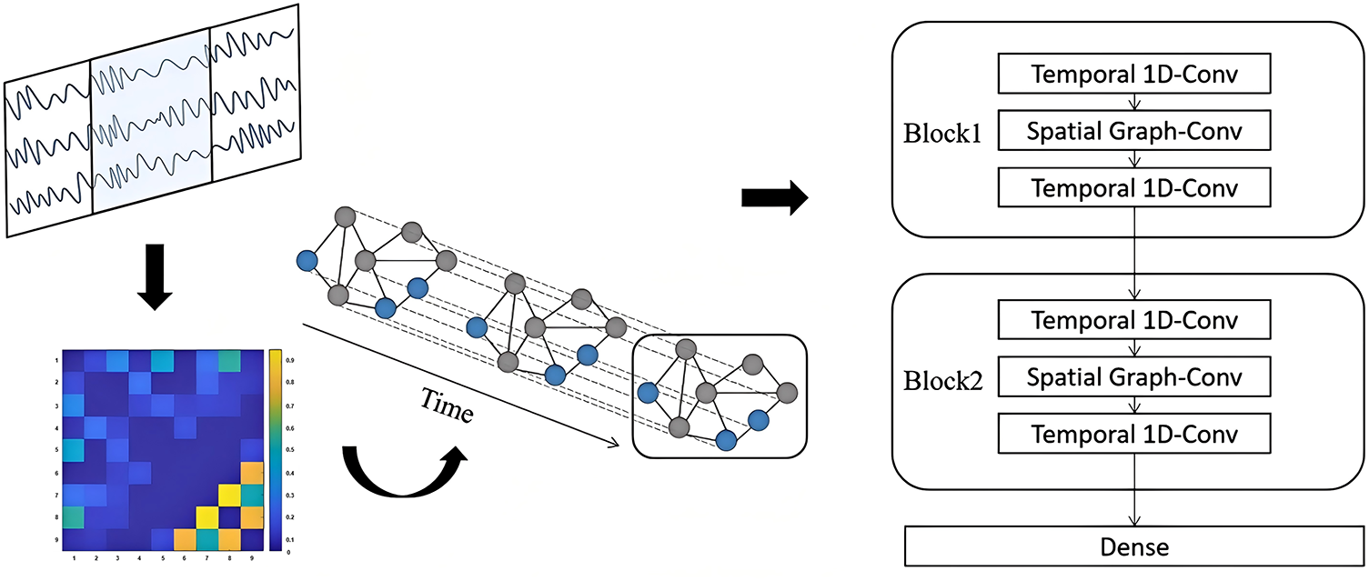
Figure 1: The overview of the method. The TSGCN is composed of two spatio-temporal convolutional blocks, each consisting of two temporal convolution layers and one spatial graph convolution layer. Finally, classification was achieved through a fully connected dense layer

3.1 PLV

PLV is a statistical measure used to study phase synchronization among signals. During this research, PLV is used to estimate the instantaneous phase relationship among each EEG channel. Since the Hilbert transform performs better in calculating the instantaneous phase of narrowband signals, the original signal needs to be filtered and the desired frequency bandwidth selected before calculating PLV. PLV is defined as follows:

PLV(time,ω)=1N|∑n=1Nexp(jΔφn(time,ω))|(1)

time denotes the instantaneous time, ω denotes the selected frequency bandwidth, N denotes the count of trials, and Δφn denotes the instantaneous phase difference among different channels.

Then, determine the elements Wij of the adjacency matrix W according to PLV. The calculation is as follows:

Wij={PLVij,ifPLVij≥T0,otherwise(2)

Among them, T is a fixed threshold, PLVij represents the functional connection strength between node i and node j.

3.2 Temporal-Spatial Convolutional Network

In traditional convolutional networks, the convolution operation employs filters with shared parameters to extract spatial features by computing weighted sums between a central pixel and its neighbors. However, this operation is limited to data with regular Euclidean structures. To address non-Euclidean and irregular domains such as brain networks, the graph convolution method has been proposed, which generalizes the convolution operation to graph-structured data.

Spatio-temporal convolution is based on ordinary convolution in the time dimension, with graph convolution added in the spatial dimension according to the topological structure of the data. Compared with ordinary convolution, which can only extract spatial features, spatio-temporal convolution can also extract additional temporal features. This research uses the characteristics of graph convolution to obtain information from neighboring nodes in the brain network to extract spatial features. Graph convolution is specifically defined as follows:

gθ(L)x=gθ(UΛLT)x=Lgθ(Λ)UTx(3)

Among them, gθ acts as a filter used to reduce computational complexity. It could be approximated by truncating Chebyshev polynomials, as detailed in [32].

gθ(Λ)=∑p=0k−1θpTp(Λ~)(4)

We use a one-dimensional convolution layer to obtain temporal features. The second convolution layer can be defined as:

χh(r)=Φ∗(ReLU(gθ∗Gχ^h(r−1)))(5)

Among them, Φ is convolution kernel parameter, ∗ is the convolution operations, and ReLU is the activation functions.

The core reason why GCN works effectively lies in its special form of Laplacian smoothing, but it also brings potential issues of over smoothing [33]. According to previous research, GCN is typically set to two layers [34–36]. Therefore, the model proposed in this article also uses two GCN layers. Specifically, the TSGCN proposed in this study is composed of two temporal-spatial convolutional blocks stacked together, each block containing two temporal convolutional layers and one spatial graph convolutional layer. The kernel size for each temporal convolution is 9×1, and the kernel size for each spatial convolution is 1×1. Each spatiotemporal convolutional block has undergone Layer Normalization (LN) and ReLU to prevent overfitting. Apply dropout with a probability of 0.5 after the two blocks. The fully connected layer is used to classify the extracted features. The overall framework of the proposed method is shown in Fig. 1.

4  Experiment

Due to the current lack of publicly available lower limb MI datasets for evaluation, existing research is based on internal laboratory datasets. Therefore, this study designed a data collection experiment and compared the proposed method with existing methods on an in-house dataset.

4.1 Dataset Description

This study recruited 10 healthy participants, including 6 males and 4 females, with an average age of 24.7 years old. All participants had no history of neuromuscular diseases or color vision defects. Before the experiment, we explained the experimental process, and the participants signed an informed consent form. EEG was recorded from 10 participants, where the authors work collaborated with Zhejiang Hospital, China. The Ethics Committee of the Zhejiang Hospital approved the study (Approval No. 2025-C-095).

The participants sat in a comfortable chair and looked at the monitor from a distance of approximately 50cm. The participants wore a 64-channel EEG cap and accurately located it according to the international 10–20 system. All channels are sampled at a frequency of 1000 Hz.

The experimental paradigm is illustrated in Fig. 2. Each trial lasts for 8 s. The monitor displays a gray cross in the first 2 s, indicating that the subjects can take a break. Subsequently, the gray cross lights up, indicating that the subjects are ready and the experiment is about to begin. A random sequence of images of left or right footprints appeared on the 3–8 s display, and as a response to the prompt, the subjects were required to complete the corresponding MI task, which involved imagining kicking their left or right foot rapidly. The experiment consists of six sessions, each consisting of 20 trials (10 with the left foot and 10 with right foot). Participants can rest for 5 min between each round of experiments to prevent fatigue. Therefore, for each participant, a 36-min experiment was conducted, and a total of 120 trials were completed. The dataset contains a total of 1200 trials.

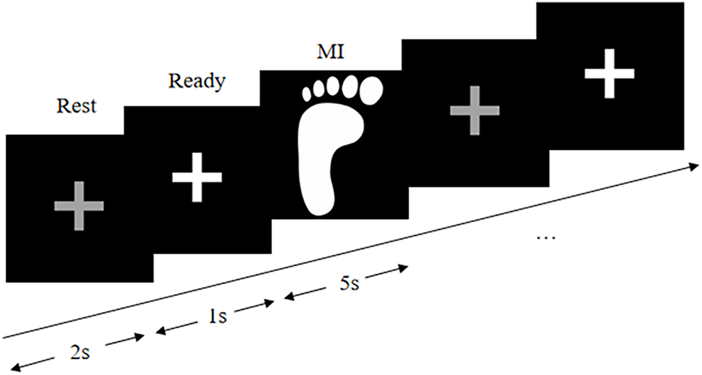
Figure 2: Left foot experimental paradigm of in-house dataset

4.2 Preprocessing and Training

Similarly processing upper limb MI data, we preprocess the original signal to improve SNR before extracting features from lower limb MI data. Firstly, the EEG signal is downsampled to 250 Hz. Then, 50 Hz power frequency filtering, 0.5 Hz high pass filtering, and 45 Hz low pass filtering were performed. Subsequently, an average re-reference is performed to reduce interference from various channel instability. Then, independent component analysis (ICA) was conducted to eliminate noise. Finally, based on the research of Liu et al. [37], this study selected nine electrodes centered around Cz (C3, C4, Cz, F3, F4, Fz, P3, P4, and Pz).

We train the model using stochastic gradient descent with an initial learning rate of 0.01. The learning rate is reduced by a factor of 0.1 every 50 epochs. We use a batch size of 64 and train for a total of 500 epochs. Early stopping is triggered after epoch 300 if the decrease in loss falls below a specified threshold.

4.3 Evaluation

To verify the effectiveness of the classification method proposed in this study, we compared it with some advanced methods, including SVM [38], LDA [39], KNN [40], SMLR-SVM [9], EEGNet [41], FBCSP-LDA [10], STFT-pCNN [11], SBRC [12], OTFWRGD [42], EEG_GLT [43].

In addition to classification accuracy, in order to analyze brain network features, this study calculated six graph-theoretic indicators. Graph theory can provide effective tools for studying the different nodes, edges, and overall characteristics of brain networks. This includes degree centrality (DC), betweenness centrality (BC), clustering coefficient (CC), characteristic path length (CPL), global efficiency (GE), and small world attribute (SW). Below is the explanation of these indicators.

Node degree is a key indicator used to measure brain networks, representing the number of connections between a node and other nodes. The degree ni of node i is defined as:

ni=∑j≠inij(6)

The clustering coefficient reflects the closeness of connections between nodes and their neighbors. The clustering coefficient C(i) of a node i is calculated as follows:

C(i)=2tiki(ki−1)(7)

The path with the fewest edges from node i to node j is named the shortest path between the two, and the length lij can be expressed as:

lij=∑ast∈li↔jast(8)

The characteristic path length L is the mean value of the shortest path lengths within the network, formulated as:

L=1N∑ili(9)

Degree centrality can be used to describe the significance of nodes in a brain network. Commonly used indicators include degree centrality and betweenness centrality. The degree centrality Cd(i) of node i is calculated as follows:

Cd(i)=ki=∑j≠iaij(10)

Betweenness centrality quantifies the role of a node in a brain network as a “bridge” within a region, indicating how many shortest paths pass through that node. The calculation method is as follows:

Cb(i)=1(Num−1)(Num−2)/2∑j≠h≠inhj(i)nhj(11)

nhj(i) denotes the count of shortest paths from h to j via node i, while Num represents the total number of nodes.

Efficiency is used to describe the ability of the brain to transfer information, including global efficiency and local efficiency.

The efficiency En(i) of a node i is formulated as follows:

En(i)=1Num−1∑i≠j1lij(12)

Global efficiency refers to the mean value of node efficiency of all nodes, specified as:

Eglob=1Num∑iEn(i)(13)

Watts et al. initially proposed the concept of small-world networks in 1998 [44]. The clustering coefficient and characteristic path length are commonly employed to measure the small-world property σ of a network:

{γ=CCrandλ=LLrandσ=γλ(14)

Among these, Crand and Lrand are the clustering coefficient and characteristic path length (random network), respectively, while γ and λ are the normalized clustering coefficient and characteristic path length. For a network to exhibit small-world properties, it must satisfy: γ≫1 and λ≈1; therefore, σ>1. If a brain network exhibits small-world properties, it possesses superior data handling capabilities.

5  Results and Discussion

5.1 Classification Result

Table 1 and shows the classification performance of different classification methods on in-house datasets and Zuo et al., 2025 [42]. We first compared three classic machine learning algorithms: SVM, LDA, and KNN. The results showed that SVM had the best performance, and there was no significant difference between LDA and KNN (Paired t-test, p>0.05). Subsequently, we compared the proposed method with some advanced algorithms. The table shows that the proposed method achieved an average accuracy of 73.58%, which is higher than all existing methods. The paired t-test results showed significant differences between the proposed method and other algorithms (Paired t-test, p<0.01). At the same time, the proposed method has the lowest STD, indicating that it has good cross-subject ability. Among all ten participants, the proposed method achieved the highest classification accuracy of nine, with only two participants having a classification accuracy rate below 70% and the highest classification accuracy rate reaching 80.83%. As shown in Fig. 3, We also conducted comparative experiments on the Zuo et al., 2025 [42], achieving an average classification accuracy of 81.78%, which is higher than existing methods. The standard deviation (STD) on this dataset is also lower than that of other methods.

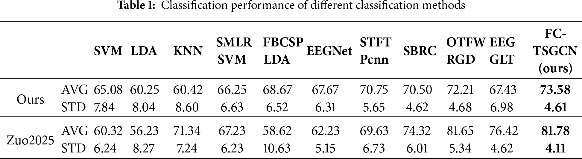
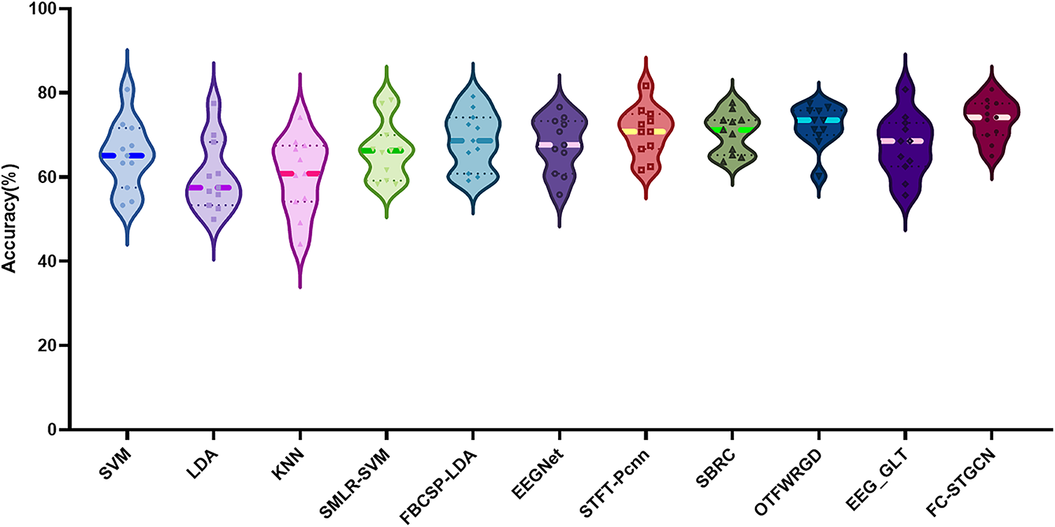
Figure 3: Accuracy of different methods on internal datasets

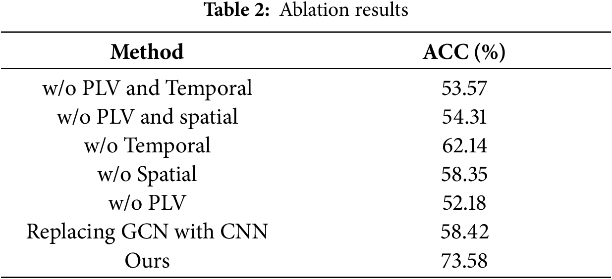
We conducted ablation studies on each module of our method. Table 2 presents the results. When temporal and spatial convolutions were not used, we replaced them with a conventional CNN.

5.2 Functional Connectivity

This study takes 9 electrodes as nodes and constructs a 9 on each of the 5 frequency bands × The symmetric adjacency matrix of 9 is used to observe the difference between the left and right foot MI, with each element representing the PLV between a pair of channels. Fig. 4 shows the adjacency matrix of subject P1 on five frequency bands during left foot (LF) and right foot (RF) MI execution.

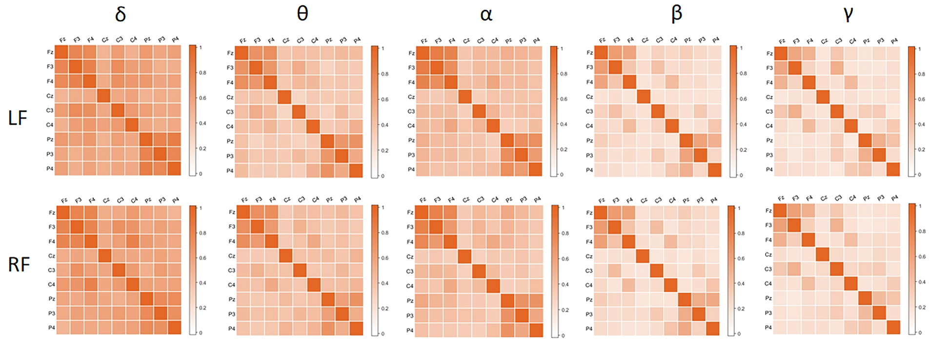
Figure 4: Functional connectivity matrix for different frequency bands

From the figure, it can be seen that the frequency band produces the highest intensity of coupling, while the frequency band β produces the lowest intensity of coupling. The five frequency bands exhibit similar coupling distributions. Both left and right foot MI tasks exhibit a highly coupled state in the frontal lobe region (Fz, F3, F4), as the frontal lobe is the advanced center of movement. The parietal cortex (Pz, P3, P4) also exhibits a high coupling state, indicating that the visual cortex may also be involved in some tasks.

Due to the presence of noise in EEG signals, there may be false connections between channels. In order to display the connectivity between channels more intuitively, this article will perform threshold processing on the adjacency matrix to screen out channel pairs with connectivity below 0.2. Then, paired t-tests were performed on the task state and resting state to detect channel pairs with significant differences. Finally, 3D brain maps of the left and right feet before and after processing were drawn. From top to bottom, there are left and right feet, including side view, back view, and inter view.

Comparing the left and right feet in Fig. 5, these connections are generally located in the motor cortex and visual cortex, but they are almost indistinguishable. By comparing the left and right feet in Fig. 6, it can be observed that the left foot MI exhibits stronger connectivity in the parietal lobe region, reflected in the P3-Pz channel pairing; The right foot MI exhibits stronger connectivity in the frontal lobe region, particularly in channel pairs F3-C3, F3-C4, F4-C3, F4-C4, and C3-C4. The connectivity of left foot MI in the front and rear of the brain is almost equal, while the connectivity of right foot MI between the channels in the front of the brain is much higher than that in the rear. In addition, both the left and right feet have connections that span the left and right hemispheres. These results indicate that there is mutual cooperation between brain regions during lower limb MI, which coincides with the viewpoint proposed by Phang and Ko [7] on the interdependence between the frontal, temporal, and parietal lobes during lower limb MI.

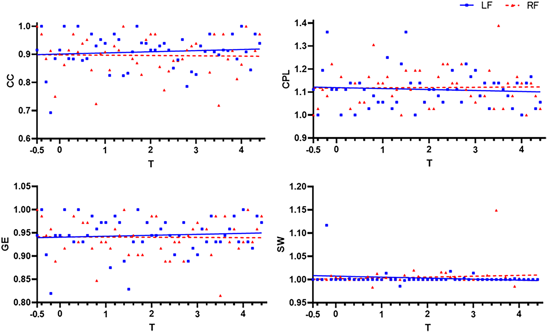
Figure 5: Comparison of CC, CPL, GE, and SW of left and right foot

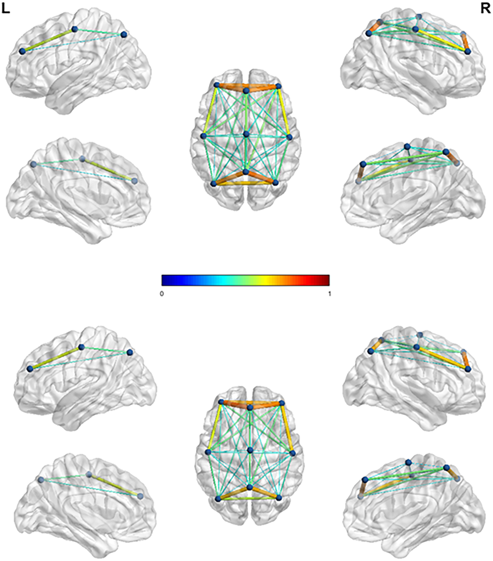
Figure 6: 3D brain functional connectivity mapping during left and right foot MI

5.3 Graph Theory Indicators

Figs. 4, 6 and 7 show the changes over time of the six graph-theoretic indicators introduced earlier. The blue square and red triangle in Fig. 4 represent the left and right feet, respectively. The solid blue line and the dashed red line represent the trend line of linear fitting, respectively.

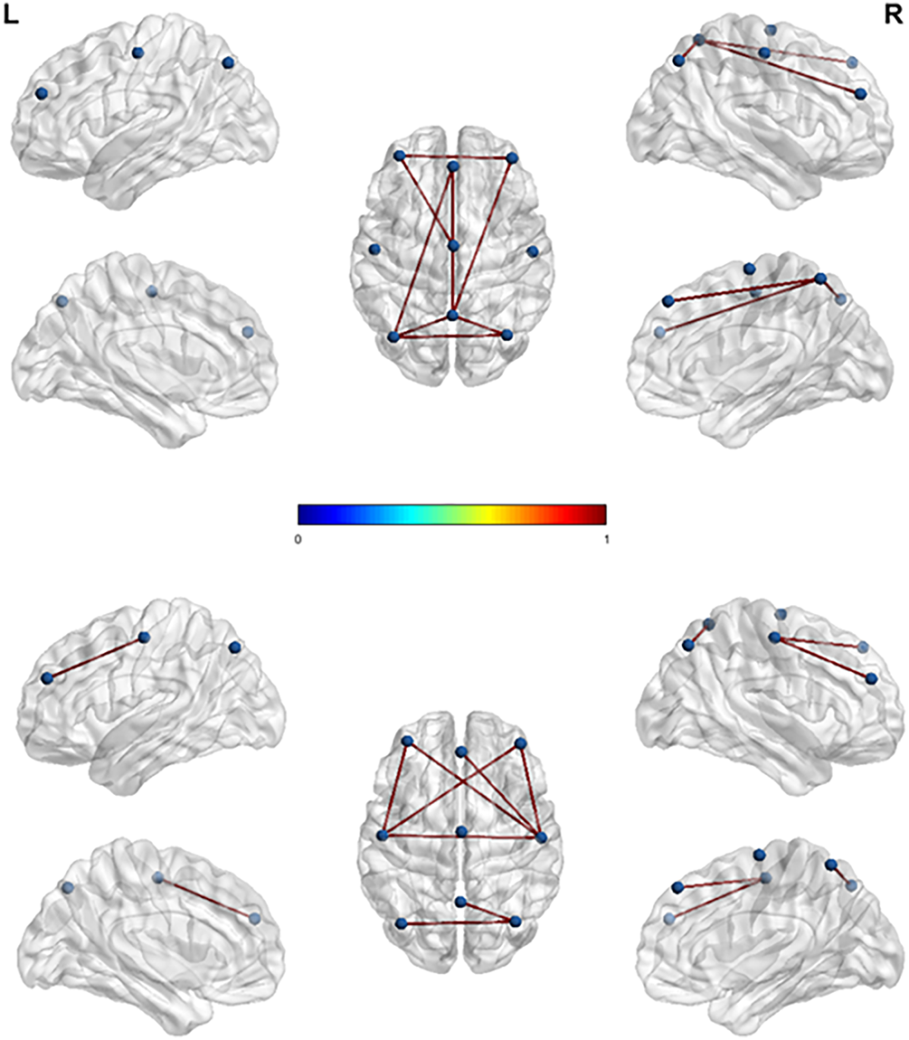
Figure 7: A paired t-test was performed between the task state and the resting state. Channel pairs with significant differences were selected

CC describes functional differentiation. From the upper left part of Fig. 4, it can be seen that CC of the left foot shows an upward trend over time, while CC of the right foot shows a slight downward trend over time. CC of the left foot is slightly higher than that of the right foot, indicating that when performing left foot MI, the connections between different brain regions are closer and the transmission ability of local information is stronger. However, there is no significant difference in the CC between the two tasks (Paired t-test, p = 0.329).

CPL and GE describe functional integration. From the upper right and lower left parts of Fig. 4, it can be seen that CPL of the left foot shows a decreasing trend over time, while the GE shows an upward trend; CPL of the right foot shows a slight upward trend over time, while the GE shows a slight downward trend. The decrease in CPL and the increase in GE mean an increase in information transmission and interaction efficiency between different brain regions. Paired t-tests showed no significant difference in CPL and GE between the two tasks (Paired t-test, p = 0.620 and p = 0.616). The calculation of SW attributes is closely related to CC and CPL, which can simultaneously reflect the ability of brain functional differentiation and integration. From the bottom right part of Fig. 4, it can be observed that both the left and right feet display SW attributes, especially during the 1–3 s period. This means that the brain can efficiently process left and right foot MI tasks. Similarly, there was no significant difference between the two tasks (Paired t-test, p = 0.605).

DC and BC describe the importance of different nodes. Fig. 8 shows the DC of the 9 channels on the left and right feet over time, with darker colors indicating lower importance. From the left figure, it can be seen that in the resting state of the left foot, except for Fz, Cz, and P4, the DC of all other channels is relatively consistent. Over time, C3 and C4 gradually become important, meaning that information begins to be transmitted through the central region. Finally, the MI task ended and each channel exhibited an approximate DC distribution. From the figure on the right, it can be seen that the DC of each channel in the right foot is relatively consistent in the resting state and at the end of the MI, while during the MI task, the DC of Fz, F4, Cz, C3, C4, Pz, and P3 remained ahead for a period of time.

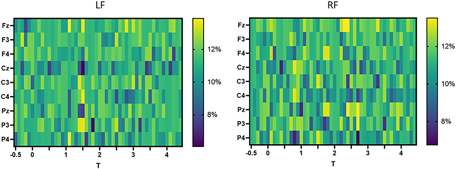
Figure 8: Comparison of DC of left and right foot

Fig. 9 shows the variation of the BC of the 9 channels on the left and right feet over time, with darker colors indicating lower importance. From the left figure, it can be seen that the BC of each channel is relatively low at the beginning. During the MI task, the BC of Fz, C3, Pz, and P4 was high, indicating that these nodes assumed the role of “bridges”. As the MI task approaches its end, each channel exhibits an approximate end centrality distribution. From the figure on the right, it can be seen that except in the later stage of the MI task, the BC of Pz and P3 has taken the lead, and the BC of each channel in the right foot is relatively consistent at other times, without any particularly important nodes.

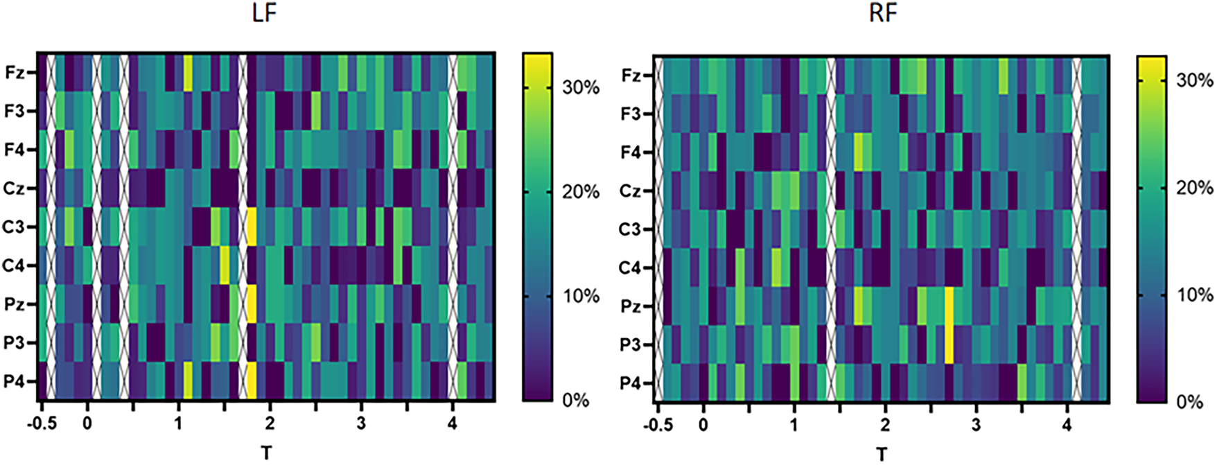
Figure 9: Comparison of BC of left and right foot

5.4 Limitations and Future Work

The sample size in this study was relatively small. With a larger sample size and broader demographic representation (e.g., differences in gender, age, health status), the classification results may yield more robust outcomes. Plans include recruiting more participants across different genders, ages, ethnicities, and health statuses to enhance the model’s robustness to individual variations. While the convolution-based architecture with spatiotemporal convolutions offers accuracy advantages, it may incur higher computational time and resource consumption. This could pose challenges for real-time BCI systems with stringent latency and computational resource constraints. Future efforts should focus on optimizing model parameter size and reducing latency through techniques like pruning, distillation, sparsification, and quantization, enabling deployment in real-time BCI systems or embedded environments. Additionally, to enhance modeling of spatial or spectral dependencies, integrating attention layers into graph convolutions or adopting hybrid Transformer-GCN models could improve the capture of critical channel or connection importance.

6  Conclusion

This study proposes a classification method for lower limb MI-EEG signals, which uses phase-locked values to construct functional connection matrices as features of the left and right legs and then uses temporal-spatial graph convolutional networks to capture temporal and spatial information for classification. This study designed a lower limb EEG acquisition experiment and established an in-house dataset for subsequent performance evaluation and functional brain network analysis. The classification results show that the proposed method achieved an average accuracy of 73.58% and the highest accuracy of 80.83%, which is higher than the existing methods. At the same time, the standard deviation is also the lowest among all methods, demonstrating the potential for application in BCI control systems. In addition, this study analyzed the brain network based on graph-theoretic indicators, revealing the brain network mechanism during left and right foot MI, which may help find new strategies to improve MI-BCI performance.

Acknowledgement: The authors would like to thank all the volunteers who participated in the experiments.

Funding Statement: This work was supported in part by the National Natural Science Foundation of China under Grant 62172368, and the Natural Science Foundation of Zhejiang Province under Grant LR22F020003.

Author Contributions: Study conception and design: Yang Liu, Qi Lu, Shiwei Cheng; data collection: Qi Lu; analysis and interpretation of results: Qi Lu; draft manuscript preparation: Yang Liu, Junjie Wu, Huaichang Yin. All authors reviewed the results and approved the final version of the manuscript.

Availability of Data and Materials: The data will be available on reasonable request.

Ethics Approval: The participants signed an informed consent form. EEG was recorded from 10 participants, where the authors work collaborated with Zhejiang Hospital, China. The Ethics Committee of the Zhejiang Hospital approved the study (Approval No. 2025-C-095).

Conflicts of Interest: The authors declare no conflicts of interest to report regarding the present study.

References

1. Liu Z, Wang L, Xu S, Lu K. A multiwavelet-based sparse time-varying autoregressive modeling for motor imagery EEG classification. Comput Biol Med. 2023;155(2):106196. doi:10.1016/j.compbiomed.2022.106196. [Google Scholar] [PubMed] [CrossRef]

2. Abenna S, Nahid M, Bouyghf H, Ouacha B. An enhanced motor imagery EEG signals prediction system in real-time based on delta rhythm. Biomed Signal Process Control. 2023;79:104210. doi:10.1016/j.bspc.2022.104210. [Google Scholar] [CrossRef]

3. Roy AM. An efficient multi-scale CNN model with intrinsic feature integration for motor imagery EEG subject classification in brain-machine interfaces. Biomed Signal Process Control. 2022;74(4):103496. doi:10.1016/j.bspc.2022.103496. [Google Scholar] [CrossRef]

4. Penfield W, Boldrey E. Somatic motor and sensory representation in the cerebral cortex of man as studied by electrical stimulation. Brain. 1937;60(4):389–443. doi:10.1093/brain/60.4.389. [Google Scholar] [CrossRef]

5. Jeffery DT, Norton JA, Roy FD, Gorassini MA. Effects of transcranial direct current stimulation on the excitability of the leg motor cortex. Exp Brain Res. 2007;182(2):281–7. doi:10.1007/s00221-007-1093-y. [Google Scholar] [PubMed] [CrossRef]

6. Murphy DP, Bai O, Gorgey AS, Fox J, Lovegreen WT, Burkhardt BW, et al. Electroencephalogram-based brain-computer interface and lower-limb prosthesis control: a case study. Front Neurol. 2017;8:696. doi:10.3389/fneur.2017.00696. [Google Scholar] [PubMed] [CrossRef]

7. Phang CR, Ko LW. Global cortical network distinguishes motor imagination of the left and right foot. IEEE Access. 2020;8:103734–45. doi:10.1109/access.2020.2999133. [Google Scholar] [CrossRef]

8. Yan S, Xiong Y, Lin D. Spatial temporal graph convolutional networks for skeleton-based action recognition. Proc AAAI Conf Artif Intell. 2018 Apr;32(1):7444–52. doi:10.1609/aaai.v32i1.12328. [Google Scholar] [CrossRef]

9. Gu L, Yu Z, Ma T, Wang H, Li Z, Fan H. EEG-based classification of lower limb motor imagery with brain network analysis. Neuroscience. 2020;436(12):93–109. doi:10.1016/j.neuroscience.2020.04.006. [Google Scholar] [PubMed] [CrossRef]

10. Tariq M, Trivailo PM, Simic M. Classification of left and right foot kinaesthetic motor imagery using common spatial pattern. Biomed Phys Eng Express. 2019;6(1):015008. doi:10.1088/2057-1976/ab54ad. [Google Scholar] [PubMed] [CrossRef]

11. Lu B, Ge S, Wang H. EEG-based classification of lower limb motor imagery with STFT and CNN. In: Neural Information Processing. Cham, Switzerland: Springer; 2021. p. 397–404. doi:10.1007/978-3-030-92310-5_46. [Google Scholar] [CrossRef]

12. Sun X, Liu T, Wang K, Pan L, Meng L, Ding X, et al. Enhance decoding of lower limb motor imagery-electroencephalography patterns by Riemannian clustering. Interdiscipl Med. 2025;3(4):e20250003. doi:10.1002/inmd.20250003. [Google Scholar] [CrossRef]

13. Li P, Liu H, Si Y, Li C, Li F, Zhu X, et al. EEG based emotion recognition by combining functional connectivity network and local activations. IEEE Trans Biomed Eng. 2019;66(10):2869–81. doi:10.1109/tbme.2019.2897651. [Google Scholar] [PubMed] [CrossRef]

14. Chen X, Zhang H, Gao Y, Wee CY, Li G, Shen D, et al. High-order resting-state functional connectivity network for MCI classification. Hum Brain Mapping. 2016;37(9):3282–96. doi:10.1002/hbm.23240. [Google Scholar] [PubMed] [CrossRef]

15. Liu L, Zeng LL, Li Y, Ma Q, Li B, Shen H, et al. Altered cerebellar functional connectivity with intrinsic connectivity networks in adults with major depressive disorder. PLoS One. 2012;7(6):e39516. doi:10.1371/journal.pone.0039516. [Google Scholar] [PubMed] [CrossRef]

16. Cohen I, Huang Y, Chen J, Benesty J, Benesty J, Chen J, et al. Pearson correlation coefficient. Noise Reduction Speech Process. 2009:1–4. doi:10.1007/978-3-642-00296-0_5. [Google Scholar] [CrossRef]

17. Fan E. Extended tanh-function method and its applications to nonlinear equations. Phys Lett A. 2000;277(4–5):212–8. doi:10.1016/s0375-9601(00)00725-8. [Google Scholar] [CrossRef]

18. Meng XL, Rosenthal R, Rubin DB. Comparing correlated correlation coefficients. Psychol Bull. 1992;111(1):172. doi:10.1037/0033-2909.111.1.172. [Google Scholar] [CrossRef]

19. Jöreskog KG. A general method for analysis of covariance structures. Biometrika. 1970;57(2):239–51. doi:10.1093/biomet/57.2.239. [Google Scholar] [CrossRef]

20. Stam CJ, Nolte G, Daffertshofer A. Phase lag index: assessment of functional connectivity from multi channel EEG and MEG with diminished bias from common sources. Hum Brain Mapping. 2007;28(11):1178–93. doi:10.1002/hbm.20346. [Google Scholar] [PubMed] [CrossRef]

21. Jian W, Chen M, McFarland DJ. EEG based zero-phase phase-locking value (PLV) and effects of spatial filtering during actual movement. Brain Res Bulletin. 2017;130(11):156–64. doi:10.1016/j.brainresbull.2017.01.023. [Google Scholar] [PubMed] [CrossRef]

22. Nolte G, Bai O, Wheaton L, Mari Z, Vorbach S, Hallett M. Identifying true brain interaction from EEG data using the imaginary part of coherency. Clin Neurophysiol. 2004;115(10):2292–307. doi:10.1016/j.clinph.2004.04.029. [Google Scholar] [PubMed] [CrossRef]

23. Carter G, Knapp C, Nuttall A. Estimation of the magnitude-squared coherence function via overlapped fast Fourier transform processing. IEEE Trans Audio Electroacoust. 1973;21(4):337–44. doi:10.1109/tau.1973.1162496. [Google Scholar] [CrossRef]

24. Wang H, Xu T, Tang C, Yue H, Chen C, Xu L, et al. Diverse feature blend based on filter-bank common spatial pattern and brain functional connectivity for multiple motor imagery detection. IEEE Access. 2020;8:155590–601. doi:10.1109/access.2020.3018962. [Google Scholar] [CrossRef]

25. Jin SH, Lin P, Auh S, Hallett M. Abnormal functional connectivity in focal hand dystonia: mutual information analysis in EEG. Movement Disorders. 2011;26(7):1274–81. doi:10.1002/mds.23675. [Google Scholar] [PubMed] [CrossRef]

26. King JT, John AR, Wang YK, Shih CK, Zhang D, Huang KC, et al. Brain connectivity changes during bimanual and rotated motor imagery. IEEE J Transl Eng Health Med. 2022;10:1–8. doi:10.1109/jtehm.2022.3167552. [Google Scholar] [PubMed] [CrossRef]

27. Gu L, Yu Z, Ma T, Wang H, Li Z, Fan H. Random matrix theory for analysing the brain functional network in lower limb motor imagery. In: 2020 42nd Annual International Conference of the IEEE Engineering in Medicine & Biology Society (EMBC); 2020 Jul 20–24; Montreal, QC, Canada. p. 506–9. [Google Scholar]

28. Shi K, Huang R, Lyu J, Li Z, Mu F, Peng Z, et al. EEG-based motor imagery classification with tuned heuristic fusion graph convolutional network for rehabilitation training. IEEE Trans Autom Sci Eng. 2025;22(2):14928–39. doi:10.1109/tase.2025.3564162. [Google Scholar] [CrossRef]

29. Demir A, Koike-Akino T, Wang Y, Haruna M, Erdogmus D. EEG-GNN: graph neural networks for classification of electroencephalogram (EEG) signals. In: 2021 43rd Annual International Conference of the IEEE Engineering in Medicine & Biology Society (EMBC); 2021 Nov 1–5; Mexico. p. 1061–7. [Google Scholar]

30. Xiao Z, Liang W, Dai W. Research on lower limb movement rehabilitation assessment based on graph convolutional network. IEEE Access. 2024;12(11):169194–207. doi:10.1109/access.2024.3491862. [Google Scholar] [CrossRef]

31. Sun B, Zhang H, Wu Z, Zhang Y, Li T. Adaptive spatiotemporal graph convolutional networks for motor imagery classification. IEEE Signal Processing Letters. 2021;28:219–23. doi:10.1109/lsp.2021.3049683. [Google Scholar] [CrossRef]

32. Defferrard M, Bresson X, Vandergheynst P. Convolutional neural networks on graphs with fast localized spectral filtering. In: NIPS’16: Proceedings of the 30th International Conference on Neural Information Processing Systems; 2016 Dec 5–10; Barcelona Spain. p. 3844–52. [Google Scholar]

33. Li Q, Han Z, Wu XM. Deeper insights into graph convolutional networks for semi-supervised learning. Proc AAAI Conf Artif Intell. 2018;32(1):3538–45. doi:10.1609/aaai.v32i1.11604. [Google Scholar] [CrossRef]

34. Song T, Zheng W, Song P, Cui Z. EEG emotion recognition using dynamical graph convolutional neural networks. IEEE Trans Affect Comput. 2018;11(3):532–41. doi:10.1109/taffc.2018.2817622. [Google Scholar] [CrossRef]

35. Yang S, Li M, Wang J. Fusing sEMG and EEG to increase the robustness of hand motion recognition using functional connectivity and GCN. IEEE Sensors J. 2022;22(24):24309–19. doi:10.1109/jsen.2022.3221417. [Google Scholar] [CrossRef]

36. You Y, Chen T, Wang Z, Shen Y. L2-gcn: layer-wise and learned efficient training of graph convolutional networks. In: Proceedings of the IEEE/CVF Conference on Computer Vision and Pattern Recognition; 2020 Jun 13–19; Seattle, WA, USA. p. 2127–35. [Google Scholar]

37. Liu YH, Lin LF, Chou CW, Chang Y, Hsiao YT, Hsu WC. Analysis of electroencephalography event-related desynchronisation and synchronisation induced by lower-limb stepping motor imagery. J Med Biol Eng. 2019;39(1):54–69. doi:10.1007/s40846-018-0379-9. [Google Scholar] [CrossRef]

38. Hearst MA, Dumais ST, Osuna E, Platt J, Scholkopf B. Support vector machines. IEEE Intell Systr Appl. 1998;13(4):18–28. doi:10.1109/5254.708428. [Google Scholar] [CrossRef]

39. Fisher RA. The use of multiple measurements in taxonomic problems. Ann Eugen. 1936;7(2):179–88. doi:10.1111/j.1469-1809.1936.tb02137.x. [Google Scholar] [CrossRef]

40. Cover T, Hart P. Nearest neighbor pattern classification. IEEE Trans Inf Theory. 1967;13(1):21–7. doi:10.1109/tit.1967.1053964. [Google Scholar] [CrossRef]

41. Lawhern VJ, Solon AJ, Waytowich NR, Gordon SM, Hung CP, Lance BJ. EEGNet: a compact convolutional neural network for EEG-based brain-computer interfaces. J Neural Eng. 2018;15(5):056013. doi:10.1088/1741-2552/aace8c. [Google Scholar] [PubMed] [CrossRef]

42. Zuo C, Yin Y, Wang H, Zheng Z, Ma X, Yang Y, et al. Enhancing classification of a large lower-limb motor imagery EEG dataset for BCI in knee pain patients. Sci Data. 2025;12(1):1451. doi:10.1038/s41597-025-05767-2. [Google Scholar] [PubMed] [CrossRef]

43. Aung HW, Li JJ, Shi B, An Y, Su SW. EEG_GLT-Net: optimising EEG graphs for real-time motor imagery signals classification. Biomed Signal Process Control. 2025;104(6):107458. doi:10.1016/j.bspc.2024.107458. [Google Scholar] [CrossRef]

44. Watts DJ, Strogatz SH. Collective dynamics of ‘small-world’ networks. Nature. 1998;393(6684):440–2. doi:10.1038/30918. [Google Scholar] [PubMed] [CrossRef]