Graph Guide Diffusion Solvers with Noises for Travelling Salesman Problem

1  Introduction

Combinatorial Optimization (CO) represents a category of mathematical optimization problems distinguished by a solution space comprising a finite number of discrete candidate solutions, typically formed from combinations of a limited set of objects, such as numbers, items, nodes, etc. The objective of CO is to identify an optimal solution among these discrete candidates such that the specified objective function attains either its maximum or minimum value while adhering to certain constraints. As an Non-deterministic Polynomial-time hard (NP-hard) problem, CO primarily depends on expert knowledge and handcrafted heuristic methods to approximate the optimal solution [1]. The Traveling Salesman Problem (TSP), a classic challenge in the field of CO, is defined as follows: Given a group of cities and the distance between each pair of cities, the TSP requires finding the shortest path so that the traveling salesman visits each city exactly once and eventually returns to the starting one. The TSP has extensive real-world applications, such as optimizing routes in logistics and supply chain management [2], as well as in the domain of traffic management [3], among other uses. The TSP has many variants that introduce additional constraints and complexities, making it more applicable to real-world scenarios. One such variant is the Generalized Traveling Salesman Problem (GTSP), where cities are grouped into clusters, and the salesman must visit exactly one city from each cluster [4]. Another variant is the Multiple Traveling Salesmen Problem (mTSP), where multiple salesmen start from a common depot, visit different cities, and return to the depot [5].

In recent years, the rapid advancement of Deep Learning (DL) has significantly contributed to progress in CO. Conventional methods for tackling CO issues are typically categorized into three groups, differentiated by their solution generation strategies: (1) Methods that construct solutions in an Autoregressive (AR) manner, (2) Those that employ Non-Autoregressive (NAR) approaches, and (3) Heuristic-based solvers that focus on improving existing solutions. The core idea of AR solvers is to treat the problem solution as a sequential process, where partial solutions are constructed step by step, with each decision conditioned on the previous outputs (see, e.g., the pointer-based autoregressive framework proposed in [6] and the attention-based autoregressive model in [7] for TSP and related routing problems). Since each decision must consider the results of all prior steps, this makes it difficult to scale to larger problems. Next, we have NAR solvers, which differ from AR solvers primarily in the way solutions are generated. NAR solvers typically rely on the assumption of conditional independence, where each part of the solution can be decided independently. This assumption enables the solver to parallelize the calculation of each part of the solution, producing the entire solution in a single step. However, because of this simplified assumption, NAR solvers ignore the potential dependencies between different parts of the solution, which may lead to suboptimal final results [8–11]. The third method starts with an initial feasible solution and applies local search strategies (such as the simulated annealing method [12] among others) to fine-tune it, iterating until a feasible solution is found [13]. This approach combines the efficiency of heuristic algorithms with the learning capabilities of Neural Networks (NNs) to find better solutions, often used as a post-processing step to optimize an initial solution and improve the final outcome. By comparing these three methods, we can see that each has its own advantages and limitations. Combining the strengths of DL with traditional optimization methods holds great promise for providing more powerful solutions to CO problems.

Many traditional Neural Combinatorial Optimization (NCO) solvers based on NNs aim to minimize the average objective function across all training instances during the training process [6,7]. However, in pursuit of overall average performance, this approach may sacrifice optimal solutions for some instances, particularly those that are edge cases differing significantly from the majority of the data. To solve this problem, Sun and Yang [14] introduced Diffusion Solvers for Combinatorial Optimization (DIFUSCO), a graph-based diffusion solver that utilizes the capability of diffusion models to learn and produce high-quality solution distributions for various problem instances. Diffusion models, one of the rapidly developing generative models in recent years [15,16], are particularly well-suited to solve the above problem. These models are capable of learning the fundamental distribution of data, enabling them to generate new data samples. In the realm of CO problems, DIFUSCO has shown strong performance in solving TSP and Maximal Independent Set (MIS) problems. However, a key issue with current approaches is the use of fixed noise schedules for noise generation, such as linear or cosine annealing schedules [17]. These noise schedules are independent of the specific graph structure. In the case of TSP, for example, each problem instance is unique, especially for the edge cases with distinct characteristics. Therefore, it is crucial to control the noise level based on the graph structure of each instance to better handle the diversity and complexity of graph structures. By carefully designing the noise schedule, the efficiency and quality of the model’s generation can be improved [18,19]. A well-designed dynamic noise schedule [20] is essential for more effectively exploring the solution space during the denoising process, reducing unnecessary search, and ultimately enhancing overall search efficiency.

Based on this, we propose a learnable noise scheduling method. Specifically, by integrating Graph Neural Networks (GNNs) with an information propagation mechanism, the noise levels in the diffusion model are dynamically adjusted, particularly tailored for the TSP. The proposed method, termed Graph-Guided Diffusion Solvers (GGDS) for CO, utilizes GNNs to capture structural information encoded in city coordinates and the adjacency matrix, and subsequently generates a noise schedule conditioned on the graph structure. The core of GGDS lies in the noise schedule generated by the Graph Neural Network (GNN), which encapsulates information about the graph structure. This means that the noise injection process takes into account the inherent structure of the problem. Such noise injection helps preserve the graph structure during the denoising process, enabling a more accurate reconstruction of solutions that align with the structural characteristics of the graph. When the noise schedule is closely tied to the graph structure, each step in the denoising process is more likely to move toward the optimal solution. This method, which combines the graph structure-awareness of GNN with the flexible noise adjustment mechanism of diffusion models, offers a novel perspective for solving CO problems. By incorporating gradient feedback from the target optimization in the denoising steps, GGDS can efficiently reconstruct low-cost solutions while enhancing the diffusion process.

To summarize, we identify a key limitation of existing diffusion-based CO solvers: their instance-agnostic, fixed noise schedules inevitably diminish graph-specific features. GGDS addresses this bottleneck by incorporating a lightweight GNN that adjusts the noise levels according to the graph structure of the problem instance. As a result, GGDS transforms the noise schedule into a learnable, structure-aware component, providing a novel approach to solving combinatorial optimization problems. GGDS learns an instance-specific noise schedule via a lightweight GNN, fuses it with the temporal schedule, and boosts TSP solution quality by up to 88.7% without extra inference cost.

2  Related Work

In this part of the document, we offer a summary of conventional approaches to addressing CO problems, as well as insights into recent developments in NCO methods and the evolution of diffusion-based models. As for the CO problem-solving techniques, they are generally divided into two main types depending on their solution generation process: those that build solutions from scratch, known as construction solvers, and those that refine existing solutions, referred to as improvement solvers.

2.1 Construction Solver

Constructed solvers can be classified into AR and NAR types depending on how they generate the solution. AR models build the solution step by step during decoding, progressively adding one node at a time to the partial solution until a full solution to the TSP problem is obtained. In [21], the authors were the first to combine Pointer Networks (PtrNet) [6] with Deep Reinforcement Learning (DRL), achieving state-of-the-art (SOTA) results. Furthermore, Kool et al. [7] used Attention Models (AM) to address related routing problems, and Kwon et al. [22] further expanded on these AM by leveraging symmetry in Reinforcement Learning (RL) methods, introducing the Policy Optimization with Multiple Optima (POMO) model to address the issue of multiple optimal solutions in AM models. Pan et al. [23] proposed a hierarchical framework, H-TSP, based on DRL. It utilizes a strategy of breaking down extensive issues into smaller, more easily handled sub-tasks through a divide-and-conquer approach, solving each subproblem separately. This method effectively resolves the problem of inefficiency when solving large-scale TSP instances. However, since AR models require step-by-step computation of outputs at each step, where each step’s output depends on the previous step’s result, the inference speed tends to slow down. In contrast, NAR models typically generate the entire solution in one step. For instance, Joshi et al. [9] used deep Graph Convolutional Networks (GCN) to construct efficient TSP graph representations and employed highly parallelized beam search to output the solution path for the Euclidean TSP problem in a NAR manner. Asani et al. [24] propose an innovative constructive heuristic algorithm, the Half Max Insertion Heuristic (HMIH), for solving the TSP. This method effectively reduces the cost of path growth by constructing an initial sub-tour and iteratively inserting nodes that satisfy the “half maximum distance” criterion. Xiao et al. [25] first proposed a RL-based NAR model for solving the TSP. By leveraging a specialized GNN architecture and an enhanced RL strategy, the model efficiently solves the TSP while maintaining solution quality and strong generalization ability. Although this NAR model accelerates the decoding process by assuming conditional independence, it neglects the potential dependencies between different parts of the solution, which may lead to suboptimal performance. Recently, Fu et al. [26] improved the solution capability of the NAR model by constructing heatmaps and incorporating Monte Carlo Tree Search (MCTS). While MCTS can effectively explore the solution space, its high time complexity may result in longer runtime. Additionally, the accuracy and sparsity issues of the heatmaps can affect the search efficiency and solution quality of MCTS. The limitations of MCTS’s sampling strategy and search depth could also lead to local optima, thus reducing the quality of the solutions.

2.2 Improvement Solver

In contrast to constructed solvers, there are improved solvers, which iteratively optimize the results obtained by previous algorithms to search for better solutions. For example, Costa et al. [27] proposed a policy gradient algorithm that learns a heuristic strategy based on the 2-Optimization (2OPT) operation. This strategy selects when to apply the 2OPT operation given the current solution, and by combining DRL with the 2OPT operation, it effectively improves the solution quality for the TSP. But the 2OPT operation incurs significant computational overhead in large-scale TSP instances and primarily focuses on optimizing path length, making it unsuitable for directly handling TSP variants with additional constraints. Traditional Genetic Algorithms (GA) can enhance the quality of TSP solutions by employing suitable crossover operators. For instance, Rani and Kumar [28] proposed a genetic algorithm that incorporates improved crossover and mutation strategies to optimize TSP path solutions. Their method, which utilizes the Order Crossover 6 (OX6) operator and inversion mutation, outperforms traditional GA approaches in terms of both convergence speed and accuracy, as demonstrated on the TSPLIB dataset. This approach provides a valuable reference for improvement-based heuristic algorithms. Additionally, the Composite Sequence Crossover (CSCX1) introduced by Ahmed et al. [29] is another example of such methods. These algorithms fall within the category of improvement-based solvers, typically beginning with an initial population and progressively refining solutions through crossover and mutation operations.

2.3 Diffusion Probabilistic Models

The use of generative models for solving CO problems has garnered growing interest in recent years. A notable example is [30], which introduced a generative model for the Vehicle Routing Problem (VRP). The diffusion model [31], as a generative model, has also attracted considerable attention from researchers. By gradually introducing Gaussian noise to clean data in the forward process and learning to remove the noise in the reverse process, the model learns to capture the distribution of high-quality solutions. This allows the diffusion model to produce new sample data which are similar to the training data. Recent studies have shown that diffusion models have demonstrated immense potential in video generation [32,33], audio generation [34], and text generation [35,36]. Furthermore, Du et al. [37] applied diffusion models to decompose the Global Routing (GR) problem into two phases: the hub-generation phase and the pin-hub-connection phase. This approach effectively addresses a core and time-consuming challenge in Very Large-Scale Integration (VLSI) design. More recently, research by [14] demonstrated that applying diffusion models to CO problems can still yield highly effective results, contributing to new advancements in the field.

In this work, the GGDS can be viewed as a type of NAR-based constructive solver, which iteratively optimizes the final solution using a diffusion model. Unlike existing methods [14], GGDS not only incorporates time step information in the noise schedule but also introduces graph structural information.

3  Proposed Method

3.1 Preliminaries: Diffusion Models for TSP

3.1.1 Problem Definition

Consistent with the definitions of CO problems in [14,38], we represent an instance of the CO problem by a graph G=(V,E), where V and E respectively represent the set of vertices and edges, in the graph. Following standard notation in [39], we define χs={0,1}N as the solution space for an instance s of the CO problem, where N is the number of edges in the graph G, and cs(x)=cost(x,s) as the cost of an instance s given a solution x, where x∈χs. The present study concentrates on a quintessential CO issue: the TSP. An instance of TSP is established on an undirected, complete graph G=(V,E), with V denoting the collection of nodes that include n cities. In the edge set E, each element eij carries a non-negative weight, signifying the Euclidean distance between cities i and j. A TSP route is represented as an ordering of the n city nodes, expressed as π={π1,π2,…,πn}, where πi≠πj, ∀i≠j. Consequently, the TSP is framed as the quest for a route within G that constitutes a Hamiltonian cycle, aiming to minimize the aggregate weight of the cities along the cycle.

Within this study, we conceptualize the TSP as an issue involving the selection of edges. The solution space, denoted by χs, is composed of binary indicators xij that signify the inclusion of edge (i,j) within the solution set x. The associated cost is determined through the formula: cs(x)=Σixi⋅wi(s), with wi(s) denoting the weight attributed to edge i within instance s. The aim of the CO problem is to identify an best and feasible solution xs∗ for a specific instance s, characterized by: xs∗=argminx∈χs cs(x), which essentially involves reducing the cost associated with instance s to its minimum.

3.1.2 Diffusion Model in CO Problem

Based on the design in [14], this work applies the diffusion model to generate solutions for the CO problem, treating it as a generative task, pθ(x|G) represents the finally generated probability distribution of the solution x given a specific problem instance graph G. The diffusion model comprises a forward noise-adding process and a reverse denoising process. The forward noise-adding process, known as the diffusion process, starts with the original data q(x0) and gradually adds noise, creating a sequence of latent variables x1:T=x1,x2,…,xT. The formal expression for this process can be written as:

q(x1:T|x0)=Πt=1Tq(xt|xt−1)(1)

where the term q(xt|xt−1) represents the process of progressively corrupting the data at time step t−1 to obtain the latent variable at the next time step t. On the other hand, the denoising process begins with the final latent variable p(xT) and gradually eliminates the noise to reconstruct the clean data, eventually reaching the target data distribution. This denoising process can be formally described as:

pθ(x0:T)=p(xT)Πt=1Tpθ(xt−1|xt)(2)

where pθ(xt−1|xt) represents the conditional probability for the reverse process, which gradually transforms the latent variable back to the original data distribution. This denoising process is learned by the model, where θ denotes the model parameters.

A primary goal in training the model is to ensure that the distribution pθ(x0|G), as learned by the model, closely mirrors the actual data distribution q(x0|G). This objective is commonly realized by optimizing the negative log-likelihood, expressed as follows:

Lreconstruction=E[−log⁡pθ(x0)]≤Eq(x1:T|x0)[∑t>1DKL(q(xt−1|xt,x0)||pθ(xt−1|xt))−log⁡pθ(x0|x1)]+C(3)

where, C signifies a constant, and DKL denotes the Kullback-Leibler (KL) divergence, a metric for assessing the divergence between the distribution predicted by the model and the actual distribution.

3.1.3 Forward Time Diffusion Process

In this work, we follow the approach outlined in [14], but focus exclusively on the discrete diffusion model. In the discrete diffusion model, the forward noise-adding process is defined as:

q(xt|xt−1)=Cat(xt;p=x~t−1Qt)(4)

where the transition probability matrix Qt is of the form:

Qt=[(1−βt)βtβt(1−βt)](5)

with Qtε[0,1]2×2. This matrix defines the probability of transitioning from one time step to another in the diffusion model, where βt controls the degree of noise introduced at each step, representing the corruption rate of the data. The parameter βt lies between 0 and 1, and 1−βt represents the proportion of original information retained at each time step.

In the context of the CO problem, the solution vector can be expressed as χs={0,1}N, and here, x~ is the extended vector of χs, i.e., x~t∈{0,1}N×2, where each row is a one-hot vector. In specific, the noising process is achieved by multiplying x~ at step t with the transition matrix Qt. This operation gradually corrupts each row of x~t by flipping the active entry according to the probabilities defined in Qt, simulating the addition of noise. In the forward noising process of the discrete model, the goal is for the data to be progressively noised by polynomial noise until, at the final time step T, the original structure and information of the data are nearly entirely replaced by noise, with xT approaching a uniform distribution, i.e., xT∼Uniform(⋅). Thus, in the discrete diffusion model, after introducing noise over t steps starting from x0, the marginal distribution at step t is given by:

q(xt|x0)=Cat(xt;p=x~0Q¯t)(6)

where Q¯t=Q1Q2…Qt. The posterior distribution at step t−1 can be derived using Bayes’ theorem:

q(xt−1|xt,x0)=q(xt|xt−1,x0)q(xt−1|x0)q(xt|x0)=Cat(xt−1;p=x~tQtT⊙x~0Q¯t−1x~0Q¯tx~tT)(7)

The denoising Neural Network (NN) is trained to predict the clean data pθ(x~0|xt) from the noisy data xt. In the reverse diffusion process, at each iteration, the predicted x~0epoch for the current epoch is generated and used as x0 for the next step in Eq. (7). This procedure is repeated until all the predefined denoising steps have been completed. This process can be expressed as:

pθ(xt−1|xt)=∑x~0q(xt−1|xt,x~0)pθ(x~0|xt)(8)

3.1.4 Denoising and Decoding

In this study, the choice of denoising network and the design of the decoding strategy follow prior work [14,40]. In the decoding process, diffusion models generate the final predicted variables x through a gradual denoising process. Whether it is a continuous diffusion model that quantizes continuous variables to obtain predictions, or a discrete diffusion model that uses Bernoulli sampling to derive the final predicted variables, these direct prediction methods lose the confidence information for each variable. This confidence information is crucial for subsequent decoding tasks, such as conflict resolution. To retain this confidence information, we adjust the diffusion model as proposed in previous works [9,11,14] to generate heatmaps. Specifically, for the discrete diffusion model, we preserve the predicted probability of each variable being one (i.e., x0=1) as the heatmap score. In this way, each value in the heatmap reflects the model’s belief that the variable is 1. For the continuous diffusion model, we remove the final quantization step and instead use 0.5(x^0+1) as the heatmap score. This transformation maps the continuous variables to the [0, 1] range, representing the confidence for each variable. In this manner, the generated heatmap not only retains the confidence information for each predicted variable but also provides greater flexibility and diversity for the subsequent decoding process, aiding in more effective conflict resolution and optimization of the final solution. For the heatmap A, the element Aij represents the confidence of edge (i, j). We adopt a greedy decoding strategy.

3.2 Methodology: Noise Scheduling with GNN for TSP

3.2.1 The Necessity of Instance-Specific Noise Scheduling

In diffusion models, noise scheduling plays a crucial role in determining how noise is progressively added to the data. Previous studies [14] have typically employed fixed noise scheduling methods, such as linear increase or cosine annealing. However, these methods overlook significant differences in the complexity, sparsity, and local connectivity of various graph structures, which becomes particularly prominent in large-scale TSP instances. On one hand, during the early stages of diffusion, critical edges (such as those forming the shortest path) may lose their structural characteristics due to excessive perturbation, making it difficult to accurately recover these key structures during the reverse denoising phase. On the other hand, the uniform noise path fails to align with the specific structure of the graph, leading to redundant searches and reduced efficiency. Moreover, the fixed noise intensity results in inconsistent learning difficulties across different structural instances, which affects the stability of the training process.

As the problem scale increases, these shortcomings become more pronounced. In large-scale graph problems, the performance of fixed noise scheduling typically deteriorates sharply. As the number of nodes n increases, the size of the adjacency matrix grows at a rate of O(n2), which not only exacerbates the issue of excessive perturbation in sparse regions but also leads to insufficient exploration in dense areas. This phenomenon is particularly evident in large-scale TSP instances, where the graph’s topological complexity and the combinatorial optimization difficulty increase exponentially, making traditional noise scheduling mechanisms ill-suited to handle such high-dimensional and heterogeneous structural characteristics.

To address these challenges, the GGDS introduces a graph-guided noise scheduling mechanism. This mechanism leverages GNNs to extract key features from the graph structure and dynamically generate perturbation intensities tailored to each instance, thus enabling the customization of the forward diffusion path. Specifically, at each time step, the GNN aggregates local information based on node features and adjacency relationships, identifying edges that have a significant impact on solution quality (such as local shortest edges or bridge edges). These critical structures are then subjected to smaller perturbation intensities to slow down the degradation of their information. From an information-theoretic perspective, the graph-guided noise scheduling can be viewed as adaptively controlling the conditional mutual information I(x0;xt|G), such that the amount of original information retained at each time step is no longer fixed but is dynamically adjusted based on the complexity of the graph structure. This enhances the model’s ability to recover from complex structures and improves the quality of the generated solutions.

Furthermore, GGDS employs an Anisotropic Graph Neural Network (AGNN) along with a gating mechanism to achieve lightweight message passing. This reduces computational overhead while enabling the flexible allocation of perturbation magnitudes based on the graph structure. This structural-awareness capability allows the model to maintain high adaptability and scalability, even in large-scale graph scenarios, significantly improving the practical utility and stability of the diffusion model in large-scale combinatorial optimization problems.

Previous research [20] has shown that introducing learnable noise scheduling strategies in general diffusion models can significantly enhance model performance. Specifically, researchers have successfully minimized the variance of the Variational Lower Bound (VLB) estimator by optimizing the noise schedule, thereby improving the stability and efficiency of the training process. Further analysis reveals that optimizing the noise schedule not only does not alter the distribution of the generated data but also enhances the model’s adaptability, improving both the quality of generation and the stability of the training process. The graph-guided noise scheduling mechanism in GGDS is a specific implementation and extension of this approach, applied to graph-structured problems.

3.2.2 Noise Scheduling with GNN

Inspired by [20,41,42], we propose an improvement to the traditional fixed noise schedule by introducing a new noise scheduling method. Building on cosine or linear-based noise schedules for generating diffusion time-step noise levels, we incorporate noise levels that include graph structural information. By using a gated mechanism in a GNN, we are able to capture the graph structural information of the current problem instance and its global features. The gated mechanism in the GNN controls the flow of information, emphasizing important nodes and edges while suppressing less critical information. By using global features to determine the noise levels, the noise schedule is aligned with the essential characteristics of the graph structure. This complexity may require different noise levels to adapt accordingly. In various graph structures, the importance of nodes and edges may differ, and therefore the feature matrix output by the gated mechanism will also vary. Finally, the obtained feature matrix is converted into the corresponding noise levels, which are then combined with the noise levels generated by the time steps to form the final noise schedule.

GNN for Generating Graph Structure Noise

In previous works [14,20], it has been demonstrated that AGNN with gating mechanisms are effective in solving problems involving complex relationships between nodes, such as the TSP. Therefore, this paper adopts a similar AGNN architecture with a gating mechanism, as in prior work. In particular, the edge gating mechanism enables the model to dynamically modify the importance of edges, which is especially important for the TSP, where certain paths may hold greater significance than others. Through the gating mechanism, the model can focus on edges that contribute more significantly to finding shorter paths. Moreover, AGNN can more effectively learn the topological structure of the graph by distinguishing between node and edge features. This is advantageous for the TSP, as the model needs to identify which node pairs (cities) and edges (paths) are optimal.

Formally, let hil and eijl represent the features of node i and edge (i,j) at layer l for node and edge characteristics, respectively. The features at the next layer are updated using the anisotropic message passing scheme, as shown in the following equations:

hil+1=hil+α(BN(Ulhil+Aj∈ℵi(σ(eijl)⊙Vlhjl)))(9)

eijl+1=eil+α(BN(Pleijl+Qlhil+Rlhjl))(10)

where Ul, Vl, Pl, Ql, and Rl∈Rd×d are learnable parameters, α represents the ReLU activation function, σ represents the Sigmoid activation function, BN denotes batch normalization, and A is the aggregation and pooling function. ℵi denotes the neighborhood of node i, and the symbol ⊙ represents the Hadamard product. Initially, the node features hi0 and edge features eij0 are initialized as embeddings. In the experiments of this study, a 12-layer AGNN with a width of 32 is used.

By processing the input initial node feature matrix and adjacency matrix, the resulting edge feature matrix E^ and node feature matrix H^ contain rich information about the nodes and edges, including the local neighborhood structure of nodes, relationships between nodes, and potential higher-order interaction effects. The edge feature matrix E^ not only contains rich local structural information but also captures global graph features through multi-layer aggregation operations. Based on this, we extract and reduce the dimensionality of the information contained in E^, obtaining the corresponding E^extract, which compresses the high-dimensional graph structure information into a lower-dimensional space. The corresponding graph structure noise βgraph is then obtained as follows:

βgraph=σ(Mean(E^extract))(11)

where σ represents the Sigmoid activation function and Mean denotes the mean operation. This approach not only enhances the diffusion model’s understanding of the graph structure [7] but also improves its adaptability and flexibility in solving complex CO problems.

Generating Timestep Noise

We build upon previous work [14] and employ two noise scheduling methods to represent the noise level βtime at each timestep t in the diffusion model: cosine-based noise scheduling and Neural Network based (NN-based) noise scheduling. In the cosine-based noise scheduling, βtimecos is computed using a cosine function with a predefined offset. For the NN-based noise scheduling, βtimenn is calculated by a monotonic three-layer NN to determine the corresponding noise level at each timestep. In this work, we learn this NN-based noise scheduling using the following parameterization approach:

γη(t)=l1(t)+l3(ϕ(l2(l1(t)))(12)

βtimenn=σ(γη(t))(13)

where γη(t) represents a monotonic NN with parameter η, σ represents the Sigmoid activation function, consisting of three linear layers with positive weights, with monotonicity constraints enforced through Eq. (12).

Furthermore, we combine the graph-based noise level βgraph with the time-dependent noise level βtime to form the final noise level βt:

βt=W1βgraph+W2βtime(14)

where W1, W2 respectively denote the weights assigned to βgraph and βtime in computing the final noise level. In our experiments, we set W1 = 0.09 and W2 = 0.9. The term βtime can be instantiated as either βtimecos or βtimenn. We evaluate several versions of GGDS with different noise scheduling strategies:

GGDS (Cos_combine). The use of cosine annealing noise schedule combined with graph structure information to jointly generate the final noise schedule.

GGDS (NN). The use of an NN-based noise schedule without incorporating graph structure information.

GGDS (NN_combine). The use of an NN-based noise schedule combined with graph structure information to jointly generate the final noise schedule.

The overall architecture of GGDS is illustrated in Fig. 1. In this instance graph, nodes represent cities and edges represent the connections between them. The instance is input into an AGNN with a gating mechanism, where the feature representations of nodes and edges are iteratively updated through multi-layer message passing, progressively capturing higher-order structural information.

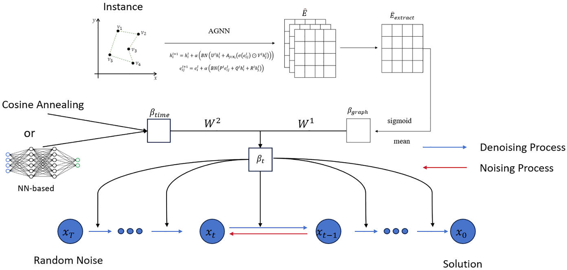
Figure 1: Architecture of the graph-guided noise scheduler in GGDS. Node and edge features of the input instance are processed by an AGNN to yield the enriched edge matrix E^, from which βgraph is extracted via mean-pooling and sigmoid activation. A timestep scheduler (cosine or NN-based) provides βtime, and the two components are linearly fused with weights W1 and W2 to produce the dynamic noise intensity βt that drives both the forward noising and reverse denoising processes of the diffusion solver

Subsequently, a global structural representation is extracted from the edge feature matrix output by the final layer. After applying mean pooling and a Sigmoid activation function, the noise intensity parameter βgraph, which is associated with the graph structure, is generated.

In parallel, the model adopts a predefined noise scheduling strategy along the time dimension (such as cosine annealing or a neural network parameterized approach) to generate time-step-dependent noise intensity βtime. The final noise level βt at each diffusion timestep is obtained by fusing the graph-based and timestep-based components as defined in Eq. (14), which dynamically regulates the noise injection throughout the denoising process.

In both continuous and discrete diffusion models, during the forward noise process, data is progressively noised by polynomial noise until, at the final time step T, the original structure of the data is almost entirely replaced by noise. At this point, the data xT converges to either a normal or uniform distribution, depending on the type of diffusion model used. To ensure that the data follows the expected noise distribution during this process, we design a prior loss Lprior based on standard techniques [40]:

Lprior(x)=Eq(xT|x0)[DKL(q(xT|x0)‖Nt)](15)

where Nt represents the target noise distribution at time step t, which may be either normal or uniform, depending on the chosen diffusion model. With respect to the reconstruction loss mentioned above, the final total loss to be optimized is expressed as:

Ltotal=Lreconstruction+Lprior(x)=E[−log⁡pθ(x0)]+Lprior(x)≤Eq(x1:T|x0)[∑t>1DKL(q(xt−1|xt,x0)||pθ(xt−1|xt))−log⁡pθ(x0|x1)]+Eq(xT|x0)[DKL(q(xT|x0)‖Nt)]+C(16)

where C denotes a constant.

4  Experimental Results

All experiments were conducted on an NVIDIA GeForce RTX 3090 GPU. The proposed method was implemented in PyCharm using Python 3.7, with PyTorch 1.11.0 + cu113 as the deep-learning framework. We evaluated our approach on 2D Euclidean TSP instances generated by uniformly sampling node coordinates in the unit square.

4.1 Experimental Settings

We conducted experiments on problems of varying scales, including TSP-50, TSP-100, and TSP-500. The reference solutions for the training instances of TSP-50 and TSP-100 were provided by Concorde [43], while the training instances for TSP-500 were generated and labeled using the LKH-3 heuristic solver [44]. The test sets for TSP-50 and TSP-100 are sourced from [7,9], containing a total of 1500 instances, while the test set for TSP-500 consists of 128 instances. Following previous work [7,9,38], we measure the differences between models using the following metrics: (1) average path length: the average length of the predicted paths for each instance in the test set (unitless, as coordinates are normalized to the unit square). (2) average performance gap: the average relative performance degradation compared to the benchmark methods (such as Concorde/LKH). (3) average computation time: the average time required to solve each instance in the test set. The comparison includes methods such as AM [7], GCN [9], POMO [22], and DIFUSCO [14], which are among the leading approaches in recent benchmark studies. Additionally, classical heuristic and exact baselines are incorporated for comprehensive evaluation: Concorde [43] and Gurobi [45] serve as exact solvers, LKH-3 [44] as a high-performance heuristic, and Farthest Insertion and 2-OPT [46] as traditional construction and improvement heuristics, respectively. These classical methods provide essential references for assessing both solution quality and computational efficiency across different problem scales.

In all experiments, the denoising step of GGDS is set to T = 1000. Except for the cosine noise schedule and the NN-based noise schedule, we use the combined noise schedule method to set βt (t = 1 to T). The decoding scheme follows previous work [14], with the default decoding strategy being greedy decoding combined with the 2OPT [46] method.

4.2 Main Results

4.2.1 Results for TSP-500

In the experimental results of the discrete GGDS on TSP-500, we compare it with other models as shown in Table 1. In this scale of experiments, the decoding strategies include greedy decoding and sampling decoding (×4), where sampling decoding refers to generating multiple solutions in parallel and selecting the best one. We compare DIFUSCO and GGDS under the same conditions. It is important to note that, except for DIFUSCO and the proposed GGDS variants, the performance data for other baselines (e.g., AM, GCN, POMO) are directly referenced from [11,26]. However, the reported Time values for these models were not measured under the unified hardware environment used in this study. Therefore, these values should be regarded as rough references rather than strict cross-method comparisons.

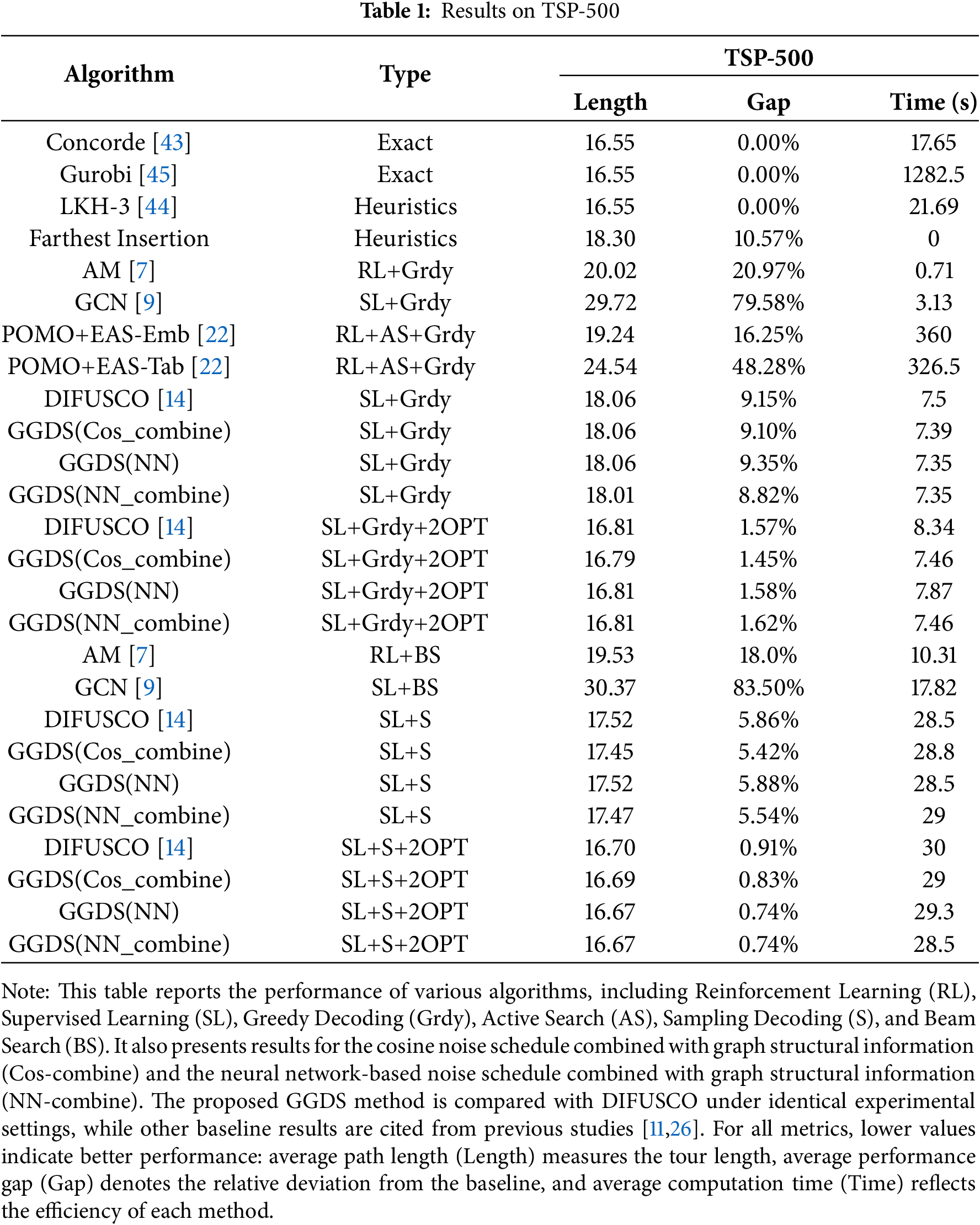
First, in terms of solution quality (Gap), the GGDS method consistently outperforms the existing DIFUSCO [14] approach across multiple settings. Specifically, under the Sampling Decoding + 2OPT configuration, GGDS (NN_combine) and GGDS (Cos_combine) reduce the optimality gap from DIFUSCO [14] 0.91% to 0.74%, corresponding to an 18.7% reduction in the original gap of 0.91%. This demonstrates that incorporating graph structure information to dynamically adjust noise levels can effectively enhance the search ability of diffusion models on complex instances, thereby generating solutions closer to the optimal.

Second, regarding computational efficiency (Time), the GGDS method achieves performance improvements without significant overhead. For instance, under the Sampling Decoding + 2OPT setting, GGDS (Cos_combine) requires an average of 29 s, comparable to DIFUSCO [14] 30 s, and even slightly faster in some configurations (e.g., 28.5 s for GGDS (NN_combine)). This indicates that the proposed graph-guided noise scheduling mechanism improves model performance while maintaining high efficiency, making it practical for solving medium-scale problems.

In the greedy decoding mode, the GGDS method also shows a certain degree of competitiveness. Although its solution quality is slightly inferior to that achieved by the sampling decoding strategy, it offers a significant advantage in runtime (approximately 7.3–7.5 s), making it more suitable for scenarios where solution speed is critical. Notably, GGDS (NN_combine) achieves a Gap of 8.82% under greedy decoding, outperforming DIFUSCO [14] with 9.15%, with nearly identical computation times. This further validates the effectiveness of incorporating graph structure information in lightweight decoding strategies.

In summary, the GGDS method achieves dual improvements in both solution quality and computational efficiency on TSP-500, particularly under the Sampling Decoding + 2OPT configuration, where it demonstrates superior overall performance compared to existing diffusion-based models. The proposed graph-guided noise scheduling mechanism not only improves solution quality but also maintains high efficiency, highlighting its potential and practical value in solving large-scale combinatorial optimization problems. Based on the experimental results of TSP-500, GGDS not only maintains the original solving time but also improves solution quality, validating its applicability in large-scale scenarios.

4.2.2 Results for TSP-50/100

Table 2 compares the performance of the discrete GGDS with other models on the TSP-50 and TSP-100 instances. As shown in previous work [14], DIFUSCO has demonstrated that a sampling decoding strategy achieves excellent results on TSP-50 and TSP-100 instances. However, it is important to note that TSP-50 and TSP-100 are small-scale problems, and their runtime is typically very short (usually in the millisecond range). Therefore, time differences between methods at these scales are not significant. For this reason, we report runtime only for the TSP-500 experiments to reflect the trade-off between efficiency and accuracy. For TSP-50/100, the focus is on solution quality, consistent with previous works like DIFUSCO [14].

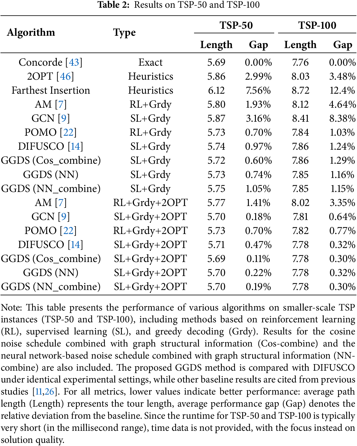
Table 2 shows that although the improvement of GGDS on TSP-50 and TSP-100 is smaller compared to TSP-500, it still follows a consistent trend. On TSP-50, GGDS(Cos_combine) with SL+Grdy decoding reduces the gap from 0.97% (DIFUSCO [14]) to 0.60%, a 38% reduction. With SL+Grdy+2OPT, the gap narrows further to 0.11%, which is only 23% of the 0.47% gap from DIFUSCO [14]. For TSP-100, GGDS(Cos_combine) under SL+Grdy achieves a gap of 1.29%, slightly higher than the 1.24% from DIFUSCO [14]. However, with SL+Grdy+2OPT, both GGDS(Cos_combine) and GGDS(NN_combine) converge to 0.30%, which is lower than the 0.32% of DIFUSCO [14], maintaining a slight advantage. Notably, the NN-based noise schedule performs slightly worse than the Cosine noise schedule when the graph structure is not incorporated, suggesting that the cosine-based graph fusion strategy is more robust than the pure NN-based scheduling in small-scale scenarios. Overall, GGDS shows consistent improvements on TSP-50/100, with results that are “no worse than, and occasionally outperforming” the comparison methods, and its trend aligns with that of TSP-500, verifying the generalization capability of graph-guided noise scheduling across different problem scales.

4.3 Analysis of Algorithm Performance, Weight Sensitivity, and Efficiency

4.3.1 Sensitivity Analysis of W1 and W2 in Noise Scheduling

In this section, we investigate the sensitivity of the proposed GGDS to the weighting coefficients W1 and W2, which control the contribution of βgraph and βtime in the final noise schedule βt (see Eq. (14)). These two hyperparameters are critical as they directly influence the balance between structure-aware and temporally smooth noise injection during the diffusion process.

We conduct a grid search over different combinations of W1 and W2 under the constraint W1+W2<1 and W1+W2→1. All experiments are conducted on the TSP-50 dataset using the SL + Grdy + 2OPT decoding pipeline, following the same training and inference protocol as described in Section 4.1. The denoising step is fixed at T = 1000, and all other architectural hyperparameters (e.g., AGNN depth = 12, width = 32) are inherited from DIFUSCO [14] without modification, ensuring a fair and controlled comparison.

As shown in Fig. 2, GGDS achieves the lowest average optimality gap of 0.11% when W1=0.09 and W2=0.9. This configuration allows the model to retain sufficient graph structural awareness while benefiting from the smoothness of the cosine-based temporal schedule. When W1=0 (i.e., no graph guidance), the gap increases to 0.47%, confirming the necessity of incorporating graph structure into the noise schedule. Conversely, excessively high W1 (e.g., 0.5) leads to overfitting to local structure and degraded generalization, as evidenced by the rising gap.

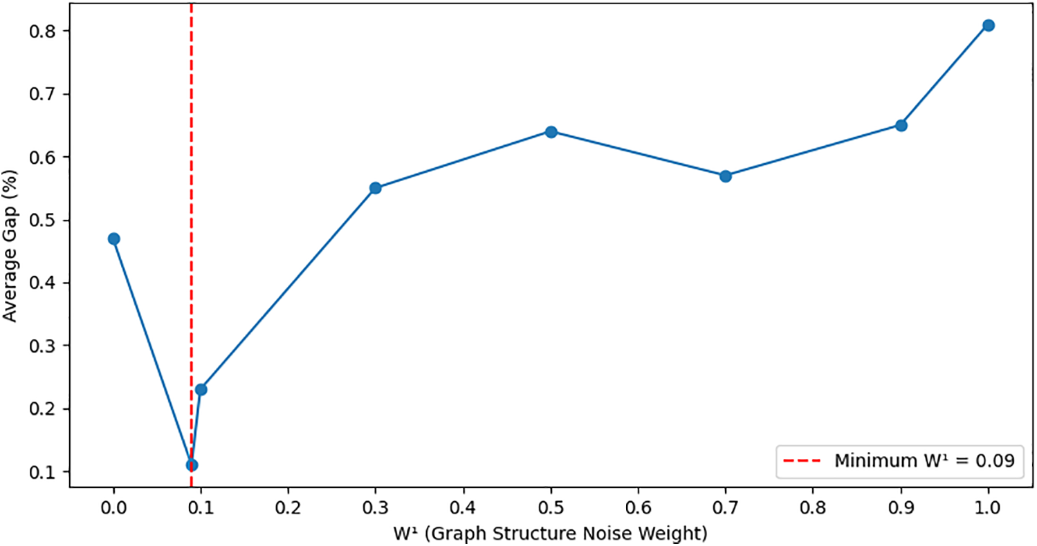
Figure 2: Sensitivity of GGDS optimality gap to graph-structure noise weight W1 on TSP-50. Horizontal axis: W1∈[0,1], controls the relative weight of graph-structure noise; Vertical axis: average gap (%), measures deviation from the optimal tour length. The minimum gap occurs at W1 = 0.09, indicating a balanced injection of graph-aware and temporal noise. Values of W1>0.3 lead to noticeable degradation, confirming that excessive graph-weighting biases the model toward local structure, diminishing solution quality

Notably, the runtime remains stable across all configurations, indicating that the introduction of graph-structure noise adjustment adds negligible computational overhead, consistent with our observations in Section 4.2.

In summary, the weight pair (W1, W2) = (0.09, 0.9) is selected as the default configuration for all subsequent experiments, as it offers the best trade-off between solution quality and efficiency. Unless otherwise specified, this setting is used throughout the paper.

4.3.2 Noise Schedule Effects

Fig. 3 shows the variation in the noise schedule across diffusion timesteps after incorporating instance graph information. The experiments were conducted on TSP-50, with two different noise schedule settings for the diffusion timesteps: cosine annealing noise schedule and NN-based noise schedule. As shown in Fig. 3, after integrating instance graph information, the noise level curve βt becomes smoother. This change suggests that the noise schedule, when combined with graph structure information, effectively adjusts the model’s exploration behavior during the diffusion process, leading to improved performance in solving the TSP problem.

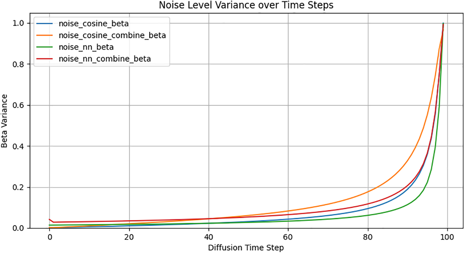
Figure 3: Dynamic variation of noise level βt with diffusion timestep t on TSP-50, Horizontal axis: diffusion timestep t∈ [0, 100]; Vertical axis: noise intensity βt∈ [0, 1]. The solid blue line denotes the standard cosine-annealing schedule, the dashed orange line the purely timestep-based NN schedule, and the solid green and dashed red lines their respective variants fused with graph-structural information. Guided by the graph, the βt trajectory becomes markedly smoother

4.3.3 Evaluation of Algorithm Efficiency

In the diffusion phase, the model employs a 12-layer, 32-width AGNN as the denoising network. The computational cost of a single forward pass is proportional to the number of edges |E| in the graph. Therefore, the total inference time for T diffusion steps is primarily dependent on the number of nodes |V| and the number of diffusion steps T. The computation of graph structure noise, βgraph, is performed through an additional forward pass, contributing negligibly to the overall computation time.

In the decoding phase, GGDS defaults to using a greedy algorithm combined with 2-OPT local search. According to the data in Table 1, for the TSP-500, the average time for GGDS from diffusion step T = 1000 to full decoding is 28.5–29 s, which is comparable to DIFUSCO [14] with a runtime of 30 s. When only the greedy algorithm is used, the runtime drops to 7.3–7.5 s, highlighting the dominant role of diffusion steps in the overall runtime.

In summary, the runtime of GGDS increases approximately linearly with the number of nodes and diffusion steps T. The number of samples introduces a one-time parallelizable overhead. The additional computational cost introduced by the graph-guided noise accounts for less than 3% of the total computation, demonstrating that GGDS has scalability and real-time performance for large-scale problems.

5  Conclusion and Future Work

In this study, we introduce an enhanced method, GGDS, to optimize existing graph-based diffusion models, thereby improving the solution accuracy for the TSP in CO problems. The key innovation lies in the integration of instance graph structure information when generating noise levels. Experimental results demonstrate that this improvement significantly boosts the quality of solutions for TSP problems, reducing the average optimality gap by 18.7% on TSP-500, 6.3% on TSP-100, and 88.7% on TSP-50 compared with the previous best results. We also compare two approaches for generating noise levels across timesteps: one based on cosine annealing and the other using a NN. The performance of these methods varies depending on the problem scale.

However, while GGDS achieves notable improvements in solution quality for TSP instances, it also faces certain limitations. Although experimental results suggest that the integration of GNNs for dynamic noise scheduling does not introduce significant additional overhead in medium-scale problems like TSP-500, the inherent complexity of GNN-based adaptive mechanisms inevitably increases computational demands, particularly as problem scales grow. This may still constrain the practical applicability of GGDS to very large-scale instances without further architectural or algorithmic optimization. Moreover, the current reliance on empirical weight tuning for graph-structure noise and the necessity of post-processing techniques like 2OPT to ensure solution feasibility highlight areas where the method could be further refined. Addressing these issues through more efficient architectures and integrated constraint handling will be crucial for extending the method’s utility to broader and larger problem contexts.

Acknowledgement: None.

Funding Statement: This work was partially supported by the National Science and Technology Council, Taiwan, under grant no. NSTC 114-2221-E-197-005-MY3.

Author Contributions: The authors confirm contribution to the paper as follows: Conceptualization, Yan Kong and Xinpeng Guo; methodology, Yan Kong and Xinpeng Guo; software, Xinpeng Guo; validation, Yan Kong and Chih-Hsien Hsia; formal analysis, Yan Kong and Xinpeng Guo; investigation, Xinpeng Guo and Chih-Hsien Hsia; resources, Chih-Hsien Hsia; data curation, Xinpeng Guo; writing—original draft preparation, Xinpeng Guo; writing—review and editing, Yan Kong and Chih-Hsien Hsia; visualization, Chih-Hsien Hsia; supervision, Yan Kong and Chih-Hsien Hsia; project administration, Chih-Hsien Hsia; funding acquisition, Chih-Hsien Hsia. All authors reviewed the results and approved the final version of the manuscript.

Availability of Data and Materials: Not applicable.

Ethics Approval: Not applicable.

Conflicts of Interest: The authors declare no conflicts of interest to report regarding the present study.

References

1. Hoffman KL. Combinatorial optimization: current successes and directions for the future. J Comput Appl Math. 2000;124(1–2):341–60. [Google Scholar]

2. Tatavarthy SR, Sampangi G. Solving a reverse supply chain TSP by genetic algorithm. Appl Mech Mater. 2015;813:1203–7. doi:10.4028/www.scientific.net/amm.813-814.1203. [Google Scholar] [CrossRef]

3. Stevanovic J, Stevanovic A, Martin PT, Bauer T. Stochastic optimization of traffic control and transit priority settings in VISSIM. Transp Res Part C Emerg Technol. 2008;16(3):332–49. doi:10.1016/j.trc.2008.01.002. [Google Scholar] [CrossRef]

4. Pop PC, Cosma O, Sabo C, Sitar CP. A comprehensive survey on the generalized traveling salesman problem. Eur J Oper Res. 2024;314(3):819–35. doi:10.1016/j.ejor.2023.07.022. [Google Scholar] [CrossRef]

5. Cheikhrouhou O, Khoufi I. A comprehensive survey on the Multiple Traveling Salesman Problem: applications, approaches and taxonomy. Comput Sci Rev. 2021;40(4):100369. doi:10.1016/j.cosrev.2021.100369. [Google Scholar] [CrossRef]

6. Vinyals O, Fortunato M, Jaitly N. Pointer networks. Adv Neural Inf Process Syst. 2015;28:2692–700. doi:10.48550/arXiv.1506.03134. [Google Scholar] [CrossRef]

7. Kool W, Hoof HV, Welling M. Attention, learn to solve routing problems! In: Proceedings of the International Conference on Learning Representations; 2019 May 6–9; New Orleans, LA, USA. p. 7166–90. [cited 2025 Sep 27]. Available from: https://openreview.net/forum?id=ByxBFsRqYm. [Google Scholar]

8. Nowak A, Folqué D, Bruna J. Divide and conquer networks. In: Proceedings of the International Conference on Learning Representations; 2018 Apr 30–May 3; Vancouver, BC, Canada. p. 542–56. [cited 2025 Sep 27]. Available from: https://openreview.net/forum?id=B1jscMbAW. [Google Scholar]

9. Joshi CK, Laurent T, Bresson X. An efficient graph convolutional network technique for the travelling salesman problem. arXiv:1906.01227. 2019. [Google Scholar]

10. Karalias N, Loukas A. Erdos goes neural: an unsupervised learning framework for combinatorial optimization on graphs. Adv Neural Inf Process Syst. 2020;33:6659–72. doi:10.48550/arXiv.2006.10643. [Google Scholar] [CrossRef]

11. Qiu R, Sun Z, Yang Y. Dimes: a differentiable meta solver for combinatorial optimization problems. Adv Neural Inf Process Syst. 2022;35:25531–46. [cited 2025 Sep 27]. Available from: https://arxiv.org/abs/2210.04123. [Google Scholar]

12. Kirkpatrick S, Gelatt CDJr, Vecchi MP. Optimization by simulated annealing. Science. 1983;220(4598):671–80. doi:10.1126/science.220.4598.671. [Google Scholar] [PubMed] [CrossRef]

13. Wu Y, Song W, Cao Z, Zhang J, Lim A. Learning improvement heuristics for solving routing problems. IEEE Trans Neural Netw Learn Syst. 2021;33(9):5057–69. doi:10.1109/tnnls.2021.3068828. [Google Scholar] [PubMed] [CrossRef]

14. Sun Z, Yang Y. Difusco: graph-based diffusion solvers for combinatorial optimization. Adv Neural Inf Process Syst. 2023;36:3706–31. doi:10.1007/978-1-4614-6624-6_97-1. [Google Scholar] [CrossRef]

15. Harshvardhan G, Gourisaria MK, Pandey M, Rautaray SS. A comprehensive survey and analysis of generative models in machine learning. Comput Sci Rev. 2020;38:100285. doi:10.1016/j.cosrev.2020.100285. [Google Scholar] [CrossRef]

16. Iqbal T, Qureshi S. The survey: text generation models in deep learning. J King Saud Univ-Comput Inf Sci. 2022;34(6):2515–28. doi:10.1016/j.jksuci.2020.04.001. [Google Scholar] [CrossRef]

17. Yang L, Zhang Z, Song Y, Hong S, Xu R, Zhao Y, et al. Diffusion models: a comprehensive survey of methods and applications. ACM Comput Surv. 2023;56(4):1–39. doi:10.1145/3626235. [Google Scholar] [CrossRef]

18. Chen T. On the importance of noise scheduling for diffusion models. arXiv:2301.10972. 2023. [Google Scholar]

19. Fan J, Vuaille L, Bäck T, Wang H. On the noise scheduling for generating plausible designs with Diffusion Models. arXiv:2311.11207. 2023. [Google Scholar]

20. Kingma D, Salimans T, Poole B, Ho J. Variational diffusion models. Adv Neural Inf Process Syst. 2021;34:21696–707. doi:10.48550/arXiv.2107.00630. [Google Scholar] [CrossRef]

21. Bello I, Pham H, Le QV, Norouzi M, Bengio S. Neural combinatorial optimization with reinforcement learning. arXiv:1611.09940. 2016. [Google Scholar]

22. Kwon Y-D, Choo J, Kim B, Yoon I, Gwon Y, Min S. Pomo: policy optimization with multiple optima for reinforcement learning. Adv Neural Inf Process Syst. 2020;33:21188–98. doi:10.48550/arXiv.2010.16011. [Google Scholar] [CrossRef]

23. Pan X, Jin Y, Ding Y, Feng M, Zhao L, Song L, et al. H-tsp: hierarchically solving the large-scale traveling salesman problem. Proc AAAI Conf Artif Intell. 2023;2023:9345–53. doi:10.1609/aaai.v37i8.26120. [Google Scholar] [CrossRef]

24. Asani EO, Okeyinka AE, Ajagbe SA, Adebiyi AA, Ogundokun RO, Adekunle TS, et al. A novel insertion solution for the travelling salesman problem. Comput Mater Contin. 2024;79(1):1581–97. doi:10.32604/cmc.2024.047898. [Google Scholar] [CrossRef]

25. Xiao Y, Wang D, Li B, Chen H, Pang W, Wu X, et al. Reinforcement learning-based nonautoregressive solver for traveling salesman problems. IEEE Trans Neural Netw Learn Syst. 2025;36(7):13402–16. doi:10.1109/tnnls.2024.3483231. [Google Scholar] [PubMed] [CrossRef]

26. Fu Z-H, Qiu K-B, Zha H. Generalize a small pre-trained model to arbitrarily large tsp instances. Proc AAAI Conf Artif Intell. 2021;2021:7474–82. doi:10.1609/aaai.v35i8.16916. [Google Scholar] [CrossRef]

27. Costa PD, Rhuggenaath J, Zhang Y, Akcay A, Kaymak U. Learning 2-opt heuristics for routing problems via deep reinforcement learning. SN Comput Sci. 2021;2(388):1–16. doi:10.1007/s42979-021-00779-2. [Google Scholar] [CrossRef]

28. Rani K, Kumar V. Solving travelling salesman problem using genetic algorithm based on heuristic crossover and mutation operator. Int J Res Eng Technol. 2014;2(2):27–34. [cited 2025 Sep 27]. Available from: https://api.semanticscholar.org/CorpusID:212534020. [Google Scholar]

29. Ahmed ZH, Haron H, Al-Tameem A. Appropriate combination of crossover operator and mutation operator in genetic algorithms for the travelling salesman problem. Comput Mater Contin. 2024;79(2):2399. doi:10.32604/cmc.2024.049704. [Google Scholar] [CrossRef]

30. Hottung A, Bhandari B, Tierney K. Learning a latent search space for routing problems using variational autoencoders. In: Proceedings of the International Conference on Learning Representations; 2021 May 3–7; Virtual. p. 10698–710. doi:10.48550/arXiv.1812.06190. [Google Scholar] [CrossRef]

31. Ho J, Jain A, Abbeel P. Denoising diffusion probabilistic models. Adv Neural Inf Process Syst. 2020;33:6840–51. doi:10.48550/arXiv.2006.11239. [Google Scholar] [CrossRef]

32. Ho J, Salimans T, Gritsenko A, Chan W, Norouzi M, Fleet DJ. Video diffusion models. Adv Neural Inf Process Syst. 2022;35:8633–46. doi:10.48550/arXiv.2204.03458. [Google Scholar] [CrossRef]

33. Blattmann A, Dockhorn T, Kulal S, Mendelevitch D, Kilian M, Lorenz D, et al. Stable video diffusion: scaling latent video diffusion models to large datasets. arXiv:2311.15127. 2023. [Google Scholar]

34. Kong Z, Ping W, Huang J, Zhao K, Catanzaro B. Diffwave: a versatile diffusion model for audio synthesis. arXiv:2009.09761. 2020. [Google Scholar]

35. Chen T, Zhang R, Hinton G. Analog bits: generating discrete data using diffusion models with self-conditioning. arXiv:2208.04202. 2022. [Google Scholar]

36. Gong S, Li M, Feng J, Wu Z, Kong L. Diffuseq: sequence to sequence text generation with diffusion models. arXiv:2210.08933. 2022. [Google Scholar]

37. Du X, Wang C, Zhong R, Yan J. Hubrouter: learning global routing via hub generation and pin-hub connection. Adv Neural Inf Process Syst. 2023;36:78558–79. [Google Scholar]

38. Schuetz MJ, Brubaker JK, Katzgraber HG. Combinatorial optimization with physics-inspired graph neural networks. Intelligence NM. 2022;4(4):367–77. doi:10.1038/s42256-022-00468-6. [Google Scholar] [CrossRef]

39. Papadimitriou CH, Steiglitz K. Combinatorial optimization: algorithms and complexity. Mineola, NY, USA: Courier Corporation; 1998. doi:10.1109/TASSP.1984.1164450. [Google Scholar] [CrossRef]

40. Bresson X, Laurent T. An experimental study of neural networks for variable graphs. In: Proceedings of the Workshop Track International Conference on Learning Representations; 2018 Apr 30–May 3; Vancouver, BC, Canada: ICLR. p. 1–3. [Google Scholar]

41. Lee S, Lee K, Park T. ANT: adaptive noise schedule for time series diffusion models. arXiv:2410.14488. 2024. [Google Scholar]

42. Dong M, Kluger Y. Towards understanding and reducing graph structural noise for GNNs. In: Proceedings of the International Conference on Machine Learning; 2023 Jul 23–29; Honolulu, HI, USA. p. 8202–26. [Google Scholar]

43. Applegate D, Bixby R, Chvátal V, Cook W. Concorde TSP solver [Internet]; 2006 [cited 2025 Sep 27]. Available from: https://www.math.uwaterloo.ca/tsp/concorde/index.html. [Google Scholar]

44. Helsgaun K. An extension of the Lin-Kernighan-Helsgaun TSP solver for constrained traveling salesman and vehicle routing problems. Rosk Rosk Univ. 2017;12:966–80. doi:10.13140/RG.2.2.25569.40807. [Google Scholar] [CrossRef]

45. Gurobi Optimization. Gurobi optimizer reference manual [Internet]; 2020 [cited 2025 Sep 27]. Available from: http://www.gurobi.com. [Google Scholar]

46. Croes GA. A method for solving traveling-salesman problems. Oper Res. 1958;6(6):791–812. doi:10.1287/opre.6.6.791. [Google Scholar] [CrossRef]