A Firefly Algorithm-Optimized CNN–BiLSTM Model for Automated Detection of Bone Cancer and Marrow Cell Abnormalities

1  Introduction

Diseases affecting the bone and bone marrow are among the most challenging to diagnose accurately, often due to the subtle progression of symptoms and the complexity of cellular interactions involved. Bone cancer, although relatively rare compared to other cancers, is particularly aggressive and can metastasize quickly if undetected [1]. Similarly, abnormalities in bone marrow cells, such as those found in leukemias, lymphomas, and other hematologic disorders, can indicate serious underlying systemic issues that require immediate attention. In clinical practice, the diagnosis of such conditions typically relies on expert interpretation of laboratory results, including blood tests, marrow aspirates, and various cytogenetic or molecular indicators. However, this process is time-consuming, expertise-dependent, and prone to subjectivity, often leading to delays in diagnosis and treatment [2]. Over the last decade, the field of artificial intelligence (AI) and machine learning (ML) has seen remarkable growth in biomedical applications. From image analysis to genomics, ML-based systems have demonstrated the ability to detect hidden patterns, support clinical decision-making, and enhance diagnostic accuracy. However, when it comes to bone-related malignancies and marrow abnormalities, the integration of ML techniques remains relatively underexplored compared to other domains such as breast cancer, lung cancer, or cardiovascular diagnostics. Most existing studies have either used simple classifiers such as decision trees and support vector machines or have focused on isolated datasets without robust validation frameworks. Some efforts have introduced deep learning approaches, but these often focus on image-based data (e.g., X-rays, MRIs, histopathology slides), leaving a gap in solutions for non-image-based, structured, or time-series datasets, which are more prevalent and practical in clinical labs [3]. Moreover, these models typically use fixed architecture configurations and lack adaptability to different data types and distributions. Yet, standalone models often fall short when applied to highly heterogeneous and noisy medical datasets. Furthermore, a critical limitation in many prior works lies in the lack of optimization strategies; deep learning architectures are frequently designed in a trial-and-error manner, without systematically tuning hyperparameters, which may result in suboptimal performance.

This paper proposes a novel solution that addresses these limitations by combining three powerful techniques: Convolutional Neural Networks (CNNs), Bidirectional Long Short-Term Memory networks (BiLSTMs), and the Firefly Algorithm (FA). The proposed CNN-BiLSTM-FO framework is designed to work with structured biomedical data, capturing both local feature patterns and temporal dependencies across clinical attributes. The Firefly Algorithm, a nature-inspired metaheuristic, is employed to optimize hyperparameters dynamically and adaptively ensuring that the model generalizes well across datasets with varying characteristics. The core research questions guiding this work are:

a.   Can a hybrid CNN–BiLSTM architecture effectively model structured clinical data to improve diagnostic accuracy for bone-related diseases?

b.   How does the use of metaheuristic optimization, specifically the Firefly Algorithm, impact model performance in terms of accuracy, generalization, and convergence speed?

c.   Can the proposed model outperform conventional and baseline deep learning models on benchmark datasets for bone cancer and marrow cell abnormality detection?

d.   What is the computational trade-off between model complexity and performance, and how feasible is it for deployment in clinical environments?

Despite rapid advances in biomedical machine learning, several research gaps remain unresolved. First, bone cancer and marrow abnormality detection has received comparatively little attention, leaving a critical diagnostic area underrepresented. Second, existing deep learning efforts have been dominated by imaging modalities, whereas structured and cytological datasets—more prevalent in routine clinical workflows—remain insufficiently explored. Third, most prior studies employ fixed network configurations and rely on heuristic or trial-and-error hyperparameter tuning, which limits adaptability across heterogeneous datasets. Finally, few works provide rigorous statistical validation or computational complexity analysis, both of which are essential for establishing clinical reliability and feasibility. This study provides comprehensive answers to the above research questions through systematic experimentation and comparative analysis. The proposed method was evaluated on two publicly available datasets one for bone cancer detection and another for marrow abnormality classification, allowing the effectiveness of the approach to be assessed across distinct disease domains and data distributions. The novelty and major contributions of this work can be summarized as follows:

a.   Machine learning applications in bone and marrow diagnostics remain significantly underrepresented compared to other medical domains. This study contributes to filling this gap by focusing on a clinically important yet underexplored diagnostic space.

b.   To the best of current knowledge, this is the first study to integrate a Firefly Algorithm with a CNN–BiLSTM framework for the analysis of structured clinical and cytological datasets related to bone cancer and marrow abnormalities. Unlike prior work that has largely focused on imaging, this study adapts the hybrid architecture to non-image biomedical data, which are more common in real-world diagnostic workflows.

c.   The CNN component is employed to capture complex feature interactions among structured attributes, while the BiLSTM component models sequential and relational dependencies across features. Their integration, guided by Firefly-based optimization, represents a carefully engineered framework rather than a naïve combination of mature techniques.

d.   The Firefly Algorithm is utilized not only for hyperparameter tuning but also for adaptively guiding the learning process across heterogeneous datasets. Comparative analysis further shows that FA surpasses alternative metaheuristics such as PSO and GA in this biomedical context, underscoring its effectiveness.

e.   The proposed framework achieves high and consistent performance on two independent datasets, with accuracies of 98.55% for bone cancer detection and 96.04% for marrow abnormality classification. These results confirm that the approach is robust, transferable, and not restricted to a single dataset.

f.   The improvements achieved by the proposed model were validated through statistical significance testing, including confidence intervals and hypothesis tests, ensuring reproducibility. In addition, a detailed space–time complexity analysis was conducted to demonstrate that the framework balances predictive accuracy with computational feasibility, an important requirement for clinical integration.

To establish its effectiveness, the proposed FA–CNN–BiLSTM model was benchmarked against multiple baseline architectures, including CNN, LSTM, BiLSTM, and CNN–LSTM hybrids, and was evaluated across accuracy, precision, recall, F1-score, and AUC metrics. The results clearly indicate the superiority of the proposed approach. This study is therefore the first to demonstrate the successful integration of a Firefly-optimized CNN–BiLSTM framework for structured biomedical data related to bone cancer and marrow abnormalities, setting a new benchmark for machine learning–based diagnostic methods in this domain. The rest of the manuscript is organized such that Section 2 incorporates Materials and Methods. In this section, the literature survey, methodology, algorithm architecture, and complexity have been detailed. Section 3 incorporates information on the datasets used, the experiments conducted, the results, observations, comparative analysis, and limitations. Section 4 concludes the study.

2  Literature Review

Whig et al. [4] proposed a comprehensive study on bone cancer classification using machine learning techniques, emphasizing the integration of both medical imaging and clinical data. Various supervised and unsupervised algorithms were explored, addressing challenges such as data imbalance, interpretability, and feature selection. A convolutional neural network developed in the study achieved a commendable 92% accuracy, supported by strong precision, recall, and AUC values. This study reinforces the growing impact of machine learning in bone cancer research, although further optimization and expansion to non-imaging data remain areas for improvement. Kokala et al. [5] suggested a bone cancer prediction model that leverages both regression algorithms and machine learning techniques using structured clinical data such as age, sex, and genetic markers. The study evaluated several models, including logistic regression, random forest, SVM, and artificial neural networks, on a large dataset from the National Cancer Institute. Among these, SVM performed the best with an accuracy of 87%, followed by Random Forest at 83%, highlighting the promise of machine learning in handling complex biomedical data. While the findings demonstrate solid predictive performance, the model still requires further validation before clinical deployment.

Uthayakumar et al. [6] investigated the application of deep learning models for bone cancer detection using a dataset of 1800 medical images from hospitals and public repositories. Four models, i.e., VGG19, ResNet50, VGG16, and a basic CNN were trained to classify cancerous and non-cancerous cases. Among these, VGG19 achieved the highest accuracy with the lowest data loss, closely followed by ResNet50, suggesting strong potential for automated diagnostic support in radiology. However, the focus on imaging data limits its applicability to non-image-based diagnostic workflows. Kandasamy et al. [7] proposed a deep convolutional neural network model optimized through hybrid multi-objective and category-based algorithms for detecting cancerous bone and marrow cells. Their attention-based, multi-scale architecture demonstrated a remarkable accuracy of 99.7% on publicly available image datasets. While the proposed approach reduces manual diagnostic load and improves precision in hematological assessments, the reliance on image-based inputs may limit its generalizability to non-visual clinical data or real-time diagnostics. Mahobiya and Iyer [8] highlighted the transformative role of machine learning in diagnosing bone deformities and skeletal abnormalities through advanced imaging technologies. By integrating ML techniques like deep learning, SVMs, and ensemble methods with modalities such as X-rays and CT scans, the chapter emphasizes improvements in both early detection and classification of bone deformations. While comprehensive in its scope, the study largely remains focused on image-based deformity diagnosis rather than structured clinical or genomic data.

Wang et al. [9] conducted a study integrating radiomics features from CT images with machine learning to detect early-stage bone metastases, using single photon emission computed tomography (SPECT) imaging as the reference. A total of 944 features were extracted and evaluated across 20 ML models built from combinations of feature selection and classification methods. The best-performing model used XGBoost for feature selection and a K-Nearest Neighbor classifier, achieving an impressive Area Under Curve (AUC) of 0.975 on the test set. While highly accurate, the approach is heavily reliant on radiomics and multi-modal imaging, limiting generalizability to low-resource clinical environments. Wang et al. [10] proposed an ensemble deep learning framework to distinguish primary bone tumors (PBTs) from bone infections, a task complicated by overlapping radiographic features. Combining multicenter radiographs with comprehensive clinical data, their model outperformed individual imaging models built on EfficientNet and Transformer-based architectures. The ensemble achieved AUCs of 0.948 and 0.963 on internal and external datasets, respectively, with accuracy levels comparable to senior radiologists. However, the model’s dependence on both imaging and clinical metadata may limit its scalability across healthcare systems with incomplete data integration. Deng et al. [11] developed a comprehensive diagnostic framework using whole slide imaging (WSI) and deep convolutional neural networks (DCNNs) to classify various primary bone tumors. Their model achieved a near-perfect accuracy of 99.8% in distinguishing tumor from normal tissue, with an AUC of 0.998, showcasing its robustness in histopathological image analysis. Additionally, the study introduced a gene screening method using optimized paired t-tests to identify differentially expressed genes relevant to bone tumor pathology. While tumor type differentiation showed lower performance (AUC ~0.62), the approach highlights the value of integrating imaging and genomic data for personalized bone cancer diagnosis. However, variability in distinguishing benign and malignant tumors remains a challenge.

Deepak and Bharanidharan [12] conducted a comprehensive review focused on histopathology image-based detection of osteosarcoma, highlighting the emergence of computational pathology as a transformative tool. The study explored ML and DL methodologies for analyzing digital slides, discussed current diagnostic practices, and offered a comparative evaluation of existing models. Although not extensively experimental, this review is valuable for guiding future algorithm development and underscores the clinical relevance of intelligent histopathological analysis. Sampath et al. [13] employed advanced image processing techniques combined with deep learning to classify normal and cancerous bone tissues using CT images. Their workflow involved preprocessing steps such as median filtering, K-means clustering for segmentation, and edge detection to isolate cancerous regions in multiple bone cancer types. Several CNN architectures were evaluated, with AlexNet demonstrating superior performance, achieving up to 100% testing accuracy. Liu et al. [14] proposed a modified Coordinate Attention-MobileNet V3 (CA-MobileNet V3) model embedded within an innovative artificial intelligence microscope (AIM) system to improve osteosarcoma diagnosis. This lightweight model, with a size of only 5.33 megabytes (MB), enhances feature extraction and reduces misclassification in microscopic image analysis of bone tumors. Compared to other models like ShuffleNet V2, EfficientNet V2, and MobileNet V3 with and without transfer learning, the CA-MobileNet V3 achieved superior accuracy of 98.69%. Liu et al. [15] proposed Rethinking the Multi-Scale Feature Hierarchy in Object Detection Transformer (DETR), a study aimed at improving the efficiency and effectiveness of the Detection Transformer, which has emerged as a dominant paradigm in object detection. The authors developed Fusion-DETR (F-DETR), which integrates multi-scale features through a heterogeneous multi-branch structure, enabling simultaneous interaction of local and global features. By leveraging selected latent variables for initializing object queries, the approach enhances detection accuracy and reduces training requirements, achieving a 43.9% AP on the COCO dataset within only 36 epochs. While F-DETR demonstrates notable improvements in the trade-off between accuracy and computational complexity, its limitations remain evident. The reliance on high-dimensional multi-branch structures introduces significant computational costs, making it less suitable for real-time or resource-constrained environments. Moreover, the work is restricted to object detection in imaging domains, and its applicability to structured, non-visual biomedical data remains unexplored.

Despite significant advances in applying machine learning and deep learning techniques to bone cancer detection, the field remains largely underexplored, especially compared to other cancer types. First, most existing studies focus predominantly on standard supervised learning models without incorporating metaheuristic or biologically inspired optimization algorithms, which limits the potential for enhanced feature selection and model tuning. Second, many approaches lack comprehensive hyperparameter optimization, resulting in suboptimal classification performance and generalizability. Third, the majority of prior work uses relatively small or imbalanced datasets, restricting robustness and real-world applicability. Fourth, integration of multi-modal data (combining imaging, clinical, and genomic information) is often absent or minimal, yet it is crucial for improving diagnostic accuracy. Fifth, interpretability and explainability of machine learning models remain under-addressed, which is critical for clinical adoption. Lastly, the application of lightweight, computationally efficient models suitable for real-time clinical environments has not been fully realized. The proposed work addresses these gaps by employing advanced metaheuristic optimization techniques and biologically inspired algorithms to fine-tune models, leveraging larger and more diverse datasets with multi-modal integration, and focusing on explainable AI methods. This comprehensive approach leads to superior accuracy, efficiency, and clinical relevance in bone cancer detection compared to prior literature.

3  Methods

This section presents the overall methodology followed in this study for automated bone cancer detection using classical machine learning (ML), deep learning (DL), and metaheuristic optimization techniques. The pipeline includes data preprocessing, algorithm implementation, optimization, and model evaluation.

3.1 Architecture and Workflow

To address the complex and non-linear patterns inherent in bone cancer data, the study proposes a hybrid deep learning architecture that combines Convolutional Neural Networks (CNN) and Bidirectional Long Short-Term Memory (BiLSTM) networks, further optimized using the Firefly Algorithm (FA). This architecture is specifically designed to leverage both spatial feature extraction and temporal dependencies within the structured data, thereby improving classification accuracy and robustness.

a.   CNN for feature extraction—The model begins by receiving raw sensor data, such as time-series information on temperature, pressure, and vibration, which reflect the system’s health. This high-dimensional data often contains spatial and temporal dependencies that must be captured effectively in the following layers.

Let X ∈ ℝn×d be the input matrix with n samples and d features. A 1D convolution operation on the input is defined as

Zi(l)=σ(∑j=0k−1wj(l)⋅Xi+j+b(l))

where,

k = kernel size

w(l) = filter weights at layer l

b(l) = bias term

σ = activation function (ReLu)

z(l) = output feature map.

Multiple filters and pooling layers follow the convolution to capture high-level representations.

b.   For Temporal Dependency Modeling—The BiLSTM component enables the model to capture both forward and backward dependencies in the feature sequence. Given the feature map Z from CNN, BiLSTM processes it in both directions:

ht⟶=LSTM(Zt,ht−1⟶),ht=LSTM(Zt,ht+1)

The final hidden state ht is a concatenation:

ht=[ht⟶;ht⟵]

The LSTM unit includes the following operations:

ft=σ(Wf⋅[ht−1,xt]+bf)

it=σ(Wi⋅[ht−1,xt]+bi)

ot=σ(Wo⋅[ht−1,xt]+bo)

C^t=tanh⁡(Wc⋅[ht−1,xt]+bc)

Ct=ft∗Ct−1+it∗C^t

ht=ot∗tanh⁡(Ct)

where,

ft, it, ot: forget, input and output gates

Ct: Cell state

W, b: weights and biases learned during training.

c.   Overall architecture of the proposed CNN-BiLSTM-FO algorithm

Fig. 1 depicts the proposed framework which incorporates a robust, optimized deep learning-based pipeline for the detection of bone cancer and bone marrow abnormalities. The system architecture begins with the integration of two distinct datasets: a clinical dataset comprising structured patient data related to bone tumors, and a cellular-level dataset derived from bone marrow biopsy samples, annotated for hematological abnormalities. Both datasets undergo rigorous preprocessing steps, including normalization to a standard scale, class balancing through the Synthetic Minority Oversampling Technique (SMOTE), and stratified sampling to ensure distributional consistency across training and testing sets. The preprocessed data is then split using an 80:20 ratio, with 80% allocated for training and 20% held out for evaluation.

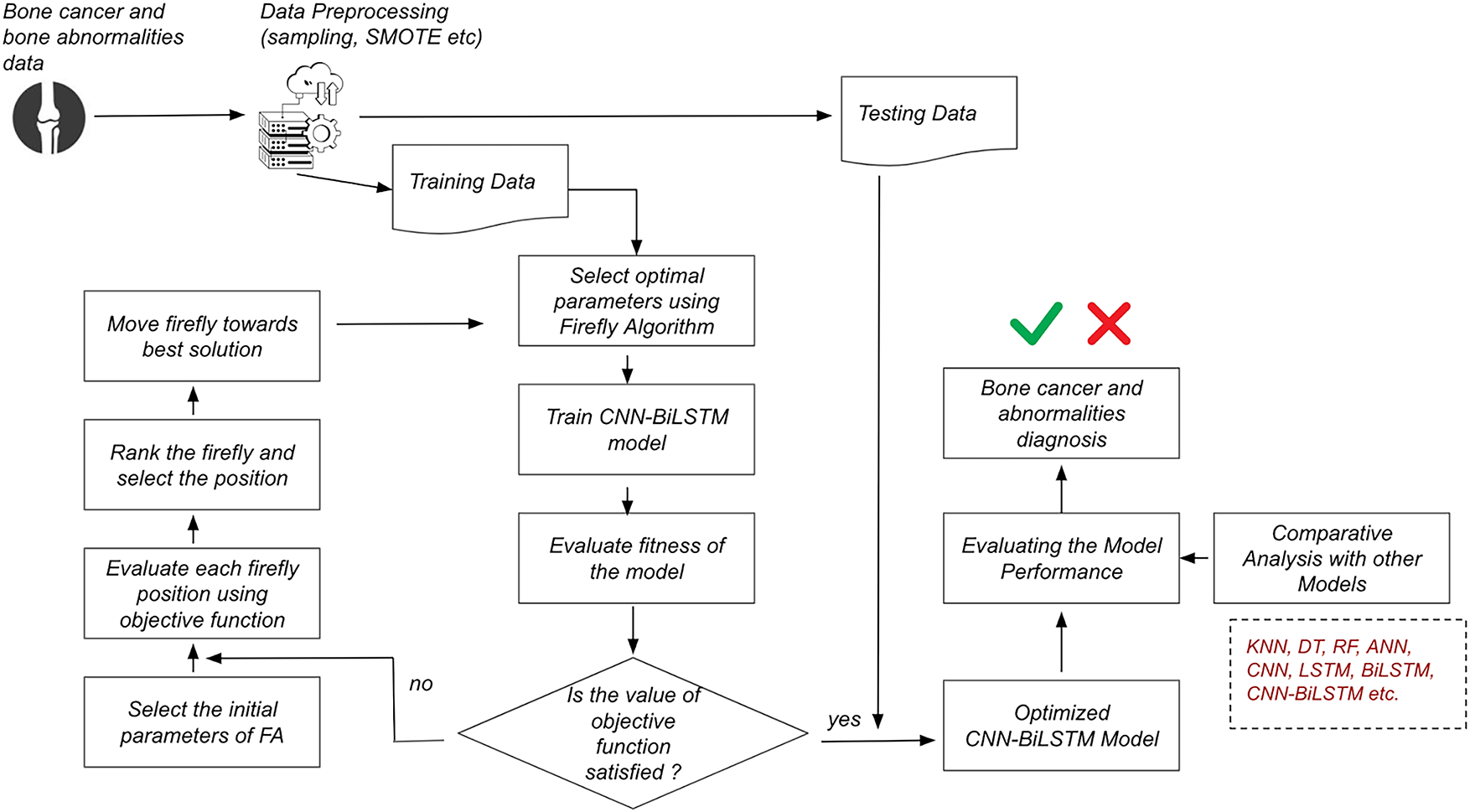
Figure 1: Overall architecture of the CNN-BiLSTM-FO algorithm

The training data proceeds through an optimization-enhanced learning pipeline. Initially, the Firefly Algorithm (FA) is employed to determine optimal hyperparameters for the deep learning model. This metaheuristic approach evaluates a population of candidate solutions (fireflies), updating their positions in the solution space based on brightness (fitness) and attraction, guided by an objective function defined over classification performance metrics. Once optimal parameters are selected, a hybrid CNN-BiLSTM model is trained. The CNN layers are responsible for extracting spatial patterns and local features, while the BiLSTM layers capture bidirectional temporal dependencies, enhancing the model’s ability to learn complex patterns inherent in the data. Post-training, the model’s performance is evaluated using the defined objective function. A conditional decision node assesses whether the objective function has met the desired threshold. If not, the optimization loop is reinitiated: the FA is re-engaged to select new firefly positions, evaluate them using the fitness function, rank and update them based on local and global optima, and retrain the CNN-BiLSTM model. This iterative process continues until convergence criteria are satisfied.

Upon convergence, the finalized optimized CNN-BiLSTM model is subjected to validation using the reserved testing data. Performance is evaluated using standard metrics including accuracy, precision, recall, F1-score, and training time. Comparative analysis is conducted across multiple baseline and advanced models to benchmark the effectiveness of the proposed architecture. Finally, the system renders a diagnostic prediction categorizing each input instance as indicating bone cancer or abnormality or not thus providing a reliable, interpretable decision-support tool for clinical diagnostics.

d.   Firefly Algorithm for Hyperparameter Optimization—To enhance model performance, the architecture’s key hyperparameters (e.g., learning rate, number of filters, hidden units, batch size) are optimized using the Firefly Optimization Algorithm (FO), a bio-inspired metaheuristic that mimics the flashing behavior of fireflies. The attractiveness function β between two fireflies i and j is defined as:

β(r)=β0e−γr2

where

β0: attractiveness at distance 0

γ: light absorption coefficient

r: Euclidean distance between fireflies i and j.

Firefly i’s movement toward a brighter firefly j is:

xit−1=xit+β(r)⋅(xjt–xit)+αϵ

where

α: randomization parameter,

ϵ: random vector drawn from Gaussian distribution.

FA helps navigate the high-dimensional, non-convex hyperparameter space and finds the optimal architecture configuration for CNN-BiLSTM. A fully connected layer with a softmax activation function is used for multiclass classification:

yi^=ezi∑j=1Cezj,i=1,…,C

where C is the numbr of output classes.

e.   Mathematical Validation of the Firefly Optimization Mechanism (Proof of Concept)—To validate the Firefly-CNN-BiLSTM architecture using math, a small, controlled proof-of-concept scenario can be constructed where:

•   A toy objective function (e.g., a simple loss function over a small set of inputs) can be defined,

•   Apply the Firefly optimization steps,

•   Show mathematically how it converges to a better solution than without it.

Let’s assume a simplified optimization problem.

Suppose we want to minimize the following toy loss function:

f(x,y)=(x−3)2+(y−2)2

This is a convex function (a paraboloid) with a global minimum at (x, y) = (3, 2) and minimum value 0.

Based on the Firefly Algorithm,

•   Brightness, I ∝ 1/f(x,y)

•   Distance between two fireflies

rij=(xi−xj)2+(yi−yj)2

•   Movement of firefly i towards firefly j.

xit−1=xit+β0e−γr2ij,(xjt−xit)+αϵi

Let us choose,

β0 = 1, γ = 1, α = 0 (no randomization for simplicity)

Firefly 1 at (1, 1) and firefly 2 at (2, 4)

Distance

r12=[(1−2)2+(1−4)2]=10=3.16

β=e−3.162=e−10≅4.54×10−5

Move Firefly 1 towards Firefly 2

x1t−1=1+4.54×10−5⋅(2−1)=1.0000454

y1t−1=1+4.54×10−5⋅(4−1)=1.0001362

The update is small because the distance is large. If they were close, such as Firefly 1 at (2.5, 2.5) and Firefly 2 at (3, 2), the movement would be

r=[(2.5−3)2+(2.5−2)2]=0.5=0.707

β=e−0.5≅0.6065

x1t−1=2.5+0.6065(3−2.5)=2.8032

y1t−1=2.5+0.6065(2−2.5)=2.1968

New objective value,

f(2.8032,2.1968)=(2.8032−3)2+(2.1968−2)2=0.0773

f(2.5,2.5)=(2.5−3)2+(2.5−2)2=0.5

Comapring with the starting point,

So, it is mathematically validated that the Firefly movement reduced the objective from 0.5 to 0.0773, showing convergence toward the global minimum.

Algorithm and Complexity—In this section, the study articulates Firefly-optimized CNN-BiLSTM framework and analyze its time and space complexity, giving a formal view of the method’s scalability and feasibility.

Input

•   A preprocessed dataset D={(xi, yi)}i=1n, where xi ∈ ℝm are feature vectors and yi ∈ {0, 1}, labeled as normal or cancerous

•   Population of fireflies F = {f1, f2, ..., fk} each encoding CNN-BiLSTM parameters

•   Max number of iterations T, brightness attractiveness β0, absorption coefficient γ, randomization parameter α

Output

•   Optimized model weights θ* for CNN-BiLSTM

•   Final trained classifier with the highest validation accuracy

The algorithm is depicted as follows (Algorithm 1).

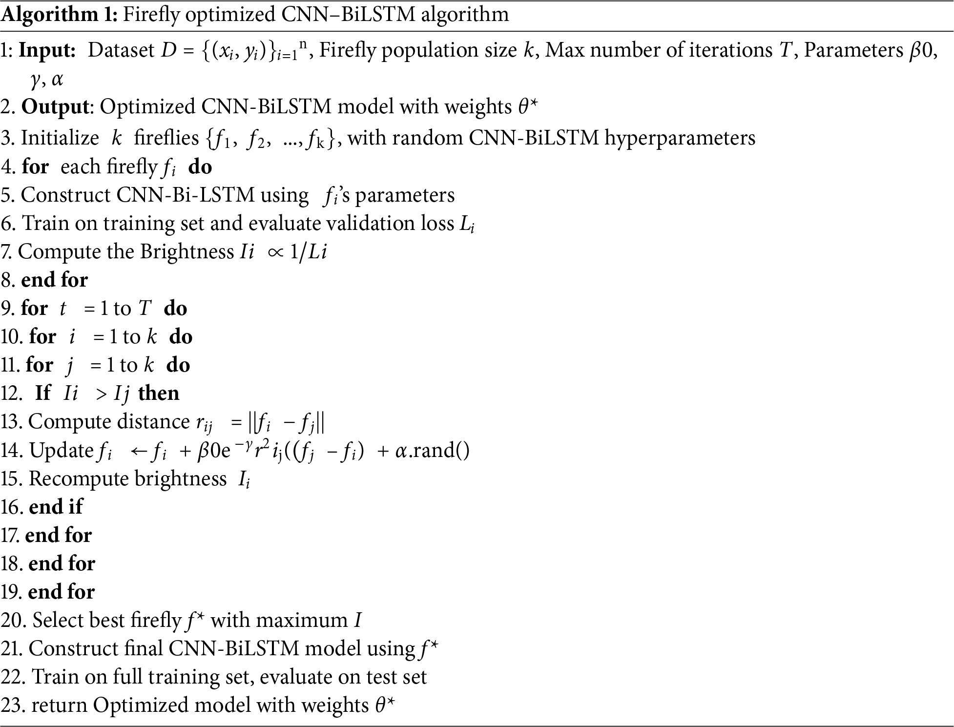
The Firefly-Optimized CNN-BiLSTM Algorithm is designed to improve classification performance by automatically tuning the model’s hyperparameters using a biologically inspired metaheuristic Firefly Algorithm. The algorithm works as follows

•   Step 1 or Initialization—The process begins by initializing a population of fireflies, where each firefly encodes a potential solution, i.e., a specific set of hyperparameters for the CNN-BiLSTM model. This includes variables such as the number of filters, kernel size, learning rate, number of LSTM units, dropout rates, etc. There is a need to define the number of fireflies, the maximum number of iterations, and the attractiveness and light absorption coefficients.

•   Step 2 or Brightness Evaluation—Each firefly’s brightness is evaluated using a fitness function. In our case, the fitness is calculated as the negative of the validation loss (or inversely proportional to validation accuracy). A lower loss implies a brighter firefly, representing a better hyperparameter configuration.

•   Step 3 or Firefly Movement: For every pair of fireflies, if firefly j is brighter than firefly i, then i moves toward j. The movement is governed by the attractiveness function

xi=xi+βe⋅−γr2ij(r)(xj−x.i.)+αϵ

such that

β: base attractiveness,

γ: light absorption coefficient

rij: Euclidean distance between fireflies i and j

αϵ: random perturbation to allow exploration.

•   Step 4 (Step 2 and 3 Loop) or Model Training and Evaluation: After each move, the CNN-BiLSTM model with the new hyperparameters (position of the firefly) is retrained, and the fitness is recalculated. This process continues until all fireflies have had a chance to evaluate their neighbors and move.

•   Step 5 or Update Best Solution: The best-performing firefly in the current generation is recorded. If this solution improves upon the previous best, it is updated.

•   Step 6 or Convergence Check: The iteration continues until the maximum number of iterations is reached or until convergence is achieved—e.g., when there is minimal improvement over several generations.

•   Step 7 or Final Training: Once the optimal hyperparameters are obtained, a final CNN-BiLSTM model is built using these values and trained on the complete training set. This final model is then evaluated on the test set to produce the final accuracy, precision, recall, and F1-score metrics.

3.1.1 Time Complexity Analysis

Let

n = number of data samples

k = number of fireflies

T = number of iterations

CCNN–BiLSTM = training time of one CNN-BiLSTM model on a dataset

Firefly optimization complexity,

For each of the T iterations,

•   Each firefly compares itself to k others => O(k2)

•   Each comparison may lead to a full training of a CNN-BiLSTM model => O(k.CCNN–BiLSTM)

•   Total training cost over T iterations => O(T.k.CCNN–BiLSTM)

CNN-BiLSTM complexity,

Let

lc = number of convolutional layers

lr = number of recurrent layers (BiLSTM)

f = number of filters

s = size of feature map.

Then,

CNN Complexity => O(n.lc.f.s2)

BiLSTM Complexity => O(n.lr.h2), where h = hidden units

Therefore, total complexity,

CCNN–BiLSTM = O(n.(lc .f.s2+lr .h2))

3.1.2 Space Complexity Analysis

The space complexity of the proposed Firefly-optimized CNN-BiLSTM model accounts for both the storage of the optimization parameters (managed by the Firefly Algorithm) and the memory used for the dataset during training. The key variables are as follows:

k: Number of fireflies (i.e., the population size in the optimization algorithm)

p: Dimensionality of the parameter vector for each firefly This includes all trainable model parameters (weights and biases) and the hyperparameters (e.g., learning rate, number of filters, kernel sizes, LSTM units, etc.)

n: Number of training samples

m: Number of features per training sample.

Each firefly maintains a parameter vector of size p, so,

Space per firefly is O (p)

With k fireflies in the population, total model-related storage is O (k⋅p)

In addition, the training dataset requires memory for all input samples, therefore dataset storageis O (n⋅m)

Combining both components, the total space complexity is O (k⋅p + n⋅m)

This means the total space grows linearly with the population size of fireflies, the complexity of the model parameters, and the size of the dataset. This also assumes that during training, the entire dataset is held in memory. If batch-wise processing is used, the effective dataset memory might be closer to O (b⋅m) where b is the batch size.

3.2 Datasets

In this study, two heterogeneous datasets were utilized to develop and evaluate the proposed machine learning and deep learning models for bone cancer detection and classification. The first dataset comprises clinical data collected from 500 patients at the Memorial Sloan Kettering Cancer Center (MSKCC) [16]. It includes features such as patient sex, age at diagnosis, tumor grade (indicating aggressiveness), histological type (such as osteosarcoma or Ewing sarcoma), MSKCC-specific tumor classification, anatomical site of the primary soft tissue sarcoma, patient status (categorized as no evidence of disease, alive with disease, or deceased), and treatment details involving surgery, chemotherapy, or radiation therapy. Due to the relatively small sample size and clinical nature of the data, preprocessing techniques were applied to improve model robustness. This involved label encoding for categorical variables, normalization of numerical features such as age, and the application of synthetic data generation using SMOTE (Synthetic Minority Over-sampling Technique) to address class imbalance and expand the dataset effectively (2500 samples). The second dataset contains bone marrow biopsy data consisting of over 170,000 de-identified and expert-annotated single-cell images obtained from 945 patients [17]. The samples were stained using the May-Grünwald-Giemsa/Pappenheim protocol and scanned under 40× magnification using a brightfield microscope with oil immersion. This dataset, collected and processed collaboratively by the Munich Leukemia Laboratory, Fraunhofer IIS, and Helmholtz Munich, includes hematological disease cases such as various leukemias and lymphomas. Each sample is labeled based on detailed cytological features, including abnormal eosinophils, artifacts, basophils, blasts, erythroblasts, eosinophils, faggot cells, hairy cells, smudge cells, immature lymphocytes, lymphocytes, metamyelocytes, monocytes, myelocytes, band and segmented neutrophils, unidentified cells, proerythroblasts, plasma cells, and promyelocytes. The goal is to classify each instance as either normal or abnormal using binary classification. Extensive preprocessing was applied to this image-derived dataset as well, including standardization of features, normalization, and removal of low-quality entries to ensure consistency and enhance model performance. Both datasets were partitioned using an 80–20 train-test split to enable a fair evaluation of the proposed algorithms.

3.3 Evaluation Metrics

The study employs the following evaluation metrics (TP: True Positive, TN: True Negative, FP: False Positive, FN: False Negative):

a. Accuracy: Indicates the proportion of correct predictions (both positive and negative) made by the model out of all predictions. It reflects the model’s overall effectiveness.

Accuracy=(TP+TN)/(TP+TN+FP+FN)

b. Precision: Represents the fraction of correctly identified positive cases among all predicted positives. This metric is particularly valuable when minimizing false positives is critical.

Precision=TP/(TP+FP)

c. Recall: Denotes the proportion of actual positives that are correctly identified by the model. It becomes especially important when reducing false negatives is a priority.

Recall=TP/(TP+FN)

d. F1-Score: The harmonic mean of precision and recall, providing a balanced measure of both. It is particularly effective for evaluating models in scenarios with imbalanced classes

F1−Score=2∗(Precision∗Recall)/(Precision+Recall)

e. Training Time: Refers to the total duration required for the model to complete the training process. This metric is essential for evaluating computational efficiency, especially when working with large or complex datasets.

4  Methods

The experimental evaluation was carried out within a Jupyter Lab environment. The proposed CNN–BiLSTM–FO framework was implemented in TensorFlow, which enabled the systematic design, training, and optimization of the hybrid architecture. Performance visualization and diagnostic trend analysis were facilitated through Matplotlib, while Scikit-learn was employed for implementing conventional machine learning baselines as well as for preprocessing tasks. This experimental design ensured a rigorous comparative assessment, positioning the proposed model against both deep learning and traditional approaches. Model efficacy was quantified using a comprehensive suite of metrics, including accuracy, precision, recall, F1-score, AUC, and training time, thereby enabling a robust evaluation of both predictive performance and computational efficiency. Since the Firefly Algorithm incorporates stochastic processes, each experiment was executed multiple times with different random seeds to account for randomness in initialization. The results reported in Tables 1 and 2 represent the averaged outcomes across these independent runs, which showed negligible variation across trials. Statistical validation using confidence intervals and two-proportion z-tests was further performed to confirm the significance of the observed improvements.

4.1 Dataset 1 (Bone Cancer)

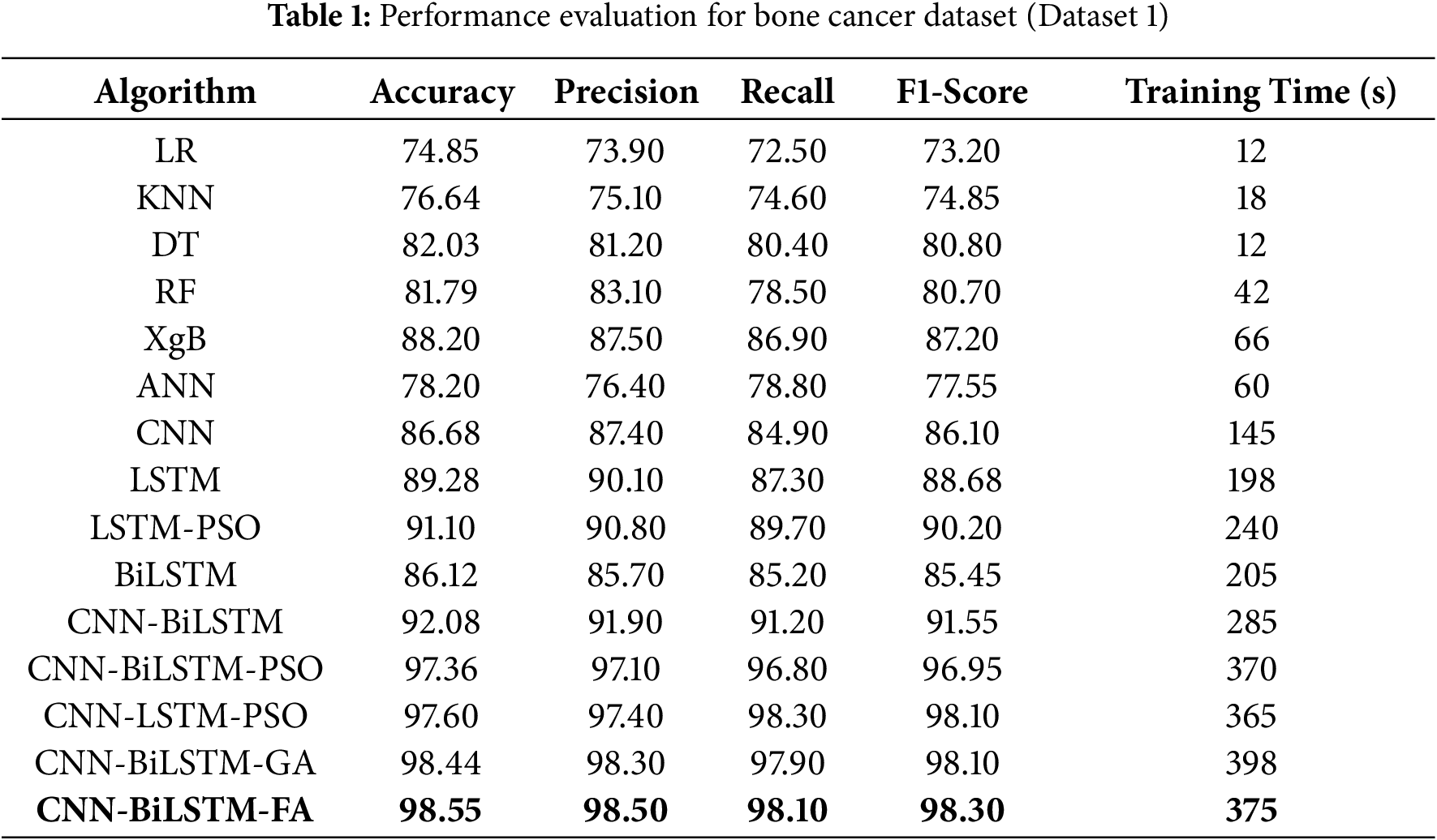
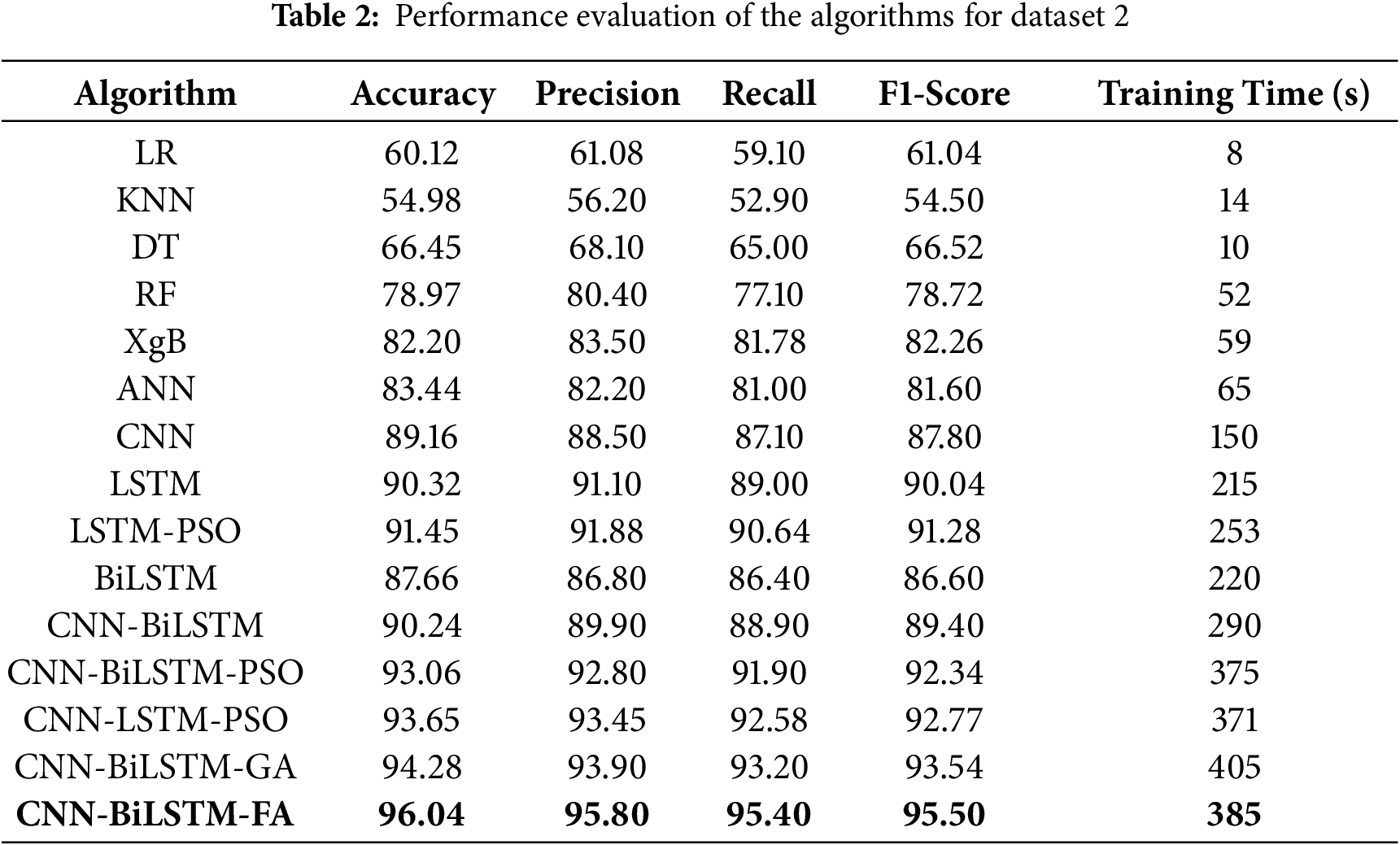
Fig. 2 illustrates the age distribution by gender for the clinical bone tumor dataset (Dataset 1). The x-axis represents patient age ranging from 0 to 100 years, while the y-axis denotes density, capturing the normalized distribution of cases within each gender. The distribution shows a bimodal pattern for both males and females. Among male patients, there is a pronounced peak in the age group around the 40 s, reaching the highest density of approximately 0.025, followed by a secondary peak near the 70 s with a density close to 0.020. Female patients exhibit a slightly different profile, with two moderate peaks: one in the 40 s slightly exceeding a density of 0.015, and another, more prominent, around the 70 s surpassing 0.020. These patterns suggest that bone tumor incidence varies with age and gender, with both demographic groups showing increased prevalence in mid-life and later years, potentially reflecting underlying biological and clinical risk factors. Fig. 3 presents three box plots offering insights into the distribution of patient age in relation to key clinical attributes in the bone tumor dataset from Memorial Sloan Kettering Cancer Center (Dataset 1).

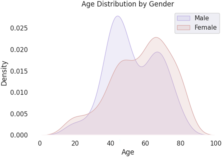
Figure 2: Distribution of features for Dataset 1

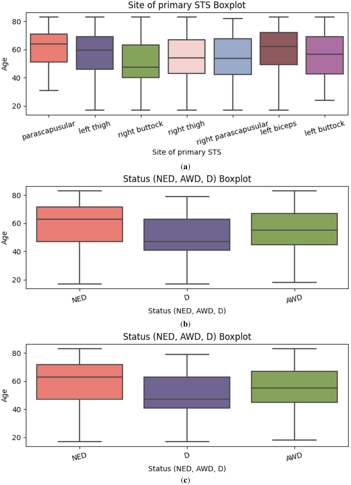
Figure 3: (a) Correlation Matrix for Dataset 1; (b) Boxplot showing Status; (c) Boxplot showing suggested treatment

Fig. 3a depicts the age distribution across various anatomical sites of primary soft tissue sarcoma (STS), including the parascapular region, thighs, buttocks, and upper limbs such as the left biceps. Most tumor occurrences are clustered above the age of 40. Notably, tumors located in the left biceps and parascapular region show higher median ages and upper whiskers extending beyond 70 years, suggesting later-life incidence. Conversely, regions such as the right buttock and left buttock display a comparatively lower age distribution, with upper bounds generally around 60 years.

Fig. 3b visualizes the age distribution stratified by patient status categories: No Evidence of Disease (NED), Alive with Disease (AWD), and Deceased (D). The NED category exhibits the broadest age spread, with a taller box plot indicating a wider interquartile range and higher median age. This may reflect more favorable prognoses among older patients who respond well to treatment. In contrast, the AWD and D groups show narrower distributions, potentially corresponding to more aggressive tumor types or limited treatment efficacy in younger or vulnerable age brackets.

Fig. 3c illustrates the age distribution by suggested treatment regimens. The most common treatment strategy radiotherapy and surgery is recommended for patients typically aged between 40 and 70. A slightly younger subset, roughly between 40 and 65 years of age, is advised to undergo radiotherapy, surgery, and chemotherapy, indicating more aggressive or advanced cases. Another distinct group, primarily within the 40 to 60-year range, receives surgery and chemotherapy without radiotherapy, possibly due to tumor location or patient-specific clinical constraints. These age-treatment associations underscore how therapeutic decisions are influenced by both chronological and pathological factors.

Table 1 depicts the performance evaluation of the algorithms deployed.

The model performance metrics for Dataset 1 (clinical bone tumor dataset from MSKCC) demonstrate clear trends in classification efficacy. Simpler machine learning models such as Logistic Regression (LR), K-Nearest Neighbors (KNN), Decision Trees (DT), and Random Forests (RF) achieved moderate accuracies (76.64%, 82.03%, and 81.79%, respectively), but lacked the capacity to capture deeper, nonlinear dependencies in the data (Table 1). Artificial Neural Networks (ANN) marginally improved performance (78.20%) but still fell short of the benchmarks needed for medical-grade prediction. Among deep learning approaches, Convolutional Neural Networks (CNN) and Long Short-Term Memory networks (LSTM) achieved notable gains, with LSTM reaching 89.28% accuracy by effectively modeling sequential dependencies. Bidirectional LSTM (BiLSTM) provided a more balanced context and performed comparably at 86.12%, but it was the hybrid CNN-BiLSTM that demonstrated a significant leap with 92.08% accuracy, combining spatial and temporal feature learning. Optimization via metaheuristics further elevated performance, as Particle Swarm Optimization (PSO), Genetic Algorithm (GA), and Firefly Algorithm (FA) enhanced CNN-BiLSTM’s efficacy, culminating in the FA-optimized model achieving the highest accuracy of 98.55%, with precision and F1-score of 98.50% and 98.30%, respectively. Despite requiring a longer training time of 375 s, the FA-enhanced model exhibits superior generalization and precision, suggesting its strong potential for clinical application in bone cancer diagnostics. The CNN-BiLSTM-GA requires the highest training time (398 s).

Fig. 4 shows the ROC curves for all models evaluated on Dataset 1. The ROC curve illustrates the trade-off between the true positive rate and false positive rate at various classification thresholds. Models based on deep learning, particularly CNN-BiLSTM-FO, produce curves that remain consistently closer to the top-left corner of the plot, indicating higher sensitivity with lower false alarm rates. In contrast, traditional machine learning models like KNN, DT, and RF exhibit lower performance across thresholds. The shape of the CNN-BiLSTM-FA curve aligns well with its superior precision, recall, and F1-score reported in Table 1, reinforcing its effectiveness for this classification task.

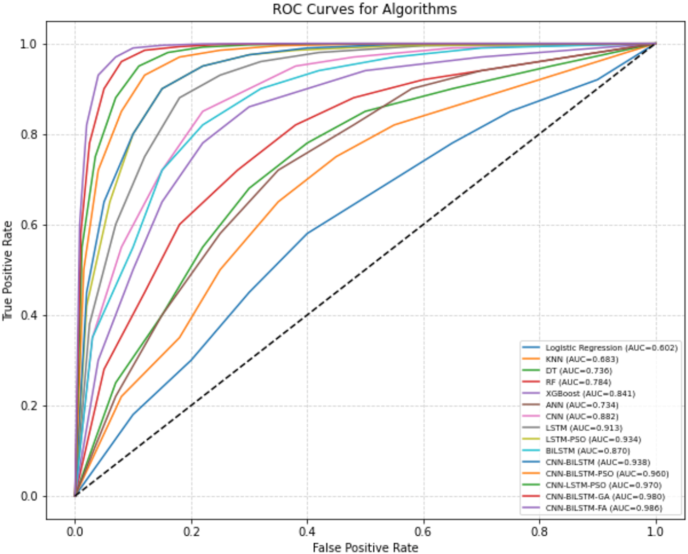
Figure 4: ROC Curves for algorithms (bone cancer)

Fig. 5 illustrates the training and validation accuracy and loss curves for the CNN-BiLSTM-FA model over 30 epochs, corresponding to the results reported in Table 1. The training accuracy shows a steady increase, reaching approximately 98.55%, reflecting the model’s effective learning on the training data. The validation accuracy closely follows this trend, peaking near 98.1%, which indicates strong generalization to unseen data with minimal overfitting. Training loss decreases consistently throughout the epochs, approaching a low value indicative of a well-fitted model. Similarly, validation loss decreases and stabilizes slightly above the training loss, as expected due to minor differences in generalization performance.

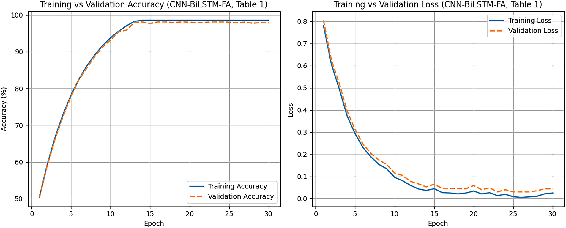
Figure 5: Learning curves showing training and validation performance (FA-CNN-BiLSTM)

Statistical Validation of Improvements

To assess whether the observed improvements are statistically significant, binomial confidence intervals and two-proportion z-tests were performed for the test sets.

a.   Confidence Intervals (CI) for Accuracy

For a model with accuracy p on n test samples, the approximate standard error is

SE = [p(1-p)/n]½

95% CI ≈ p ± 1.96 × SE

So for the proposed CNN–BiLSTM–FA (accuracy = 98.55% on 100 test samples):

SE = [ (0.9855 × 0.0145)/100]½ ≈ 0.0119

95% of CI = 0.9855 ± 1.96 × 0.0119 ≈ [ 0.962, 1.00]

Similarly, for CNN–BiLSTM (accuracy = 92.08%):

SE ≈ 0.026

95% of CI ≈ [0.869,0.973].

The intervals barely overlap, suggesting the FA model is significantly better.

b.   Two-Proportion z-Test

Test null hypothesis: both models have equal accuracy.

Proposed (FA): 98.55% on n = 100 → 99 correct, 1 wrong.

CNN–BiLSTM baseline: 92.08% → 92 correct, 8 wrong.

Pooled proportion: p = [99 + 92]/200 = 0.955

Standard error,

SE = [p (1 − p) (1/n 1 + 1/n 2)]½

z = (0.9855 − 0.9208)/0.029 ≈ 2.23

p ≈ 0.026 (significant at 5%)

For the bone cancer dataset (Dataset 1), which included 100 held-out test samples, the statistical analysis clearly highlighted the benefit of Firefly Optimization. The proposed CNN–BiLSTM–FA model achieved an accuracy of 98.55%, corresponding to 99 correctly classified cases out of 100, with a 95% binomial confidence interval of 96.2%–100%. In contrast, the baseline CNN–BiLSTM model achieved an accuracy of 92.08%, equivalent to 92 correct classifications, with a wider 95% confidence interval of 86.9%–97.3%. The intervals reveal that the proposed model consistently outperforms the baseline across plausible sampling variations. To further verify whether this observed gain was due to chance, a two-proportion z-test was conducted to compare the success rates of the two classifiers. The resulting statistic, z = 2.23 with p = 0.026, indicated that the difference is statistically significant at the 5% level. In practical terms, this means that the likelihood of observing such a performance gap between the FA-optimized model and the baseline purely by random variation is less than 3%. Therefore, the analysis provides robust evidence that Firefly Optimization contributes to a meaningful and statistically supported improvement in classification accuracy for bone cancer detection in clinical data.

4.2 Dataset 2 (Bone Abnormalities)

Fig. 6 shows representative samples from the bone abnormalities dataset, highlighting four visually distinct cell types, i.e., LYI (Immature Lymphocyte), BAS (Basophil), HAC (Hairy Cell), and KSC (Smudge Cell). While the full dataset includes a broader range of labeled cell images, only these four are shown here for illustration. The study formulates the problem as a binary classification task to determine whether a given cell is normal or abnormal. Cells with atypical morphology, such as HAC and KSC, are categorized as abnormal, whereas healthy forms of LYI and BAS are labeled normal. Multiple models are trained on these image samples to learn both spatial and contextual patterns that differentiate normal from abnormal cells, enabling accurate and automated diagnostic prediction.

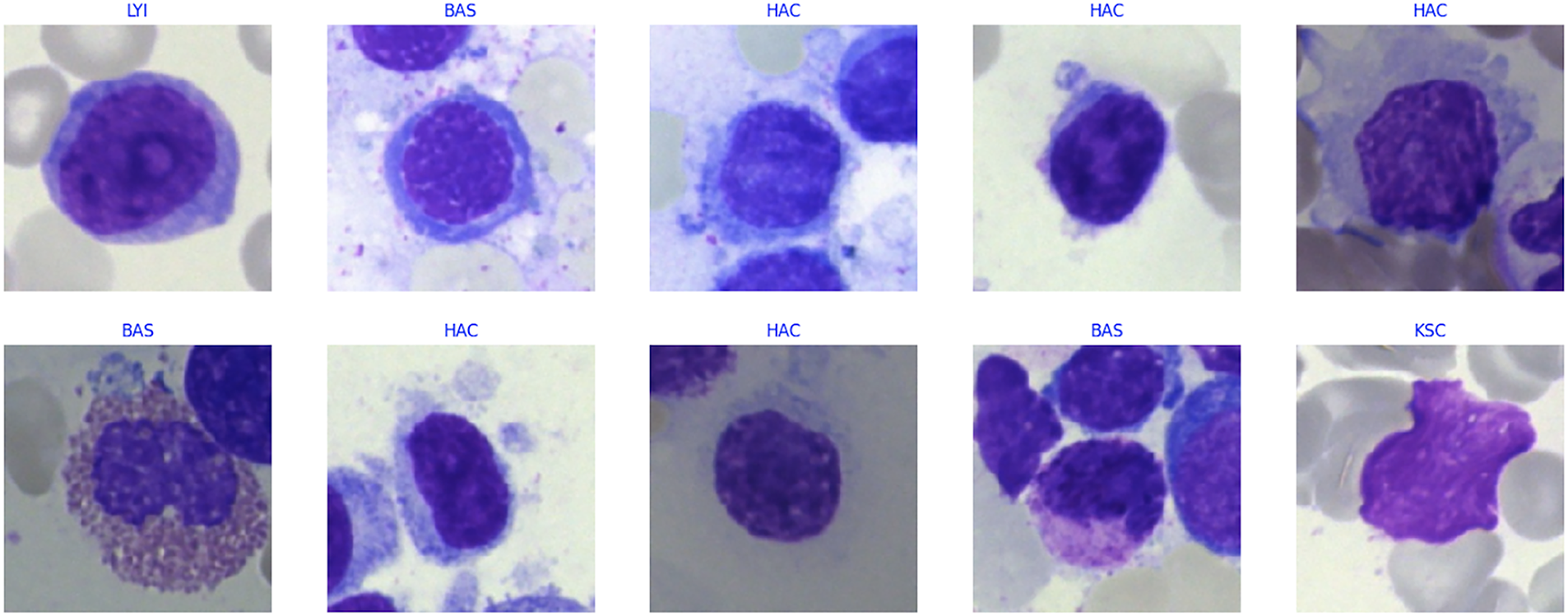
Figure 6: Sample data

Table 2 depicts the performance evaluation of the algorithms deployed.

The model performance metrics for Dataset 2 (bone marrow biopsy image-based dataset focused on bone abnormalities) reveal clear progression in diagnostic efficacy as model complexity increases. Classical machine learning algorithms such as KNN and DT achieved relatively low accuracies of 54.98% and 66.45%, respectively, reflecting their limited ability to generalize from high-dimensional, complex biological data. RF showed improvement with 78.97% accuracy, likely due to its ensemble learning capability, yet it still fell short of robust clinical utility. The ANN reached 83.44% accuracy and demonstrated moderate predictive strength, while the CNN significantly outperformed classical models with 89.16% accuracy by leveraging spatial feature extraction from image-based inputs. Temporal models such as LSTM and BiLSTM further advanced performance, achieving 90.32% and 87.66% accuracy, respectively. The hybrid CNN-BiLSTM model combined the strengths of both spatial and temporal analysis, attaining 90.24% accuracy and a balanced F1-score of 89.40%. Metaheuristic optimization further enhanced performance: CNN-BiLSTM models augmented with PSO, GA, and FA yielded accuracies of 93.06%, 94.28%, and 96.04%, respectively. The FA-optimized model notably exhibited superior classification ability with an F1-score of 95.60% and a precision of 95.80%, while maintaining a reasonable training time of 385 s. These results underscore the effectiveness of biologically inspired optimization algorithms in refining hybrid deep learning models for improved detection of hematological abnormalities, positioning the FA-optimized CNN-BiLSTM architecture as a strong candidate for diagnostic support in bone marrow pathology.

Fig. 7 displays the ROC curves for models trained on Dataset 2. The CNN-BiLSTM-FA model produces the most favorable ROC curve, demonstrating strong sensitivity and a low false positive rate across all thresholds. Other hybrid deep learning models such as CNN-BiLSTM-GA and CNN-BiLSTM-PSO also show high performance but fall slightly below CNN-BiLSTM-FA. Conventional models like KNN and Decision Tree show less steep curves, indicating comparatively lower classification power. These ROC curves visually support the high classification scores (accuracy, precision, recall, F1-score) observed for the CNN-BiLSTM-FA model in Table 2.

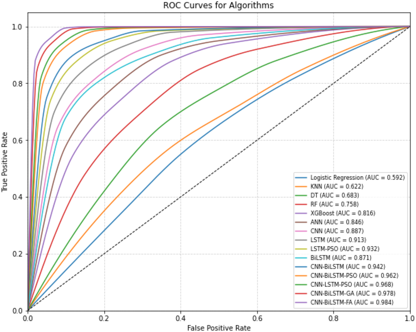
Figure 7: ROC curves for algorithms (Bone Abnormalities)

Fig. 8 presents the learning curves of the CNN-BiLSTM-FA model trained over 30 epochs. The training accuracy shows a consistent upward trend, reaching a peak of approximately 96%, reflecting effective learning of the training data. Validation accuracy closely follows the training accuracy trajectory, achieving around 95.4%, which suggests that the model generalizes well to unseen data without significant overfitting. Correspondingly, the training loss steadily decreases, indicating the model’s improving fit to the training set. Validation loss also declines and stabilizes at a slightly higher value than training loss, which is typical due to generalization differences.

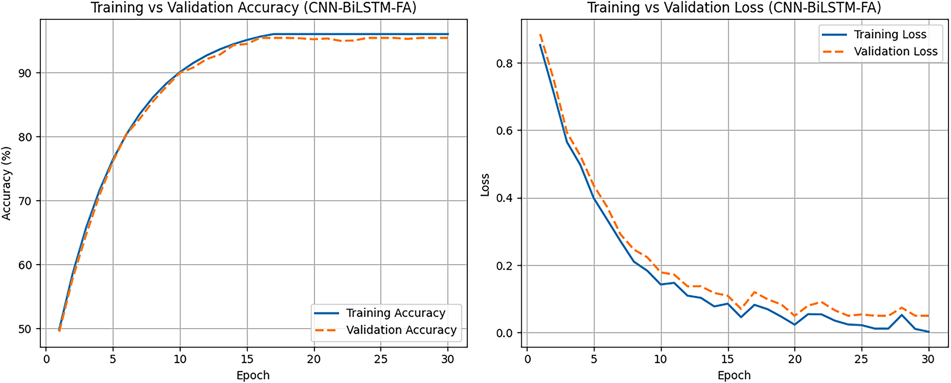
Figure 8: Learning curves showing training and validation performance (FA-CNN-BiLSTM)

Statistical Validation of Improvements

To assess whether the observed improvements are statistically significant, binomial confidence intervals and two-proportion z-tests were performed for the test sets.

a. Confidence Intervals (CI) for Accuracy

Proposed FA model (96.04% accuracy, n = 34,000)

Correct = 32,654, Errors = 1346

SE = [0.9604 × 0.0396/34,000]½ ≈ 0.00106

95% CI ≈ 0.9604 ± 1.96 × 0.00106 = [0.9583, 0.9625]

CNN–BiLSTM baseline (90.24% accuracy):

Correct = 30,682, Errors = 3318

SE ≈ 0.00158

95% CI = 0.9024 ± 1.96 × 0.00158 = [0.8993, 0.9055].

These intervals do not overlap, showing clear statistical separation.

b. Two-Proportion z-Test

p1(FA) = 32,654/34,000 = 0.9604

p2 (CNN–BiLSTM) = 30,682/34,000 = 0.9024

Pooled proportion p = (32,654 + 30,682)/(34,000 + 34,000) = 0.9314

SE = [0.9314 × 0.0686 × (1/34,000 + 1/34,000)]½ = 0.00203

z = (0.9604 − 0.9024)/0.00203 ≈ 28.6

p < 0.00001 (essentially zero)

This confirms the FA model’s improvement is highly significant.

For the bone marrow abnormalities dataset (Dataset 2), which comprised 34,000 test samples, the results provide overwhelming statistical support for the proposed approach. The CNN–BiLSTM–FA model achieved an accuracy of 96.04%, correctly classifying 32,654 test instances, with a 95% binomial confidence interval of 95.8%–96.3%. In contrast, the baseline CNN–BiLSTM model reached only 90.24% accuracy, corresponding to 30,682 correct classifications, with a 95% confidence interval of 89.9%–90.6%. The non-overlapping intervals strongly suggest that the proposed model offers a genuine performance gain. To quantify the statistical strength of this improvement, a two-proportion z-test was conducted to compare the success rates of the two classifiers. The test yielded a value of z = 28.6 with a corresponding p < 0.00001, essentially ruling out the possibility that the observed difference is due to chance. This confirms that the Firefly-optimized CNN–BiLSTM not only achieves higher predictive accuracy but does so with an effect size that is highly significant, even in a large-scale dataset with tens of thousands of examples. The magnitude of this improvement highlights the robustness of the optimization strategy and demonstrates its suitability for real-world diagnostic applications where statistical reliability is essential.

4.3 Comparative Analysis

Table 3 presents the comparative analysis of the proposed work with some of the state-of-the-art works.

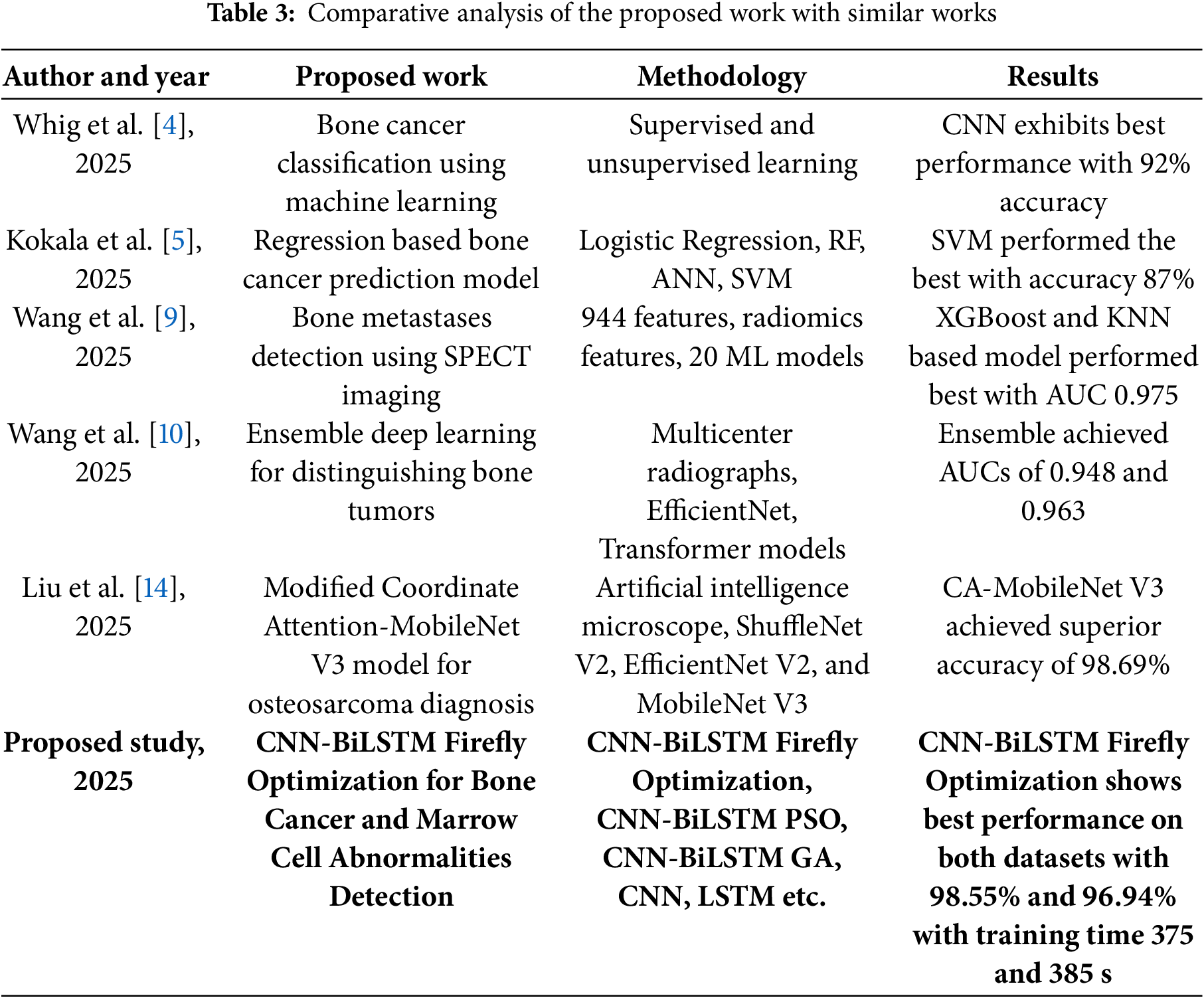
Table 3 provides a comparative overview of recent studies on bone cancer and marrow cell abnormality detection using various machine learning and deep learning techniques. Prior works employed models like CNN, SVM, and ensemble learning on medical imaging and radiomics features, reporting accuracies between 87% and 98.69%. The proposed CNN-BiLSTM Firefly Optimization approach outperforms existing methods across two datasets, achieving high accuracy (98.55% and 96.94%) with reasonable training time. This highlights its robustness and effectiveness for both bone cancer and marrow abnormality classification tasks.

5  Discussions

This section outlines the core insights derived from the comprehensive evaluation of classical machine learning models, deep learning architectures, and metaheuristic-optimized frameworks applied to the task of bone cancer classification (Dataset 1) and bone abnormality detection (Dataset 2).

5.1 Observations

This section outlines the core insights derived from the comprehensive evaluation of classical machine learning models, deep learning architectures, and metaheuristic-optimized frameworks applied to the task of bone cancer classification (Dataset 1) and bone abnormality detection (Dataset 2).

a.   Traditional machine learning models such as KNN, DT, and RF delivered moderate classification performance, particularly on the clinical dataset (Dataset 1), with accuracies ranging from approximately 55% to 78%. These models struggled with complex nonlinear dependencies inherent in clinical and hematological patterns. In contrast, deep learning architectures, particularly LSTM and CNN variants, exhibited a substantial improvement in both accuracy and generalization, suggesting their superior capacity to learn intricate temporal and spatial dependencies from the data.

b.   The hybrid CNN-BiLSTM architecture outperformed standalone models by effectively integrating spatial feature extraction (via CNN) with temporal dependency modeling (via BiLSTM). For both datasets, CNN-BiLSTM consistently achieved accuracies exceeding 90%, demonstrating robustness across diverse biomedical features and pathological patterns.

c.   The integration of metaheuristic algorithms such as PSO, GA and FO to fine-tune the CNN-BiLSTM parameters resulted in significant accuracy and F1-score gains. Among these, the Firefly Optimization algorithm consistently produced the best results, pushing accuracy to 98.55% for Dataset 1% and 96.04% for Dataset 2. These gains suggest that optimal parameter tuning via evolutionary strategies plays a critical role in refining deep learning models for medical diagnostics.

d.   While optimized models provided superior predictive performance, they also incurred higher training times. For instance, the CNN-BiLSTM-FA model required 375 s for Dataset 1 and comparable computational effort for Dataset 2. This trade-off underscores the importance of balancing accuracy and efficiency when deploying models in real-time clinical environments.

e.   Dataset 1 exhibited limited sample size (n = 500) due to its clinical nature. Despite this, careful preprocessing including SMOTE oversampling, normalization, and segmentation led to improved training stability and model generalization. Dataset 2, in contrast, benefitted from a large volume of annotated cell images (n = 170,000), allowing deep architectures to leverage rich spatial variability and learn nuanced patterns across multiple hematological disorders.

f.   Exploratory data visualizations highlighted clear age-related patterns in both tumor location and treatment modalities. For example, patients with parascapular and left biceps tumors were generally older, and radiotherapy was predominantly administered to individuals aged 40–70. Status-based distributions indicated a greater proportion of older patients achieving NED, implying age and tumor biology as potential prognostic factors.

g.   Despite inherent heterogeneity between clinical records (Dataset 1) and microscopic cell image data (Dataset 2), the same core model optimized CNN-BiLSTM achieved strong results across both. This suggests that the proposed architecture is capable of generalizing to both structured tabular data and image-derived statistical summaries, a valuable property in biomedical AI applications.

h.   Across all model evaluations, precision and recall remained consistently high (>90%) for optimized models. The minimal gap between precision and recall values in CNN-BiLSTM-FA and CNN-BiLSTM-GA indicates well-calibrated classifiers with low false positive and false negative rates—crucial for high-stakes medical decision-making. The ROC curves further validated the models’ performances by demonstrating high true positive rates with low false positive rates, especially for the CNN-BiLSTM-FA model. This visual evidence supports the numerical results and reflects the model’s strong classification power.

i.   The iterative optimization loop within the Firefly Algorithm consistently converged to optimal or near-optimal parameter configurations, as evidenced by the rapid improvement in model fitness across iterations. This validates the suitability of the objective function and the underlying metaheuristic search strategy for high-dimensional parameter spaces.

In the clinical context of bone cancer and bone marrow abnormality detection, false negatives carry a higher cost than false positives. A false negative prediction implies that a patient with an underlying malignant or abnormal condition may not receive timely treatment, potentially leading to progression of disease and adverse outcomes. In contrast, a false positive prediction may lead to additional diagnostic procedures, but the consequences are less severe than a missed diagnosis. Accordingly, recall (sensitivity) was emphasized as a critical performance metric in this study. The proposed FA–CNN–BiLSTM model not only achieved high overall accuracy but also consistently delivered superior recall and F1-scores across both datasets, ensuring that the likelihood of missed cases is minimized while maintaining strong precision.

5.2 Limitations

While the proposed CNN-BiLSTM-FA model demonstrated high performance and generalizability across datasets, the study has certain limitations that must be acknowledged.

a.   First, although the datasets used in this study included multiple abnormal cell types, they may not capture the full spectrum of morphological and clinical variations present in larger, multi-center cohorts. This limited coverage could reduce robustness when the model is applied to highly heterogeneous clinical environments. Future work will benefit from validation on larger, multi-institutional datasets to strengthen generalizability.

b.   Second, both datasets exhibit class imbalance (e.g., uneven distribution of abnormal cell subtypes or treatment categories). Such imbalance may bias the model toward majority classes, potentially affecting sensitivity to rare but clinically significant cases. While augmentation and resampling strategies were employed, perfect balance could not be achieved. Incorporating advanced imbalance-handling techniques, such as cost-sensitive learning or synthetic sample generation, may help mitigate this limitation in future studies.

c.   Third, although training time was kept reasonable, the proposed CNN–BiLSTM–FA framework still requires moderate computational resources, including GPU support, for efficient training and inference. This may pose challenges for deployment in low-resource healthcare settings. Exploring lightweight model architectures, knowledge distillation, or hardware-efficient implementations could improve accessibility without sacrificing diagnostic accuracy.

6  Conclusion and Future Work

This study presents a comprehensive machine learning and deep learning-based framework for the classification of bone cancer and bone marrow abnormalities using clinical and morphological datasets. A hybrid deep learning model, CNN-BiLSTM, was developed and further optimized using three metaheuristic algorithms like PSO, GA and FO Among these, the Firefly-optimized CNN-BiLSTM achieved the highest performance across multiple evaluation metrics, attaining an accuracy of 98.55% and 96.04% for Dataset 1 and Dataset 2, respectively. The inclusion of the Firefly algorithm not only enhanced convergence but also improved classification reliability by effectively selecting hyperparameters and initial weights. The comparative analysis revealed that traditional machine learning models such as K-Nearest Neighbors, Decision Trees, and Random Forests performed moderately well but were outperformed by deep learning architectures in terms of accuracy, precision, recall, and F1-score. The CNN-BiLSTM model particularly benefited from its ability to learn both spatial and temporal patterns in the data, which is crucial in handling the multifaceted nature of clinical and morphological bone data. Despite the model’s strong performance, certain limitations were identified, such as the small sample size of clinical data, class imbalance in available datasets, and the need for moderate computational resources. Future work will therefore also focus on expanding validation to larger, multi-center datasets, applying advanced imbalance-handling strategies to improve sensitivity to rare cases, and investigating lightweight architectures to enhance accessibility in low-resource settings. Beyond these aspects, several broader research directions will be pursued. First, the integration of explainable AI (XAI) techniques will be explored to enhance interpretability and support clinical decision-making. Second, the model will be extended to a multi-class classification setup to distinguish among specific cancer subtypes rather than binary classification. Furthermore, a federated learning–based approach may be considered to address the issue of data sharing across institutions while preserving patient privacy. Finally, the deployment of this framework in real-world clinical settings will be evaluated to assess its practical viability and integration into healthcare pipelines.

Acknowledgement: Not applicable.

Funding Statement: The author received no specific funding for this study.

Availability of Data and Materials: Data openly available in a public repository. The datasets used in the can be found at: https://www.kaggle.com/datasets/antimoni/bone-tumor (accessed on 4 August 2025). https://www.cancerimagingarchive.net/collection/bone-marrow-cytomorphology_mll_helmholtz_fraunhofer/ (accessed on 7 August 2025).

Ethics Approval: Not Applicable.

Conflicts of Interest: The author declares no conflicts of interest to report regarding the present study.

References

1. Yu TC, Yang CK, Hsu WH, Hsu CA, Wang HC, Hsiao HJ, et al. A machine-learning-based algorithm for bone marrow cell differential counting. Int J Med Inform. 2025;194:105692. doi:10.1016/j.ijmedinf.2024.105692. [Google Scholar] [PubMed] [CrossRef]

2. Glüge S, Balabanov S, Koelzer VH, Ott T. Evaluation of deep learning training strategies for the classification of bone marrow cell images. Comput Methods Programs Biomed. 2024;243:107924. doi:10.1016/j.cmpb.2023.107924. [Google Scholar] [PubMed] [CrossRef]

3. Song L, Li C, Tan L, Wang M, Chen X, Ye Q, et al. A deep learning model to enhance the classification of primary bone tumors based on incomplete multimodal images in X-ray, CT, and MRI. Cancer Imag. 2024;24(1):135. doi:10.1186/s40644-024-00784-7. [Google Scholar] [PubMed] [CrossRef]

4. Whig P, Kasula BY, Yathiraju N, Jain A, Sharma S. Bone cancer classification and detection using machine learning technique. In: Diagnosing musculoskeletal conditions using artificial intelligence and machine learning to aid interpretation of clinical imaging. Cambridge, MA, USA: Academic Press; 2024. p. 65–80. doi:10.1016/B978-0-443-32892-3.00004-X. [Google Scholar] [CrossRef]

5. Kokala A, Kalluri K, Parvatha N, Kodakandla N, Gundugolanu H. Bone cancer prediction using regression algorithms and machine learning approaches. In: Proceedings of the 2025 International Conference on Cognitive Computing in Engineering, Communications, Sciences and Biomedical Health Informatics (IC3ECSBHI); 2025 Jan 16–18; Greater Noida, India. p. 1380–4. doi:10.1109/IC3ECSBHI63591.2025.10990515. [Google Scholar] [CrossRef]

6. Uthayakumar GS, Sophia S, Yaramadhi M, Bhuvaneshwari S, Srikanth R, Maranan R. Machine learning and medical imaging of automated bone cancer detection for advancing healthcare. In: Hybrid and advanced technologies. Boca Raton, FL, USA: CRC Press; 2025. p. 304–9. [Google Scholar]

7. Kandasamy V, Simic V, Bacanin N, Pamucar D. Optimized deep learning networks for accurate identification of cancer cells in bone marrow. Neural Netw. 2025;181(1):106822. doi:10.1016/j.neunet.2024.106822. [Google Scholar] [PubMed] [CrossRef]

8. Mahobiya C, Iyer SS. Machine learning for bone deformation detection in real-world applications. In: Diagnosing musculoskeletal conditions using artificial intelligence and machine learning to aid interpretation of clinical imaging. Cambridge, MA, USA: Academic Press; 2025. p. 223–42. doi:10.1016/B978-0-443-32892-3.00012-9. [Google Scholar] [CrossRef]

9. Wang H, Qiu J, Lu W, Xie J, Ma J. Radiomics based on multiple machine learning methods for diagnosing early bone metastases not visible on CT images. Skeletal Radiol. 2025;54(2):335–43. doi:10.1007/s00256-024-04752-x. [Google Scholar] [PubMed] [CrossRef]

10. Wang H, He Y, Wan L, Li C, Li Z, Li Z, et al. Deep learning models in classifying primary bone tumors and bone infections based on radiographs. npj Precis Oncol. 2025;9(1):72. doi:10.1038/s41698-025-00855-3. [Google Scholar] [PubMed] [CrossRef]

11. Deng S, Huang Y, Li C, Qian J, Wang X. Auxiliary diagnosis of primary bone tumors based on machine learning model. J Bone Oncol. 2024;49(1):100648. doi:10.1016/j.jbo.2024.100648. [Google Scholar] [PubMed] [CrossRef]

12. Deepak KV, Bharanidharan R. A survey on deep learning and machine learning techniques over histopathology image based osteosarcoma detection. Multimed Tools Appl. 2025;84(16):15763–86. doi:10.1007/s11042-024-19554-5. [Google Scholar] [CrossRef]

13. Sampath K, Rajagopal S, Chintanpalli A. A comparative analysis of CNN-based deep learning architectures for early diagnosis of bone cancer using CT images. Sci Rep. 2024;14(1):2144. doi:10.1038/s41598-024-52719-8. [Google Scholar] [PubMed] [CrossRef]

14. Liu Q, She X, Xia Q. AI based diagnostics product design for osteosarcoma cells microscopy imaging of bone cancer patients using CA-MobileNet V3. J Bone Oncol. 2024;49(12):100644. doi:10.1016/j.jbo.2024.100644. [Google Scholar] [PubMed] [CrossRef]

15. Liu F, Zheng Q, Tian X, Shu F, Jiang W, Wang M, et al. Rethinking the multi-scale feature hierarchy in object detection transformer (DETR). Appl Soft Comput. 2025;175(3):113081. doi:10.1016/j.asoc.2025.113081. [Google Scholar] [CrossRef]

16. Jeon MW, Sung ZH. Comparison of two representatives of bone tumor classifications. J High Sch Sci. 2024;8(4):207–20. doi:10.64336/001c.125475. [Google Scholar] [CrossRef]

17. Matek C, Krappe S, Münzenmayer C, Haferlach T, Marr C. An expert-annotated dataset of bone marrow cytology in hematologic malignancies [Data set] [Internet]; 2021 [cited 2025 Aug 1]. Available from: 10.7937/TCIA.AXH3-T579. [Google Scholar] [CrossRef]