Research on Dynamic Scheduling Method for Hybrid Flow Shop Order Disturbance Based on IMOGWO Algorithm

1  Introduction

The hybrid flow-shop scheduling problem (HFSP), a common type of shop scheduling, integrates traditional permutation flow shop production and parallel machine scheduling. It is widely applied in industries such as steelmaking, casting, chemical engineering, textile, machinery, and assembly [1]. During the manufacturing process of hybrid flow shops, various random factors and dynamic disturbances often exist. As a direct reflection of changes in external market demand, order disturbance is characterized by considerable suddenness and unpredictability [2]. Balancing production efficiency and stability in hybrid flow shops amidst order disturbances holds significant theoretical importance and practical application value. Dynamic scheduling is an anti-interference method for workshops, which replans schemes by integrating the current status, unprocessed tasks, and disturbances [3]. Due to its capability to handle production uncertainties, dynamic scheduling has become a research focus in the HFSP field.

In terms of shop scheduling models, multi-objective optimization is more in line with practical requirements in most cases. Yang et al. [4] constructed a mathematical model with maximum makespan and total delay time as objectives for the dynamic shop scheduling problem. Li et al. [5] addressed dynamic shop scheduling by formulating a model focused on makespan, worker fatigue, and scheduling deviation. Shi et al. [6] developed a mathematical model targeting makespan, total job delay time, overall machine idle time, and total energy use as its objective function for the problem of random job arrivals in the shop. Liu et al. [7] established a mathematical model aiming at minimizing makespan and total energy consumption for the HFSP.

Existing studies on dynamic scheduling strategies mainly focus on event-driven, periodic, and hybrid rescheduling. Wang et al. [8] proposed a hybrid adaptive rescheduling strategy to address uncertain disturbances. Chen et al. [9] adopted event-driven rescheduling to resolve dynamic disturbances in production. Zhu et al. [10] utilized a hybrid rescheduling approach to handle order cancellation disturbances. Wei et al. [11] adopted a hybrid rescheduling strategy to solve the shop scheduling problem with machine failures. Angel-Bello et al. [12] applied a periodic rescheduling strategy to cope with random order arrivals.

Currently, the most commonly used methods for solving HFSP are meta-heuristic algorithms, with swarm intelligence optimization algorithms and genetic algorithms as typical representatives. Zou et al. [13] proposed a multi-level subpopulation-based particle swarm optimization algorithm (MLPSO). Wang et al. [14] developed a variable-representation discrete ABC algorithm. Zeng et al. [15] designed an improved NSGA-III algorithm. The GWO algorithm is a new type of swarm intelligence optimization algorithm inspired by the hunting behavior and internal hierarchical system of wolf packs. This algorithm features a simple basic framework, a small number of parameters, and has been proven to be superior to other heuristic algorithms in terms of convergence and optimization performance [16]. Li et al. [17] designed a reasonable encoding and decoding scheme, developed four crossover operators to expand the search space, and proposed a local search strategy with the concept of key factories, thereby improving the exploitability of the IGWO algorithm. Lin et al. [18] used a reinforcement learning algorithm to optimize the parameters of the GWO algorithm, effectively enhancing the algorithm’s effectiveness. Zheng and Chen [19] developed a Q-learning multi-objective grey wolf optimizer (QMOGWO) algorithm and designed several initialization strategies and local search strategies to address the distributed hybrid flow shop scheduling problem.

Overall, existing studies have conducted a series of discussions on dynamic shop scheduling problems, laying a foundation for the research in this paper, but still need to be expanded. First, regarding the construction of dynamic scheduling models, existing studies have mostly focused on factors such as time and energy consumption, while attention to the stability of scheduling systems remains insufficient. To address this, on the premise of selecting the maximum makespan (reflecting production efficiency) and the delivery time deviation (measuring the satisfaction of customer demands) as static optimization objectives, this paper further introduces the scheme deviation degree (related to the stability of scheduling systems) to construct a dynamic scheduling mathematical model. Second, concerning dynamic scheduling strategies, the lack of an effective driving mechanism may lead to excessive or insufficient rescheduling in actual production processes, which causes adverse effects such as a decrease in the stability of the production line or a lack of rapid response capability. Thus, this paper designs a dynamic scheduling strategy based on the order disturbance degree. Third, regarding solution algorithms, the encircling and hunting mechanism of the GWO algorithm ensures its high accuracy, fast convergence speed, few parameters, and strong optimization ability. Inspired by the algorithm improvements in the preceding literature, this paper designs an IMOGWO algorithm to solve the dynamic HFSP.

The main contributions of this paper are as follows: (1) A multi-objective dynamic scheduling model is constructed. With maximum makespan, delivery time deviation, and scheme deviation degree as the optimization objectives, the model enables rapid response to order disturbances while ensuring the stability of the production system. (2) An adaptive dynamic scheduling strategy based on the order disturbance degree is designed. It adopts different scheduling strategies according to varying degrees of order disturbance, which avoids excessive or insufficient rescheduling frequency in the actual production process of the shop. (3) An IMOGWO algorithm is designed. This algorithm integrates the “job-machine” two-layer encoding strategy, the timing-driven two-stage decoding strategy, the opposition-based learning initialization population strategy, the POX crossover strategy, the dual-operation dynamic mutation strategy, and the variable neighborhood search (VNS) strategy. Experimental results sho w that this algorithm outperforms the existing algorithms commonly used for HFSP.

The structure of this paper is organized as follows: Section 2 provides a detailed description of the problem and proposes a corresponding mathematical model. Section 3 presents an adaptive dynamic scheduling strategy based on the order disturbance degree. Section 4 focuses on algorithm design. Section 5 conducts experimental simulation and case analysis. Section 6 draws the conclusion and outlines future work.

2  Problem Description and Modeling

2.1 Problem Description and Assumptions

The dynamic scheduling problem of the hybrid flow shop studied in this paper can be described as follows: There are n jobs processed through j operations. The set of process stages is S={1,2,⋯,j,⋯,s}. Each stage j contains ej parallel machines, corresponding to the processing machine set Ej, and at least one stage has 2 or more parallel machines. The set of processing equipment is E={1,2,⋯,k,⋯,e}. The initial order W={W1,W2,⋯,Wi,⋯,Wn} includes n types of jobs, where the batch set of jobs Wi is Xi={1,2,⋯,x,⋯,xi}. Wi.x denotes the x-th batch of jobs Wi, and Wij.x represents the processing of jobs Wi.x at stage j. Its optional processing machine set is Eij⊆Ej. On this basis, three types of order disturbance events, namely order expediting, order cancellation, and order insertion, are considered. At a random moment Tr, there exist WI expedited jobs WI={WI,1,WI,2,⋯,WI,i,⋯,WI,n}, WII inserted jobs WII={WII,1,WII,2,⋯,WII,i,⋯,WII,n}, WIII withdrawn jobs WIII={WIII,1,WIII,2,⋯,WIII,i,⋯,WIII,n}. When a disturbance event occurs, different rescheduling schemes are generated according to different situations to minimize the impact of emergencies on production.

Based on the above description, the following assumptions are made in this paper:

(1)   Job production follows the batch production principle, and batch production is carried out according to the optimal batch size.

(2)   There is no sequence constraint between different batches of jobs to realize flexible scheduling.

(3)   The processing of the same batch of jobs cannot be interrupted;

(4)   The preparation time before job processing has been included in the actual processing time.

(5)   All parts can be served directly at the initial moment, and all processing equipment can be used for processing production activities at the initial moment.

(6)   There are infinite buffer storage areas between two consecutive processing operations.

(7)   When implementing the dynamic scheduling strategy, the completed jobs and the jobs in processing are not scheduled.

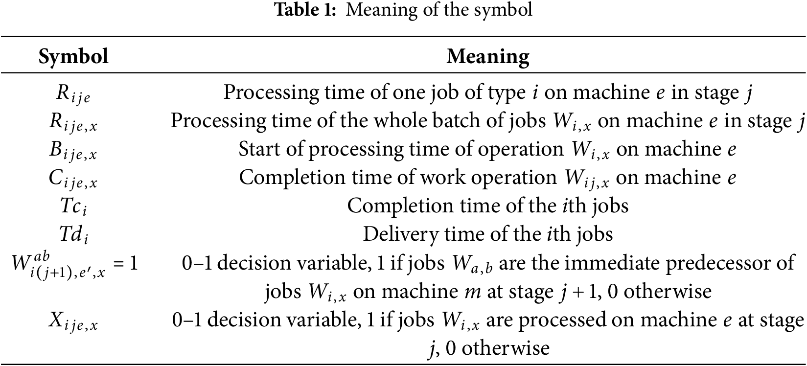
To facilitate modeling, the relevant parameter symbols and their meanings in the model are presented in Table 1.

2.2 Modeling

To address order disturbances and rescheduling problems, this paper divides the scheduling problem into two phases: the first phase is the initial static scheduling before the order disturbance; the second phase is the dynamic optimization rescheduling of all unfinished jobs after the order disturbance.

2.2.1 Static Scheduling Optimization Model

The initial static scheduling problem before order disturbance is modeled to minimize the maximum makespan and minimize the delivery time deviation as the performance optimization objectives, and the objective function is established as shown below:

minf1=max{Cije,x}(1)

minf2=1n∑i=1n(Tdi−Tci)2(2)

The following constraints are established:

∑x=1XiSum(Wi,x)=Sum(Wi)∀i(3)

Rije,x=Rije×Sum(Wi,x)∀i,j,∀x∈{1,2,⋯,Xi},∀e∈Eij(4)

Cije,x=Bije,x+Rije,x,when Xije,x=1,∀i,j,∀x∈Xi,∀e∈Eij(5)

Tci=max{Cije,x},∀j,e,x(6)

Bi(j+1)e′,x=max{Cije,x,Ca(j+1)e′,b},whenXi(j+1)e′,x,Xa(j+1)e′,b,Wi(j+1),e′,xab=1∀i,a,j,∀x∈Xi,∀b∈Xa,∀e∈Eij,∀e′∈Ei(j+1)(7)

∑i=1n∑x=1XiXije,x=1,∀t∈[Bije,x,Cije,x],∀e∈Ej,∀j(8)

∑e∈EjXije,x=1,∀t∈[Bije,x,Cije,x],∀x∈{1,2,⋯,Xi},∀i,j(9)

Rije,Rije,x≥0,∀x∈{1,2,⋯,Xi},∀e∈Eij,∀i,j(10)

Bije,x≥0,∀x∈{1,2,⋯,Xi},∀e∈Eij,∀i,j(11)

Constraints (3) and (4) are time constraints for job batch processing. Constraints (5) and (6) are processing time constraints. Constraint (7) is the mixed flow shop operation sequence constraint. It means that the start time of the next operation of the job is determined by the end time of the previous operation and the processing completion time of the machine where the next operation is performed. Constraints (8) and (9) are machine capacity constraints. It indicates that for any batch of jobs, they can be processed by only one machine in the same time period, and the same machine can process only the same batch of jobs at the same time. Constraint (10) denotes that the processing time of all jobs is positive. Constraint (11) means that all jobs can be processed at moment 0.

2.2.2 Dynamic Scheduling Optimization Model

(1)   Description of order disturbance events

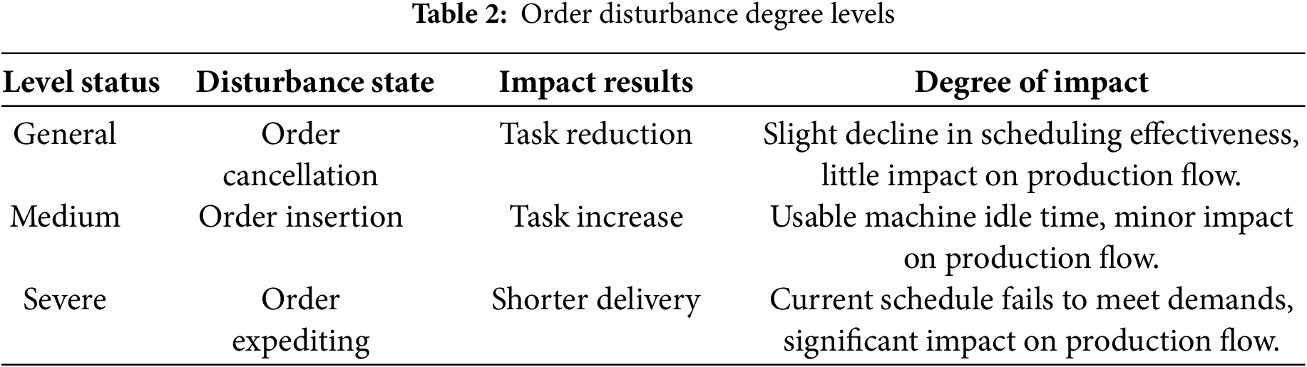
Complete rescheduling after all perturbation events in the production process can detrimentally impact the stability of the production system. Therefore, drawing upon the scheduling characteristics of a hybrid flow shop [20], we have categorized order disturbance events into varying degrees. Dynamic scheduling strategies are matched according to these levels. When the disturbance is minor, partial rescheduling or temporary non-rescheduling can be adopted to stabilize production. The specifics of this categorization are outlined in Table 2.

(2)   Objective functions and constraints

In actual production, various order disturbances can disrupt the originally formulated scheduling plan. To maintain the stability of the scheduling system and reduce adjustment costs, a stability indicator for minimizing the scheme deviation degree (including operation deviation cost and machine deviation cost) is introduced based on the static scheduling model. The constraints remain identical to those in the static scheduling optimization model, with the only modification being that the solution scope is shifted to the set of disturbance orders or the combination of disturbance orders and remaining unfinished jobs. The objective functions are formulated as follows:

minf3=min{∑i=1n∑j=1nipj|Bij′−Bij|+∑e=1kpeye}(12)

Operation Deviation Cost (ODC): When the operation deviation cost fluctuates within a certain range, it significantly impacts the shop’s resource consumption. For example, it may require rescheduling material delivery timings, or even necessitate immediate delivery for certain materials, and so on.

odc=∑i=1n∑j=1nipj|Bij′−Bij|(13)

where n and ni denote the number of unprocessed jobs and operations at the start of dynamic scheduling, respectively. Bij′ and Bij represent the start times of the jth operation for the ith job in the rescheduling scheme and the original static scheduling scheme, respectively. pj is the penalty coefficient associated with changes in the start time of processing at stage j, where pj is set to 1. The calculation of ODC only considers jobs that exist in both the original scheduling plan and the rescheduling scheme.

Machine Deviation Cost (MDC): When an operation is added to or removed from a machine, it inevitably triggers changes in the machine’s tooling or fixtures. This needs consideration of the machine deviation cost.

mdc=∑e=1kpeye(14)

where ye represents the total number of operation changes on machine e at the start of dynamic scheduling compared to the initial scheduling plan. pe is the penalty coefficient of the machine caused by operation changes in rescheduling, where pe is set to 1.

3  Adaptive Dynamic Scheduling Strategy Based on the Order Disturbance Degree

3.1 Dynamic Scheduling Driving Mechanism

Dynamic scheduling driving mechanism, also known as the dynamic scheduling strategy, refers to a mechanism that replans or adjusts the original scheduling plan due to changes or the occurrence of specific events [11]. Currently, it mainly includes periodic scheduling strategy, event-triggered scheduling strategy, and hybrid scheduling strategy [21].

Considering the detrimental impacts of the previously mentioned three strategies, such as excessive or insufficient scheduling times, which may lead to reduced stability of the production line or inadequate rapid response capability, this paper proposes a method integrating the order disturbance degree with the hybrid scheduling strategy, thereby designing an adaptive dynamic scheduling strategy based on the order disturbance degree. The specific steps are as follows: construct a set D of n disrupted jobs, each containing hd operations, and define the makespan of the initial scheduling plan as the current scheduling cycle time. Upon the occurrence of disturbance orders, evaluate the level of the current order disturbance event, and calculate the order disturbance degree S based on the impact level, operation processing time, and delivery date, etc. The detailed procedure is presented in Section 3.3. The order disturbance degree S, the coefficient of delivery date of the disturbed job, and the coefficient of disturbance level are calculated as shown in Eqs. (15)–(17).

S=∑d=1n(αdβd∑k=1hdT¯d,k)T′×100%(15)

βd=1+1LTd,∀d∈D(16)

αd={1.0,General disturbance events1.5,Medium disturbance events2.0,Severe disturbance events,∀d∈D(17)

where αd denotes the disturbance coefficient of the disturbed job d, βd denotes the delivery date coefficient of the disturbed job d, T¯d,k denotes the average processing time of the kth operation of the disturbed job d, T′ denotes the remaining time of the current scheduling cycle, and LTd denotes the delivery date of the disturbed job d.

3.2 Dynamic Scheduling Modes

After determining the dynamic scheduling strategy, it is necessary to determine the dynamic scheduling mode. This paper employs three dynamic scheduling modes based on different scenarios: complete rescheduling, partial rescheduling, and left-shift rescheduling [22].

(1)   Complete rescheduling

After a disturbance occurs, re-optimize the remaining unprocessed jobs and disturbed jobs to ensure the global optimality of the scheduling scheme.

(2)   Partial rescheduling

Only scheduling the disturbed job within the idle time periods of the initial scheme, it maintains a certain degree of similarity to the initial scheduling scheme and exhibits good stability.

(3)   Left-shift rescheduling

Remove the operations of canceled jobs, shift the remaining operations to the left to adjust their start times while retaining the original equipment allocation. This approach maintains a certain degree of similarity to the initial scheduling scheme and is consistent with actual production scenarios.

In production scheduling, the degree of order disturbance S is used as the decision threshold: when S>100\% , the disturbance is judged to exceed the original plan’s capacity, triggering the dynamic scheduling mechanism. This paper only considers one type of disturbance occurring at the same moment. For order cancellation disturbances, directly adopts left-shift rescheduling; for non-cancellation disturbances, the feasibility of partial rescheduling is first evaluated, and complete rescheduling is executed if partial rescheduling is infeasible. When S≤100\% , the disturbance impact is within the system’s controllable range, and the original scheduling plan is maintained to reduce adjustment costs. This process is iteratively executed until the periodic scheduling strategy automatically triggers dynamic scheduling. This forms a closed-loop response mechanism of “threshold judgment-type adaptation-strategy execution”, ensuring the rapid response of scheduling while taking into account system stability.

3.3 Dynamic Scheduling Process

Before the disturbance occurs, jobs are processed according to the initial static schedule. Upon the emergence of a disturbance, the time point and mode of dynamic scheduling are determined based on the adaptive dynamic scheduling strategy designed in this paper. This strategy is then applied to the affected jobs. The specific process is as follows. The dynamic scheduling process based on the degree of order disturbance is shown in Fig. 1.

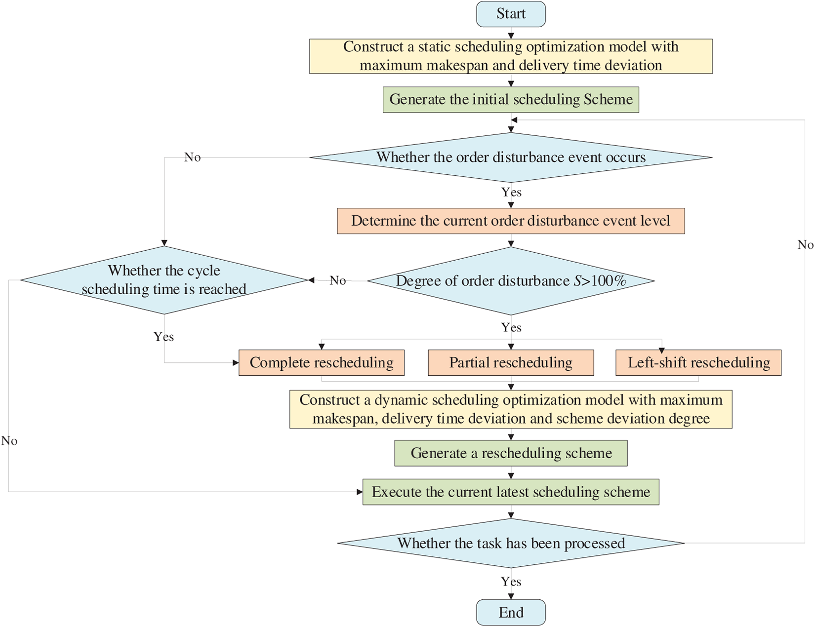
Figure 1: Dynamic scheduling flowchart based on the degree of order disturbance

Step 1: Establish a static scheduling model aiming to minimize both the maximum makespan and the delivery time deviation. Generate and implement the initial scheduling plan using the proposed IMOGWO.

Step 2: Determine whether order disturbance has occurred. If so, proceed to the next step; otherwise, proceed to Step 4.

Step 3: Evaluate the level of the current order disturbance event and calculate the order disturbance degree S. If S>100\% , proceed to Step 5; otherwise, proceed to the next step.

Step 4: Determine whether the scheduled cycle time has been reached. If so, execute the complete rescheduling strategy; otherwise, proceed to Step 7.

Step 5: Select an appropriate dynamic scheduling mode according to Section 3.2 of this paper

Step 6: Establish a dynamic scheduling optimization model considering the maximum makespan, delivery time deviation, and scheme deviation degree. Generate and update the rescheduling plan using the proposed IMOGWO.

Step 7: Execute the current latest scheduling scheme.

Step 8: Determine whether all tasks have been processed. If so, terminate the procedure; otherwise, return to Step 2.

4  Algorithm Design

4.1 Gwo Algorithm

The Grey Wolf Optimizer (GWO) is a swarm intelligence optimization algorithm, simulating the collaborative hunting behavior of grey wolf packs [17]. In solving the optimization problem, the optimal three individuals in the current population are denoted as α, β, and δ, called the leader wolves, and the other individual wolves (denoted as ω) continuously adjust their positions under the guidance of the positioning of the three leader wolves, and approach towards the optimal direction in the search space. Due to space constraints, the specific implementation process of the GWO algorithm is detailed in Reference [17].

4.2 Imogwo Algorithm

The Multi-Objective Grey Wolf Optimizer (MOGWO), proposed by Mirjalili et al. in 2016, extends the single-objective GWO by introducing an external archive to store current non-dominated optimal solutions and modifying the leader selection strategy [23]. However, when solving complex optimization problems, MOGWO still suffers from problems such as easy to falling into a local optimal solution and poor population diversity. Therefore, this paper makes the following improvements to the MOGWO algorithm in Reference [23].

4.2.1 Encoding and Decoding Strategies

The GWO algorithm was originally proposed to solve continuous problems, but the HFSP is a discrete problem. To better integrate the GWO algorithm with HFSP, in terms of process and machine arrangement, they should be divided into two corresponding parts. These two parts form a chromosome, serving as a feasible encoding scheme for HFSP. Therefore, this paper designs a “job-machine” two-layer encoding strategy.

The first layer is the job code: the first digit represents the job number, the second digit represents the job’s processing batch, and the occurrence frequency of the job number indicates the number of its operations.

The second layer is the machine code: each machine code denotes the index of the alternative processing machine set corresponding to the job in the first layer.

Each two-layer code corresponds to a scheduling scheme, specifying the processing machine selected for each operation of each job. The size and number of job subbatches are determined before applying the algorithm, so only the job batch needs to be reflected in the code. Take 3 jobs with 3 operations as an example, where the 3rd job is divided into 2 batches and the others are 1 batch each, as illustrated in Fig. 2a. The job code is [31, 21, 21, 32, 11, 31, 32, 11, 21, 31, 11, 32], and the machine code is [1, 2, 1, 3, 1, 2, 1, 2, 1, 2, 1, 2]. The represented operation sequence is {O31,1, O21,1, O22,1, O31,2, O11,1, O32,1, O32,2, O12,1, O23,1, O33,1, O13,1, O33,2}, where O32,1 denotes the 2nd operation of the 1st batch of job 3. The processing machine numbers corresponding to each operation are sequentially {M1, M2, M4, M3, M1, M5, M4, M5, M6, M7, M6, M7}.

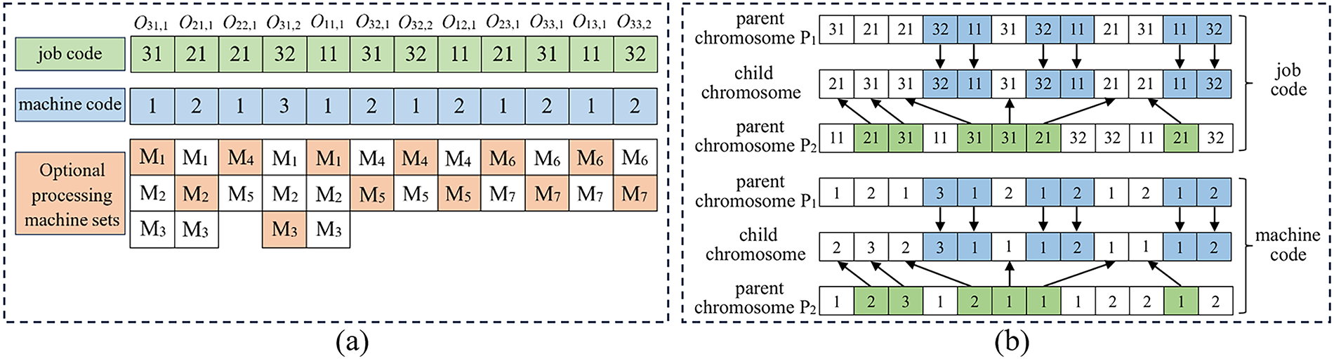
Figure 2: Two-layer encoding and decoding (a) and POX crossover example (b)

During decoding, the designed time-driven two-stage decoding strategy is adopted. Following the logic of “determining the basic order first and then optimizing local efficiency”, the genes of the operation sequence are traversed from left to right to determine the processing sequence of all operations.

In the first stage, the job processing sequence and machine assignment are determined based on the encoding. By encoding to define the process and machine, the common infeasible solution of “reverse process sequence” is avoided, ensuring that the solution complies with the hard timing constraints of HFSP. At the same time, it prevents the increase in computational complexity caused by the coupling of “machine selection” and “timing sequence” in the subsequent stages, reducing interference for the local optimization in the second stage.

In the second stage, the principle of “shortest processing completion time in the current stage” is followed for sorting. The specific process involves screening candidate operations, calculating the expected completion time, and determining the sorting within the stage. All operations of workpieces that have completed the previous stage processing and have not entered the current stage are taken as candidate operations. For each candidate operation, the expected completion time on the current machine is calculated by combining the current idle time of its dedicated machine (i.e., the completion time of the previous operation on the machine) and the processing time of the operation itself (expected completion time = machine idle time + operation processing time). They are then arranged in ascending order of expected completion time, and the operation that can make the machine complete its work faster is prioritized for initiation.

From the perspective of the quality improvement mechanism of the HFSP solution, this two-stage strategy first avoids unfeasible solutions through the determination of operations and machines in the first stage to ensure the basic quality of the solution. Second, it reduces in-stage congestion through local optimization in the second stage, shortening the global makespan.

4.2.2 Opposition-Based Learning Initialization Population Strategy

The standard GWO algorithm utilizes a random initialization strategy, which often fails to ensure the diversity of the initial population. To address this issue, this paper introduces an opposition-based learning initialization strategy. The specific steps are as follows:

(1)   Randomly generate n grey wolf individuals denoted as xij within the decision space of the problem to form the initial population P1.

(2)   Construct an opposite population P2 corresponding to P1 using the principle of opposition-based learning. The opposite individual xij′ is defined as: xij′=s−xij+1, where s is the total number of operations of the jobs.

(3)   Merge the initial population P1 and the opposite population P2 to form a combined population with 2n grey wolf individuals. Sort the 2n individuals using non-dominated sorting, rank each layer of Pareto solutions, and select the top n individuals with the best fitness as the final initial population.

4.2.3 Crossover and Mutation Strategies

To enhance the global search capability of the MOGWO algorithm during the iteration process, crossover and mutation operations are incorporated to strengthen the algorithm’s ability to escape local optima.

The crossover operation is the main means of the algorithm to generate new individuals. This study employs POX crossover to perform crossing on both job codes and machine codes, with the specific crossing process illustrated in Fig. 2b. Firstly, the crossover is performed on the job code, two parent chromosomes P1 and P2 are randomly selected, assuming the initial job set W={11,21,31,32}. The job set is divided into two subsets W1={11,32} and W2={21,31}, and the genes containing W1 in P1 are copied to the child chromosomes without changing their positions in the process of copying; and then the genes containing W2 in P2 are moved to the child chromosomes sequentially in accordance with the order. After the job code crossover operation is completed, the machine code is crossover in accordance with the job code crossover method. This is done to ensure that the processing machine assigned to each operation of every job remains as an optional processing machine.

Mutation operations are applied to the job codes and machine codes after POX crossing. A dual-operation dynamic mutation strategy is designed in this paper, encompassing two distinct mutation operations. A random selection of one of these operations is performed during the implementation process.

(1)   Job Code Mutation: Generate two positions randomly within the length of the solution, swap the job codes of the two positions, and synchronously exchange their corresponding machine codes to ensure machine feasibility.

(2)   Machine Code Mutation: Randomly select multiple positions within the solution length, reassign the machine code in the position, and carry out the mutation following the principle of large allocation probability for short processing time.

4.2.4 Variable Neighborhood Search

To further enhance the local search capability of the algorithm, the local optimization ability is strengthened through a customized neighborhood structure; a VNS containing multiple neighborhood structures is designed [24]. Performing a local search on all population individuals would increase computational time and reduce efficiency. Therefore, to balance computation reduction and diversity preservation, only partial individuals (α, β, and δ) in the population are selected for VNS. The following three neighborhood search structures are employed in this paper.

N1: Randomly select an operation from the current solution. If the operation has multiple alternative machines, choose the machine with the minimum processing time from its alternative machine set.

N2: Find the machine with the largest load from the current solution, randomly select an operation to be processed on that machine, and randomly select a machine to replace it from its set of available machines.

N3: Randomly select two different jobs and an operation position, then swap the machine allocations of the two jobs at this position.

In conducting a VNS, the process begins by determining the current solution. Subsequently, the aforementioned operations are executed sequentially. If a more optimal solution is produced using the neighborhood structure N1, it replaces the current solution, and the process continues with the same neighborhood structure. However, if no improvements can be made to the current solution using N1, the search then progresses to the next neighborhood structure. This systematic shift continues until the predetermined termination iteration number has been reached.

4.2.5 Specific Steps of IMOGWO Algorithm

The flowchart of the IMOGWO Algorithm is shown in Fig. 3. The detailed steps are as follows:

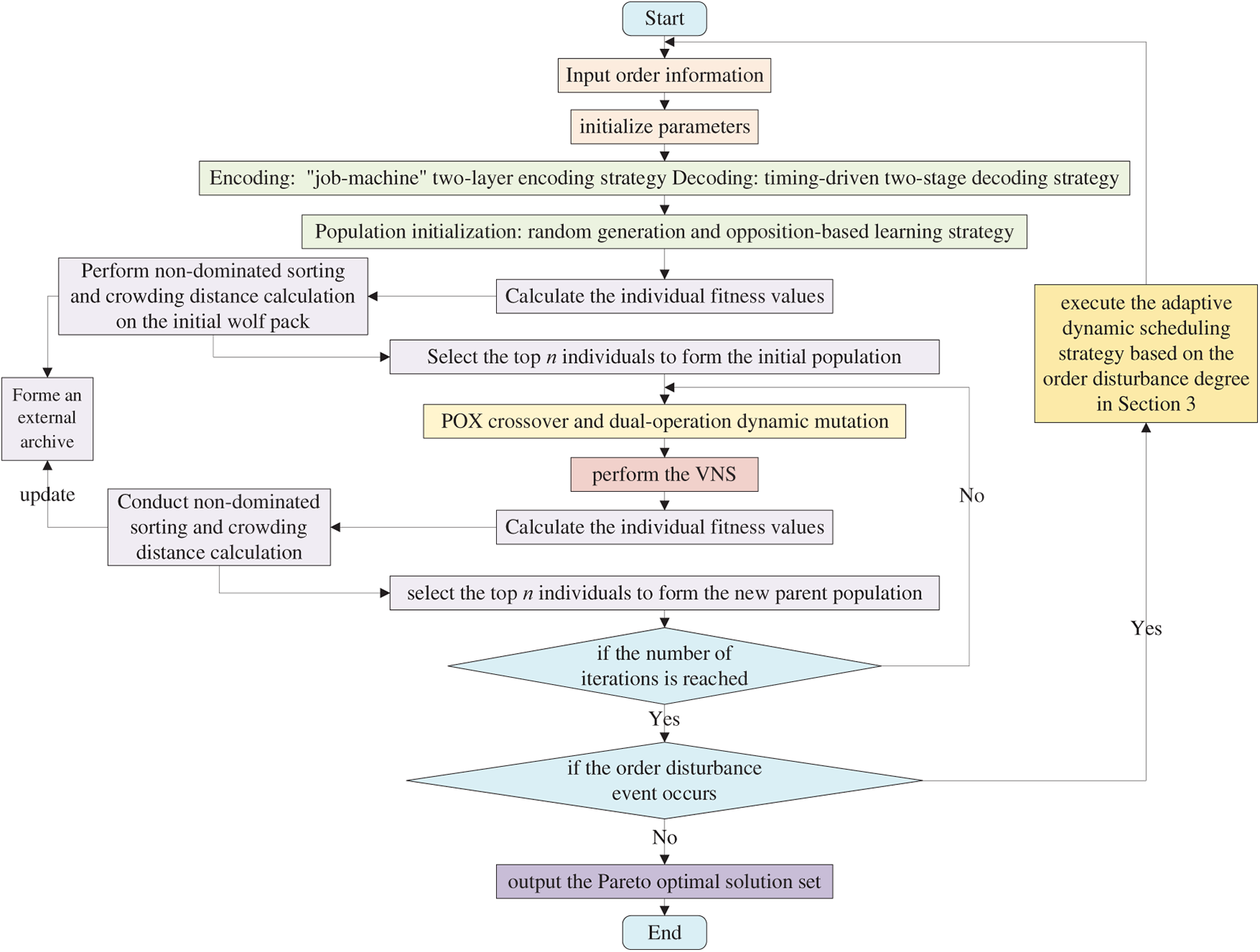
Figure 3: Flowchart of IMOGWO algorithm

Step 1: Input order information and initialize algorithm parameters.

Step 2: Population initialization. Generate the population using a random strategy with the two-layer coding method. Construct an opposite population via opposition-based learning, merge the two populations, decode using the time-driven two-stage decoding strategy, and calculate the individual fitness value.

Step 3: Perform non-dominated sorting and crowding distance calculation on the initial wolf pack. Select the top n individuals to form the initial population, and store the Pareto optimal solutions in an external archive.

Step 4: Randomly select two parent chromosomes and perform POX crossover and dual-operation dynamic mutation.

Step 5: Partial individuals (α, β, and δ) in the population perform the VNS.

Step 6: Calculate the individual fitness values, conduct non-dominated sorting and crowding distance calculation, update the external archive, and select the top n individuals to form the new parent population.

Step 7: Judge if the number of iterations is reached; if so, execute step 8, otherwise, execute steps 4–6.

Step 8: Judge if the order disturbance event occurs; if so, execute the adaptive dynamic scheduling strategy based on the order disturbance degree in Section 3; otherwise, output the Pareto optimal solution set.

5  Experimental Simulation and Case Analysis

5.1 Experiment Design and Parameter Setting

The algorithm proposed in this paper is implemented in MATLAB R2022b, running on a Windows 11 operating system with an Intel(R) Core(TM) i5-12500H processor (2.50 GHz) and 16 GB RAM. To verify the effectiveness of the algorithms in scenarios of different sizes and complexities, 12 sets of test cases are designed. The parameters of the test cases are as follows: the number of jobs n∈{10,20,30,50}, referring to the TAillard test set to cover different scales [25]; the number of operations j∈{3,5,8}, corresponding to the combination of less-to-many-stage processes, which is in line with the logic of stage division in the domain-classical test sets FT10 and Mk04 [26]; the processing data is generated randomly, where the number of parallel machines e is an integer between the interval [2, 3], covering the typical capacity configuration of a hybrid flow processing shop; the processing time of each operation is an integer between the interval [1, 10], and the delivery date as an integer in the interval [5, 15] to simulate order urgency in tight, normal, and loose layers.

5.2 Selection of Evaluation Metrics

In multi-objective optimization, algorithm performance is primarily reflected in the convergence, uniformity, and distribution of the Pareto front solutions. This study employs the Inverted Generational Distance (IGD) and Hypervolume Indicator (HV) as performance evaluation metrics. IGD represents the average distance from each point on the true Pareto front to the nearest point on the obtained Pareto front, calculated by summing and averaging the distances between these points to evaluate the algorithm’s convergence and diversity. Notably, lower IGD values suggest superior comprehensive performance [27]. HV denotes the volume of the objective space bounded by the non-dominated solution set and a dominated reference point (worst point), representing the coverage of non-dominated solutions in the objective space to comprehensively assess convergence and diversity. Here, larger HV values denote improved comprehensive performance [28]. The true Pareto front is constructed by combining all non-dominated solutions from all algorithms and removing dominated solutions from the combined set.

5.3 Validation of the Effectiveness of Improved Strategies

To effectively verify the improvement mechanisms of the IMOGWO algorithm, this paper conducts ablation experiments on the improved components of the algorithm, using IGD and HV values as evaluation metrics. In Tables 3 and 4, IMOGWO and three variant algorithms, along with their corresponding results, are listed. Among them, IMOGWO1, IMOGWO2, and IMOGWO3 correspond to the IMOGWO algorithm modified by removing the opposition-based learning initialization population strategy, the POX crossover and dual-operation dynamic mutation strategy, and the VNS strategy, respectively. In the experiments, the population size of the algorithm is set to 50, the maximum number of iterations is 200, and the capacity of the external archive is 50. Parameter A is linearly decreased from 2 to 0, and parameter C is randomly generated within the interval [0, 2]. The crossover rate and mutation rate for IMOGWO, IMOGWO1, and IMOGWO3 are 0.8 and 0.1, respectively. All other settings follow those in Reference [23]. To avoid the randomness of the algorithm, each test case is run 10 times in a loop, with the optimal values highlighted in bold.

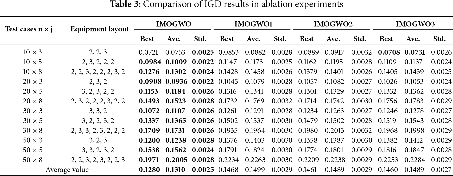
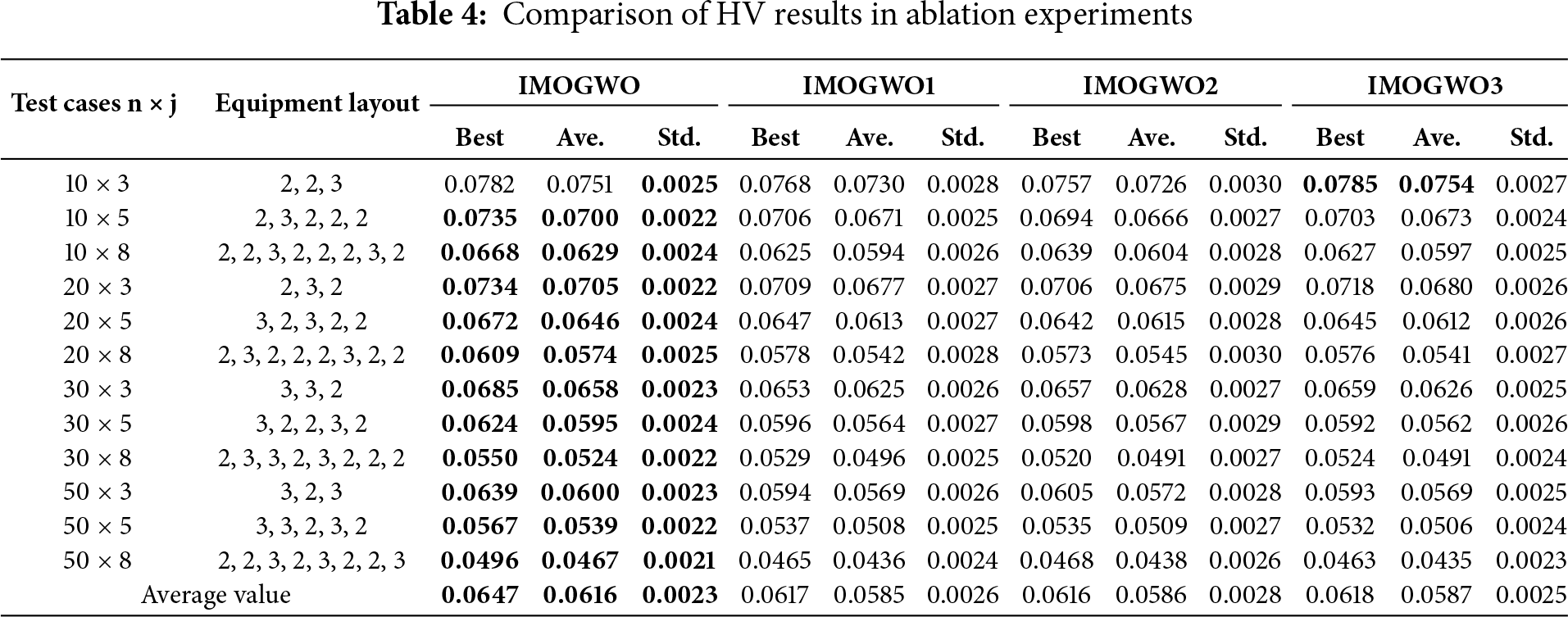
From the comparison results in Tables 3 and 4, it can be observed that the optimal value, average value, and standard deviation of IGD obtained by IMOGWO are 0.1280, 0.1310, and 0.0025, respectively; meanwhile, the optimal value, average value, and standard deviation of HV achieved by IMOGWO are 0.0647, 0.0616, and 0.0023, respectively. All of these metrics are superior to those of the other three algorithms. In the small-scale 10 × 3 test cases, the optimal values and average values of IGD and HV under the IMOGWO3 algorithm are superior to those of IMOGWO, while IMOGWO exhibits better stability. This is because the solution space of this instance is simple, and the global optimum is easily reached by the initial search, while the variable neighborhood search in IMOGWO fails to achieve optimal performance due to redundant computations and the risk of overfitting. On the whole, in most test cases, the optimal values, average values, and standard deviations of IGD and HV for the IMOGWO algorithm are all superior to those of the three variant algorithms with one improved strategy removed. These results verify the effectiveness of each improved strategy.

5.4 Performance Analysis of IMOGWO Algorithm

To analyze the performance of the IMOGWO algorithm in solving the hybrid flow shop multi-objective scheduling optimization model, its operational results are compared with mature and classical MOGWO, MOPSO, and NSGA-II algorithms [23,29,30]. The parameter settings of these algorithms are presented in Table 5. To avoid algorithmic randomness, each test case is run 10 times in cycles, and the maximum, minimum, and average values of the indicators are taken as the final results. Table 6 presents the comparison results of IGD for the four algorithms. Table 7 presents the comparison results of HV for the four algorithms. The optimal value is displayed in bold. Fig. 4 presents the boxplots of IGD and HV for the four algorithms.

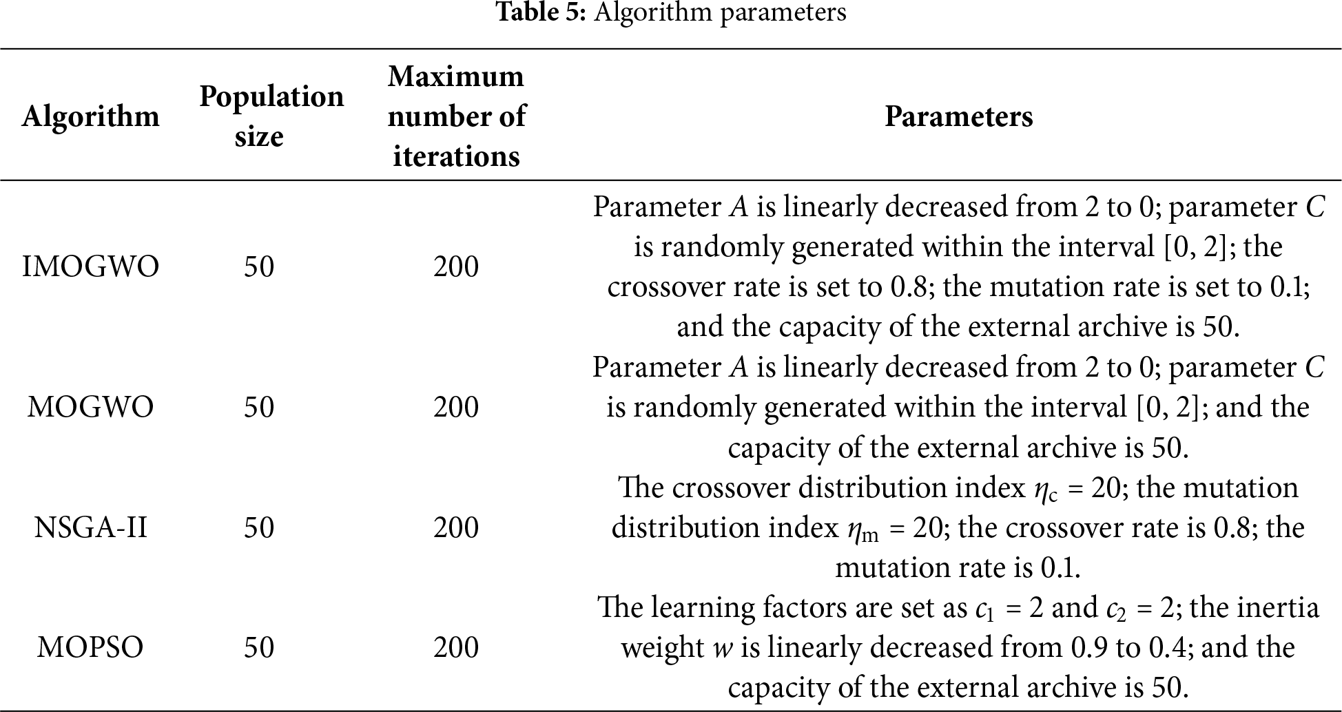
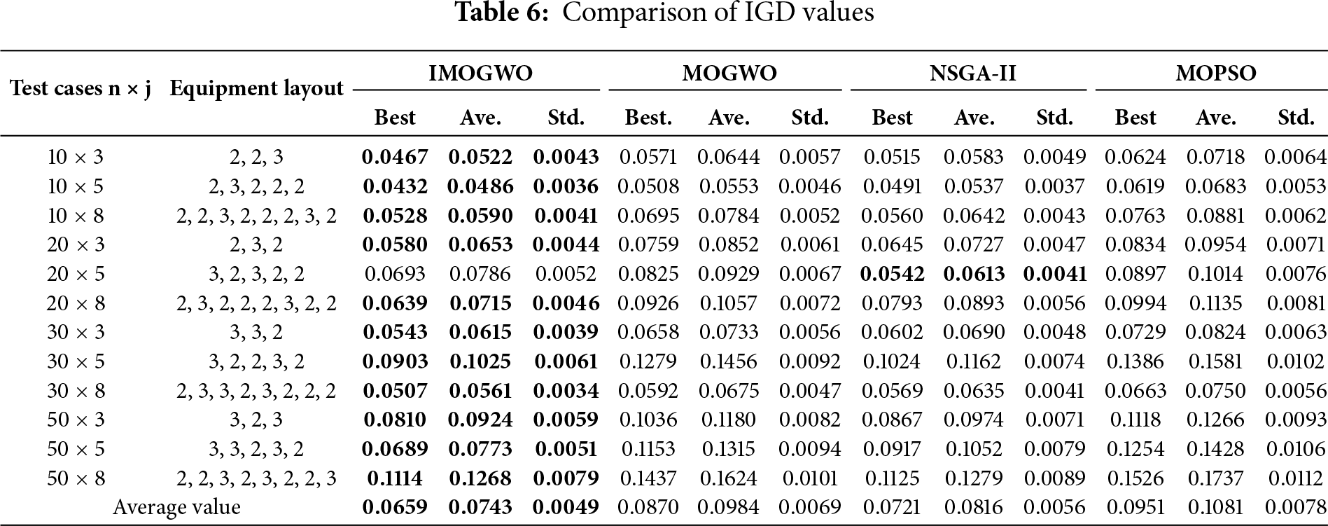
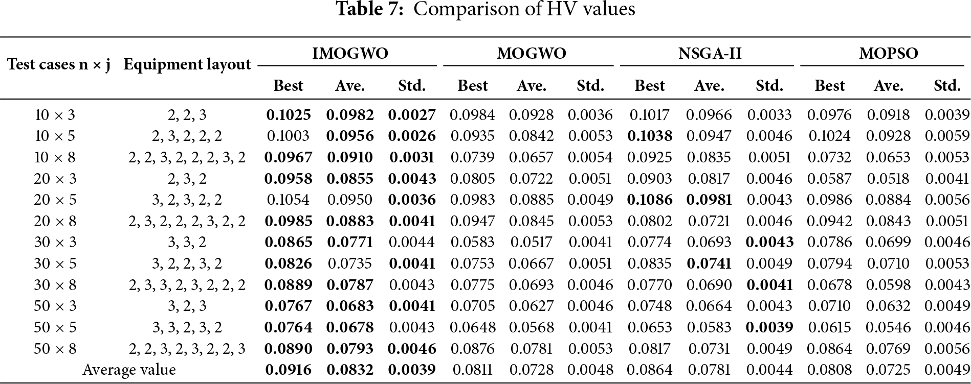
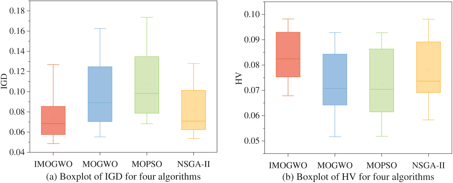
Figure 4: Boxplots of four algorithms

Analysis based on Tables 6 and 7 reveals that the optimal value, average value, and standard deviation of IGD obtained by IMOGWO are 0.0659, 0.0743, and 0.0049, respectively; meanwhile, the optimal value, average value, and standard deviation of HV achieved by IMOGWO are 0.0916, 0.0832, and 0.0039, respectively. All of these metrics are superior to those of the other three algorithms. NSGA-II exhibits a certain degree of competitiveness only in a small number of test cases, and its overall performance is slightly inferior to that of IMOGWO. Meanwhile, MOGWO and MOPSO perform poorly in terms of average IGD and average HV, and they also show insufficient stability. Thus, it can be concluded that the IMOGWO algorithm demonstrates superior comprehensive performance compared to the other three algorithms in solving the HFSP.

As shown in Fig. 4, the boxplots of IMOGWO are flatter than those of the other three algorithms, indicating smaller variance and better stability. The IGD boxplot reveals that IMOGWO has a lower median line than the other three algorithms. Although the difference from NSGA-II is marginal, IMOGWO’s boxplot exhibits significantly greater flatness. The HV boxplot shows that IMOGWO has a notably higher median line than the other three algorithms. These indicate that the non-dominated solution set obtained by IMOGWO is of better quality.

A comparative analysis of the Pareto fronts for the four algorithms is conducted using a random selection of test cases from the 12 instances, as illustrated in Fig. 5. It can be seen that the non-dominated solution set obtained by IMOGWO is located in the lower left of the rest of the algorithms, which is closer to the approximate optimal Pareto front. This indicates that IMOGWO achieves superior accuracy than the comparative algorithms in solving the hybrid flow shop multi-objective scheduling problem.

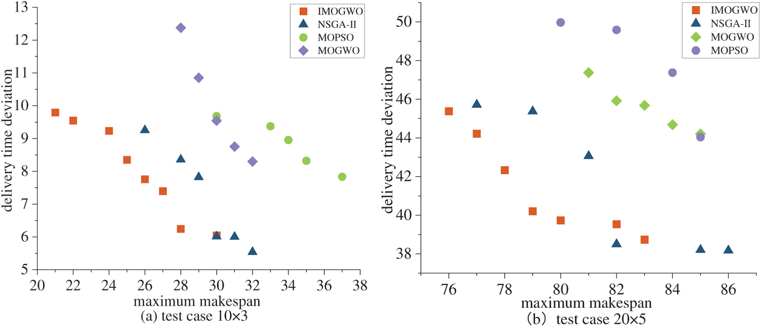
Figure 5: Comparison of Pareto fronts for 4 algorithms

5.5 Case Analysis

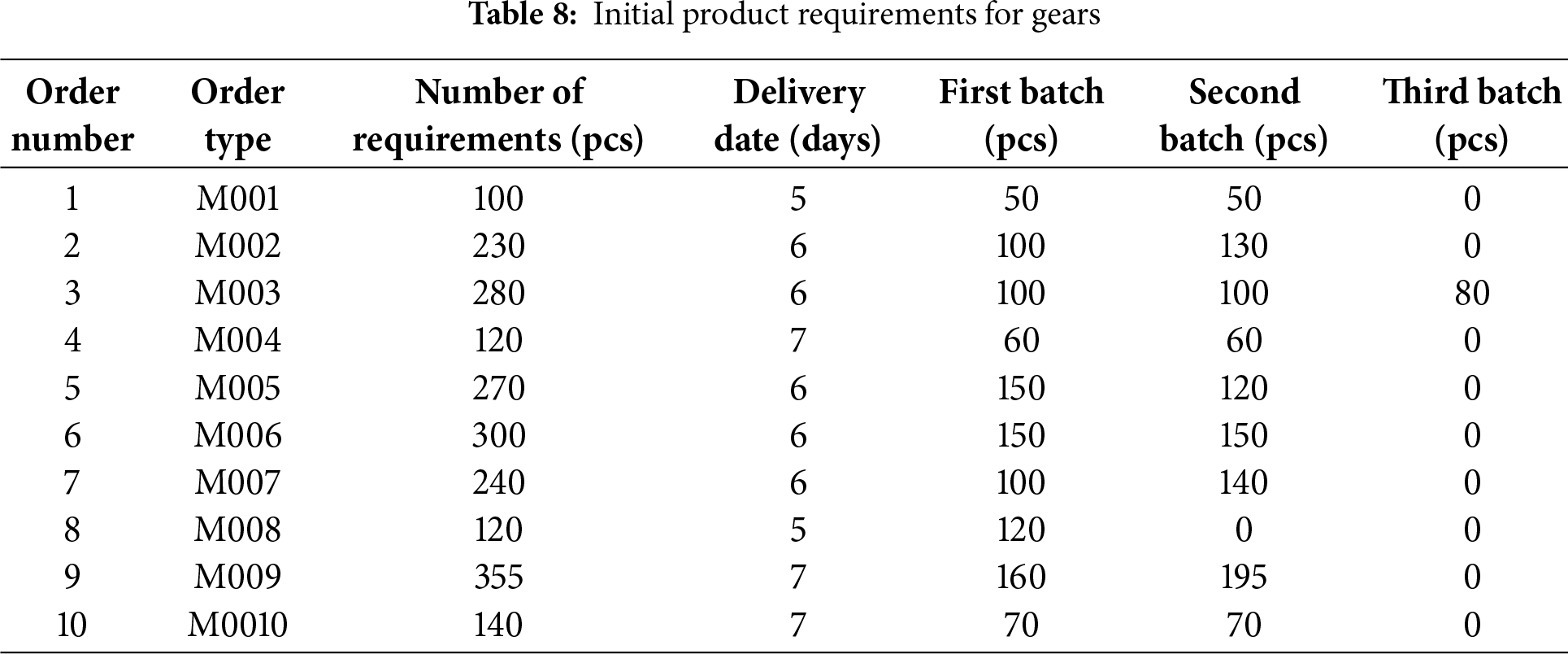
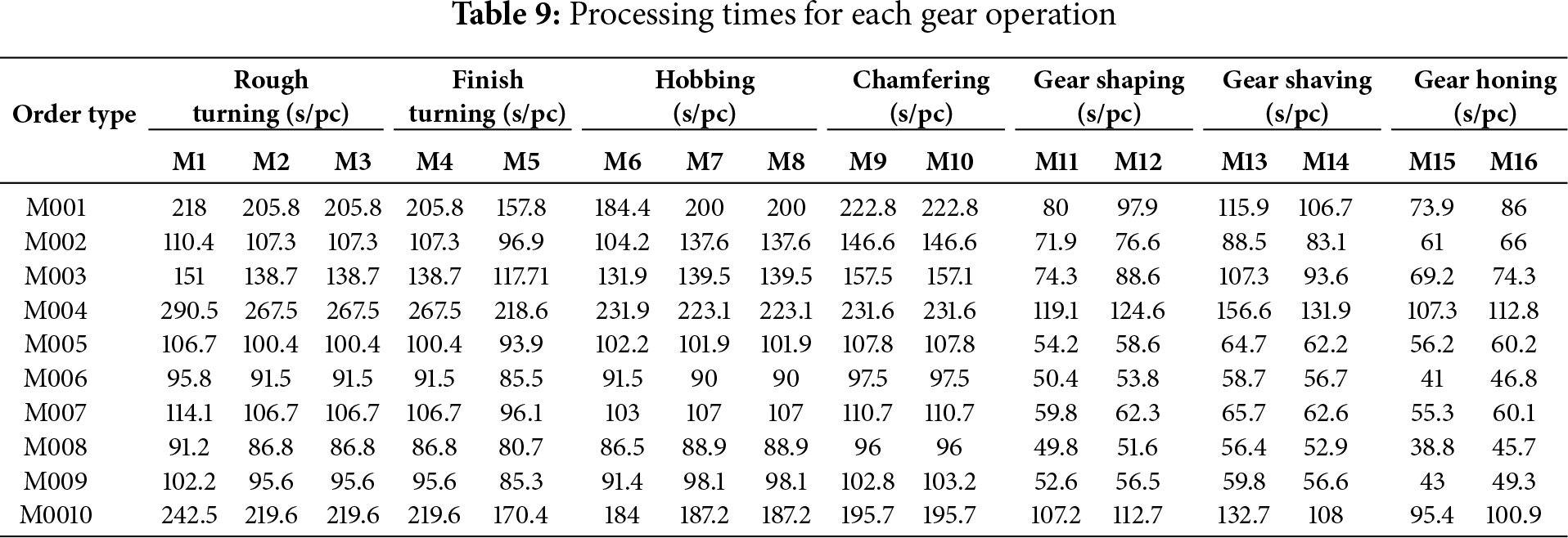
The gear processing shop of a certain enterprise was taken as the research object for analysis. The initial product requirements for gears within a week are shown in Table 8, and the processing times for each gear operation are listed in Table 9. The rated processing time for each machine in the enterprise’s production shop is 8 h per day, and the number of gear production batches and batch sizes are determined based on the shop’s historical experience.

Based on the above information, the static scheduling problem in the first phase was solved. Considering the actual production needs of the enterprise, the initial scheduling Gantt chart is generated by selecting the scheme with the minimum maximum makespan as shown in Fig. 6. The products of different orders are represented by different colors, the batch of the order is represented by the second digit, and the operation is represented by the third digit. For example, 6-2-1 indicates the 1st operation of the 2nd batch of jobs in order 6.

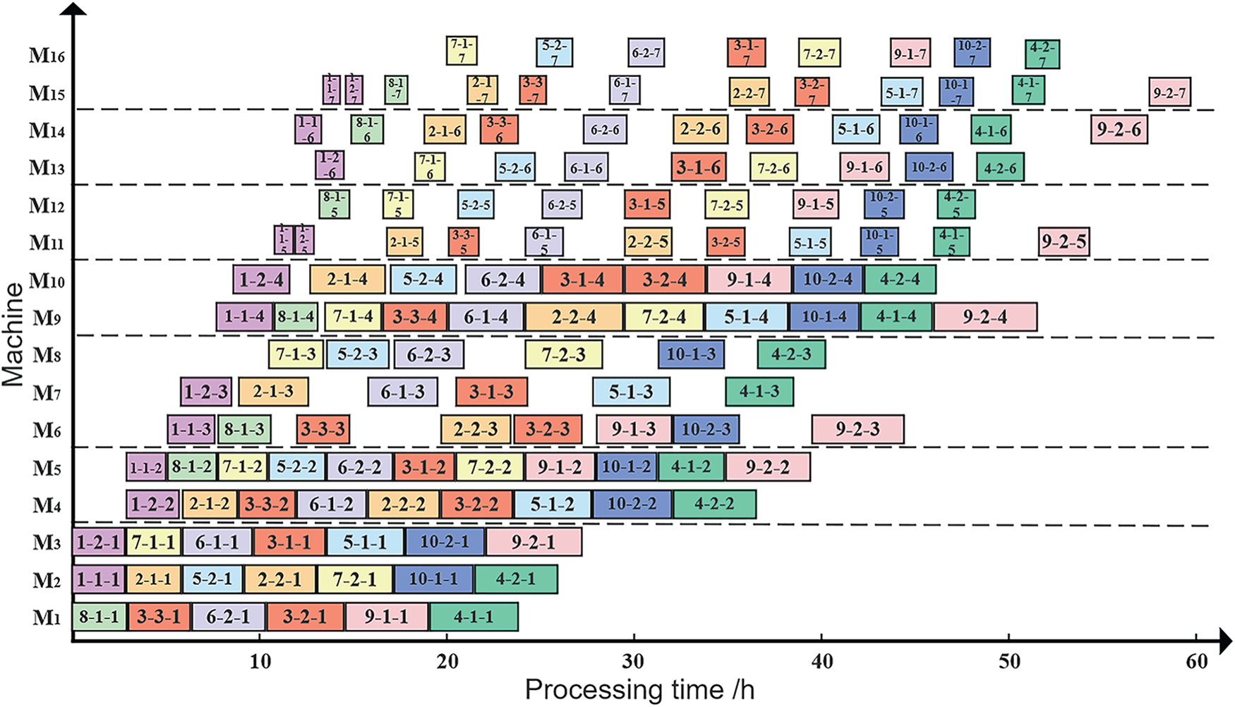
Figure 6: Initial scheduling Gantt chart

After scheduling using the model and algorithm proposed in this paper, all the operations are better scheduled. The maximum makespan is 59.8h, and the delivery time deviation is 12.81 h.

On this basis, the dynamic scheduling under order disturbance in the second phase was verified. Two order disturbance scenarios with different degrees, namely order insertion and order expediting, were designed. Order cancellation is simply eliminated from the scheduling plan, and the remaining unfinished processes are shifted left, which is not shown here due to space constraints.

(1)   Order insertion

At the 23rd hour, new order 11 (product type M008, quantity 80, delivery date 32 h) and order 12 (product type M001, quantity 50, delivery date 32 h) are received. According to Eqs. (16) and (17), the results are β1,β2=1.03125, α1,α2=1.5, ∑k=1h1T¯1,k=11.15, ∑k=1h2T¯2,k=15.183. ∑k=1h1T¯1,k and ∑k=1h2T¯2,k are respectively the sum of the average processing times of new order 11 and order 12 at each operation. The processing time data is derived from Table 8, and the time unit needs to be converted to hours. The order disturbance degree S calculated from Eq. (15) is as follows:

S=1.5×1.03125×11.15+1.5×1.03125×15.18359.8−23×100% =110.7% >100% 

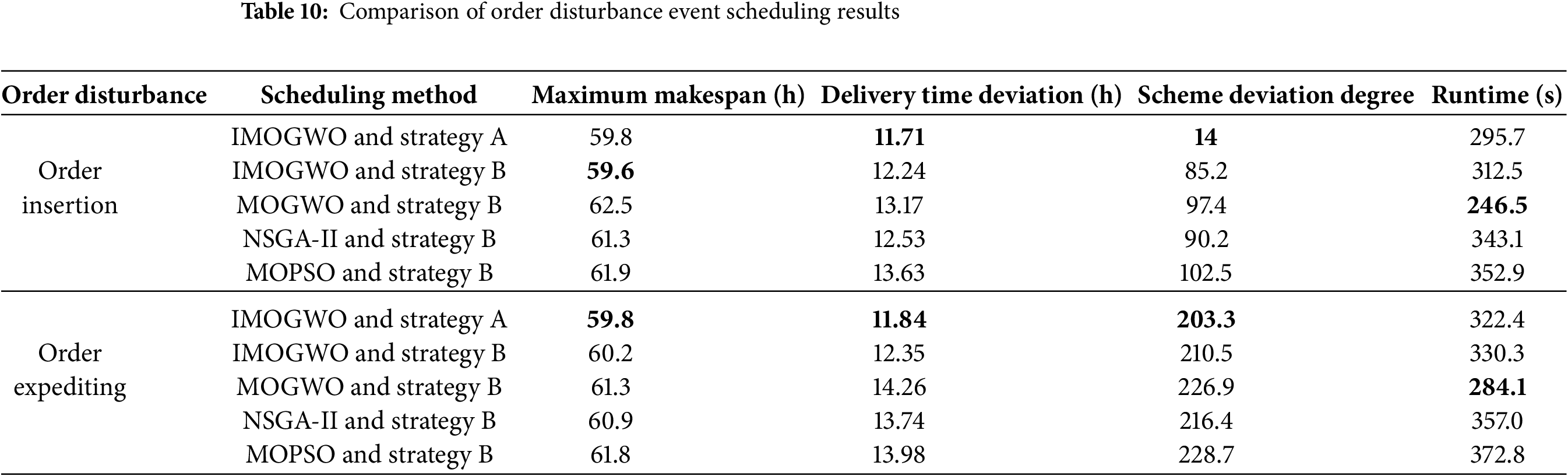
It shows that the order insertion disturbance at this time has a greater impact on the production line, and the original scheduling plan has been difficult to support the current production requirements. Thus, the event-triggered scheduling strategy is invoked to implement dynamic scheduling. To reduce unnecessary scheduling adjustment costs and maintain production stability, partial rescheduling is performed based on the original scheduling plan. The dynamic scheduling Gantt chart for job insertion is shown in Fig. 7a. Inserting new orders during machine idle time effectively addresses the disturbance caused by order insertion. The completion times of Order 11 and Order 12 are 52.9 and 55.3 h, respectively, with delivery times of 29.9 and 32.3 h. Order 11 meets the delivery date of 32 h, whereas Order 12 exceeds the delivery date by only 0.3 h. The maximum makespan of all orders is 59.8 h, identical to that of the initial scheduling scheme. The delivery time deviation is 11.71 h, and the schedule deviation degree is 14.

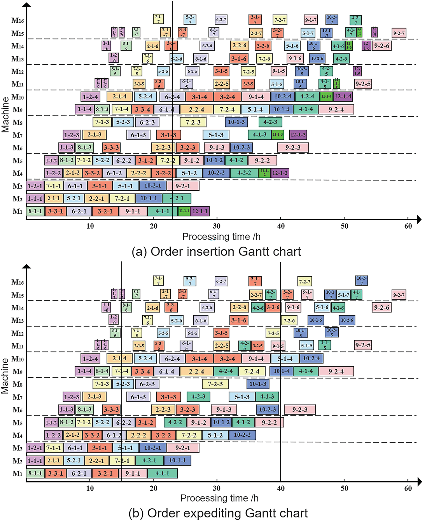
Figure 7: Order disturbance Gantt chart

(2)   Order expediting

At the 15th hour, the delivery date of 60 jobs in order 4 is shortened from 56 to 40 h. In the initial scheduling scheme, the completion time of order 4 is 52.8 h, which exceeds the new delivery date of 40 h. According to Eqs. (16) and (17), the results are β1=1.025, α1=2, ∑k=1h1T¯1,k=22.617. ∑k=1h1T¯1,k represents the sum of the average processing times of expediting order 4 across each operation. The processing time data were derived from Table 6, with the time unit converted to hours. The order disturbance degree S calculated from Eq. (15) is as follows:

S=2×1.025×22.61759.8−15×100% =103.5% >100% 

The order expediting disturbance at this stage indicates a significant impact on the production line. Similarly, the original scheduling plan has been difficult to support the current production requirements, so the event-triggered scheduling strategy is invoked to implement dynamic scheduling. Partial rescheduling is insufficient to meet the current production demands, necessitating complete rescheduling. The dynamic scheduling Gantt chart for the order expediting scenario is shown in Fig. 7b. The delivery time of 60 jobs in order 4 is 39.4 h, satisfying the expediting requirement. The maximum makespan of all orders remains 59.8 h, consistent with the initial scheduling scheme. The delivery time deviation is 11.84 h, and the schedule deviation degree is 203.3.

The scheduling results comparison for order disturbance events is shown in Table 10, with optimal solutions in boldface. The adaptive dynamic scheduling strategy proposed in this study is denoted as strategy A, and the complete rescheduling strategy is referred to as strategy B. Under order insertion disturbance, although the maximum makespan of the IMOGWO algorithm with strategy A is 0.34% higher than that of strategy B, the delivery time deviation and schedule deviation degree are both lower; specifically, the scheme deviation degree is 83.6% lower. When strategy B is adopted, the three objective function values under the IMOGWO algorithm are all smaller than those of the other three algorithms. Under order expediting disturbance, the IMOGWO algorithm combined with strategy A achieves the best values for all three objective functions compared with the other four comparison cases. Under both disturbance scenarios, due to the additional improved strategies incorporated into the IMOGWO algorithm compared to MOGWO, its runtime has slightly increased, but it still falls within the allowable range for actual shop scheduling. Moreover, in comparison with the other two algorithms, NSGA-II and MOPSO, its runtime is shorter.

Case validations demonstrate that the adaptive dynamic scheduling strategy based on order disturbance degree and the IMOGWO algorithm proposed in this paper can effectively address order disturbance events, ensuring both rapid response to order disturbance and stability of the production system.

6  Conclusion and Future Works

This paper addresses the dynamic scheduling problem of hybrid flow shops under order disturbances and establishes a dynamic scheduling model by comprehensively considering three objectives: maximum makespan, delivery time deviation, and scheme deviation degree. To avoid excessive or insufficient scheduling times in actual production, an adaptive dynamic scheduling strategy based on order disturbance degree and an IMOGWO algorithm is proposed for the solution. Specifically, an opposition-based learning strategy is introduced to initialize the population to ensure population diversity; aiming at the problem that the algorithm tends to fall into local optima during solution, the POX Crossover strategy, dual-operation dynamic mutation strategy, and the VNS strategy are incorporated.

Experimental results demonstrate the efficacy and comprehensive performance of the IMOGWO algorithm and model in addressing the multi-objective HFSP. Instance verification for different order disturbance scenarios indicates that the IMOGWO algorithm, combined with the adaptive dynamic scheduling strategy and model, possesses significant advantages in addressing order disturbances.

However, current research exhibits limitations in verifying generalization capabilities. Experiments rely on randomly generated instances and single case studies, focusing solely on order disturbances within an overly idealized environment. Therefore, future research will expand the scale and scope of experimental data to thoroughly validate the effectiveness and comprehensive performance of models and algorithms in larger-scale, actual production with diverse configurations. We will further incorporate other dynamic disturbance events present in actual production, such as machine failures. Additionally, we will explore more complex constraints to better align with practical requirements, including transportation constraints, labor constraints, and others.

Acknowledgement: None.

Funding Statement: This work was funded by National Key Research and Development Program Projects of China under Grant No. 2020YFB1713500.

Author Contributions: The authors confirm contribution to the paper as follows: Conceptualization, Feng Lv and Huili Chu; methodology, Huili Chu; software, Huili Chu; validation, Huili Chu; formal analysis, Huili Chu; investigation, Feng Lv and Huili Chu; data curation, Huili Chu; writing—original draft preparation, Huili Chu; writing—review and editing, Feng Lv and Huili Chu; visualization, Huili Chu; supervision, Feng Lv, Cheng Yang and Jiajie Zhang; project administration, Feng Lv and Huili Chu; funding acquisition, Feng Lv. All authors reviewed the results and approved the final version of the manuscript.

Availability of Data and Materials: The authors confirm that the data supporting the findings of this study are available within the article.

Ethics Approval: Not applicable.

Conflicts of Interest: The authors declare no conflicts of interest to report regarding the present study.

References

1. Ruiz R, Vázquez-Rodríguez JA. The hybrid flow shop scheduling problem. Eur J Oper Res. 2010;205(1):1–18. doi:10.1016/j.ejor.2009.09.024. [Google Scholar] [CrossRef]

2. Duan J, Wang J. Robust scheduling for flexible machining job shop subject to machine breakdowns and new job arrivals considering system reusability and task recurrence. Expert Syst Appl. 2022;203(1):117489. doi:10.1016/j.eswa.2022.117489. [Google Scholar] [CrossRef]

3. Branke J, Mattfeld DC. Anticipation and flexibility in dynamic scheduling. Int J Prod Res. 2005;43(15):3103–29. doi:10.1080/00207540500077140. [Google Scholar] [CrossRef]

4. Yang Y-Y, Qian B, Hu R, Li Z, Zhang Z-Q, Jin H-P, et al. Deep reinforcement learning algorithm incorporating problem characteristics for dynamic multi-objective permutation flow-shop scheduling problem. Swarm Evol Comput. 2025;96(3):101973. doi:10.1016/j.swevo.2025.101973. [Google Scholar] [CrossRef]

5. Li X, Guo A, Yin X, Tang H, Wu R, Zhao Q, et al. A Q-learning improved differential evolution algorithm for human-centric dynamic distributed flexible job shop scheduling problem. J Manuf Syst. 2025;80(4):794–823. doi:10.1016/j.jmsy.2025.04.001. [Google Scholar] [CrossRef]

6. Shi Z, Si J, Zhang J, Pang Z, Chen H, Ding G. A deep reinforcement learning method based on Hindsight experience replay for multi-objective dynamic job-shop scheduling problem. Expert Syst Appl. 2025;284(2–3):127989. doi:10.1016/j.eswa.2025.127989. [Google Scholar] [CrossRef]

7. Liu F, Li X, Lu C, Gong W. Adaptive knowledge-based multi-objective evolutionary algorithm for hybrid flow shop scheduling problems with multiple parallel batch processing stages. Swarm Evol Comput. 2025;95(1):101929. doi:10.1016/j.swevo.2025.101929. [Google Scholar] [CrossRef]

8. Wang Z, Liao W, Zhang Y. Rescheduling optimisation of sustainable multi-objective fuzzy flexible job shop under uncertain environment. Int J Prod Res. 2024;62(24):8904–20. doi:10.1080/00207543.2024.2354830. [Google Scholar] [CrossRef]

9. Chen R, Wu B, Wang H, Tong H, Yan F. A Q-Learning based NSGA-II for dynamic flexible job shop scheduling with limited transportation resources. Swarm Evol Comput. 2024;90(3):101658. doi:10.1016/j.swevo.2024.101658. [Google Scholar] [CrossRef]

10. Zhu N, Gong G, Lu D, Huang D, Peng N, Qi H. An effective reformative memetic algorithm for distributed flexible job-shop scheduling problem with order cancellation. Expert Syst Appl. 2024;237(3):121205. doi:10.1016/j.eswa.2023.121205. [Google Scholar] [CrossRef]

11. Wei L, He J, Guo Z, Hu Z. A multi-objective migrating birds optimization algorithm based on game theory for dynamic flexible job shop scheduling problem. Expert Syst Appl. 2023;227(1):120268. doi:10.1016/j.eswa.2023.120268. [Google Scholar] [CrossRef]

12. Angel-Bello F, Vallikavungal J, Alvarez A. Fast and efficient algorithms to handle the dynamism in a single machine scheduling problem with sequence-dependent setup times. Comput Ind Eng. 2021;152(3):106984. doi:10.1016/j.cie.2020.106984. [Google Scholar] [CrossRef]

13. Zou Y, Lu C, Yin L, Wen X. Multi-level subpopulation-based particle swarm optimization algorithm for hybrid flow shop scheduling problem with limited buffers. Comput Mater Contin. 2025;84(2):2305–30. doi:10.32604/CMC.2025.065972. [Google Scholar] [CrossRef]

14. Wang Z-C, Pan Q-K, Gao L, Miao Z-H, Sang H-Y. A variable-representation discrete artificial bee colony algorithm for a constrained hybrid flow shop. Expert Syst Appl. 2024;254(3):124349. doi:10.1016/j.eswa.2024.124349. [Google Scholar] [CrossRef]

15. Zeng L, Shi J, Li Y, Wang S, Li W. A strengthened dominance relation NSGA-III algorithm based on differential evolution to solve job shop scheduling problem. Comput Mater Contin. 2024;78(1):375–92. doi:10.32604/CMC.2023.045803. [Google Scholar] [CrossRef]

16. Liu Y, As’arry A, Hassan MK, Hairuddin AA, Mohamad H. Review of the grey wolf optimization algorithm: variants and applications. Neural Comput Appl. 2024;36(6):2713–35. doi:10.1007/s00521-023-09202-8. [Google Scholar] [CrossRef]

17. Li X, Xie J, Ma Q, Gao L, Li P. Improved gray wolf optimizer for distributed flexible job shop scheduling problem. Sci China Technol Sci. 2022;65(9):2105–15. doi:10.1007/s11431-022-2096-6. [Google Scholar] [CrossRef]

18. Lin C, Cao Z, Zhou M. Learning-based grey wolf optimizer for stochastic flexible job shop scheduling. IEEE Trans Autom Sci Eng. 2022;19(4):3659–71. doi:10.1109/TASE.2021.3129439. [Google Scholar] [CrossRef]

19. Zheng J, Chen S. A Q-learning multi-objective grey wolf optimizer for the distributed hybrid flowshop scheduling problem. Eng Optim. 2025;57(9):2609–28. doi:10.1080/0305215X.2024.2410844. [Google Scholar] [CrossRef]

20. Tosun Ö, Marichelvam MK, Tosun N. A literature review on hybrid flow shop scheduling. Int J Prod Res. 2020;12(2):156–94. doi:10.1504/IJAOM.2020.108263. [Google Scholar] [PubMed] [CrossRef]

21. Zhou L, Zhang L, Fang Y. Comparison of production-triggering strategies for manufacturing enterprises under random orders. Engineering. 2021;7(6):798–806. doi:10.1016/j.eng.2021.03.012. [Google Scholar] [CrossRef]

22. Cui H, Li X, Gao L, Xiang Z, Zhou W, Yu Y et al. Cooperation-based bi-level rescheduling method for multi-objective distributed hybrid flow shop with unrelated parallel machines under multi-type disturbances. Int J Comput Integr Manuf. 2025:1–23. doi:10.1080/0951192X.2025.2478005. [Google Scholar] [CrossRef]

23. Mirjalili S, Saremi S, Mirjalili SM, Coelho LdS. Multi-objective grey wolf optimizer: a novel algorithm for multi-criterion optimization. Expert Syst Appl. 2016;47(6):106–19. doi:10.1016/j.eswa.2015.10.039. [Google Scholar] [CrossRef]

24. Alkhateeb F, Abed-alguni BH, Al-rousan MH. Discrete hybrid cuckoo search and simulated annealing algorithm for solving the job shop scheduling problem. J Supercomput. 2022;78(4):4799–826. doi:10.1007/s11227-021-04050-6. [Google Scholar] [CrossRef]

25. Taillard E. Benchmarks for basic scheduling problems. Eur J Oper Res. 1993;64(2):278–85. doi:10.1016/0377-2217(93)90182-M. [Google Scholar] [CrossRef]

26. Jiang T, Zhang C. Application of grey wolf optimization for solving combinatorial problems: job shop and flexible job shop scheduling cases. IEEE Access. 2018;6:26231–40. doi:10.1109/ACCESS.2018.2833552. [Google Scholar] [CrossRef]

27. Fu Y, Gao K, Wang L, Huang M, Liang Y-C, Dong H. Scheduling stochastic distributed flexible job shops using an multi-objective evolutionary algorithm with simulation evaluation. Int J Prod Res. 2025;63(1):86–103. doi:10.1080/00207543.2024.2356628. [Google Scholar] [CrossRef]

28. Zheng J, Zhao J, Zhao S. A heuristic method for multi-objective hybrid flow shop scheduling problem with parent-child relationships and space constraints. Int J Prod Res. 2025;63(7):2431–55. doi:10.1080/00207543.2024.2403126. [Google Scholar] [CrossRef]

29. Shao X, Liu W, Liu Q, Zhang C. Hybrid discrete particle swarm optimization for multi-objective flexible job-shop scheduling problem. Int J Adv Manuf Technol. 2013;67(9):2885–901. doi:10.1007/s00170-012-4701-3. [Google Scholar] [CrossRef]

30. Yu W, Zhang L, Ge N. An adaptive multiobjective evolutionary algorithm for dynamic multiobjective flexible scheduling problem. Int J Intell Syst. 2022;37(12):12335–66. doi:10.1002/INT.23090. [Google Scholar] [CrossRef]