A TimeXer-Based Numerical Forecast Correction Model Optimized by an Exogenous-Variable Attention Mechanism

1  Introduction

Numerical forecast correction technology analyzes and processes local features by integrating observational data with the numerical forecast results generated by model forecast products, thereby achieving more accurate forecast results. Traditional correction methods such as MOS (Model Output Statistics) [1] cannot efficiently handle the increasingly massive data, exhibit limited capability in processing dense grid areas, and consume substantial computational resources [2]. Due to the powerful data processing capability of artificial intelligence technology, more and more intelligent correction products have emerged, which address the shortcomings of traditional correction methods [3].

1.1 Intelligent Correction Methods Based on Machine Learning

In 2024, Yang et al. [4] proposed a short-term load forecasting algorithm based on a multi-scale deep neural network. This algorithm decomposes sequences into high and low frequency components and combines autoregression, bidirectional GRU (Gated Recurrent Unit), and an attention mechanism to model temporal features. It outperforms traditional methods in prediction accuracy but suffers from higher computational complexity and limited training efficiency. In 2025, Guo et al. [5] constructed a numerical weather prediction correction model using convolutional neural networks. Evaluation Indexes including R² and RMSE demonstrate that this model can significantly reduce errors, but its accuracy decreases in marine wind speed correction due to the influence of air-sea interactions. Liu et al. [6] developed the TabNet-MTL model on the basis of multi-task deep learning. By integrating short-term and long-term statistical features and thermodynamic factors to correct both wind speed and direction, this model significantly improves the forecasting accuracy of near-surface wind fields, but it is limited to validation with station data and hard to extend to grid point forecasting. Alharthi et al. [7] built a wind power prediction framework integrating NSGA (Non-dominated Sorting Genetic Algorithm)-III and DRNN-LSTM (Deep Recurrent Neural Network-Long Short-Term Memory), which combines feature selection with deep recurrent networks to enhance model generalization. Nonetheless, it incurs high training costs and fails to consider the impact of external environments, restricting its adaptability and stability in complex scenarios.

1.2 Intelligent Correction Methods of Marine Elements Based on Deep Learning

In 2024, Lawal et al. [8] proposed a multivariate multi-step prediction model based on a BiLSTM (Bidirectional Long Short-Term Memory) network. This model significantly improves prediction accuracy in deep-water areas by capturing bidirectional temporal dependencies, but is limited to single-station training and exhibits insufficient generalization ability. Xiao and Lu [9] presented a hybrid model combining Conformer and LSTM. This model outperforms traditional models on NOAA (National Oceanic and Atmospheric Administration) multi-station datasets at the expense of higher computational cost. Gregory et al. [10] conducted sea ice bias correction based on convolutional neural networks combined with data augmentation, which enhances the prediction accuracy of sea ice concentration, while the cross-variable applicability of this method remains to be verified. In 2025, Da Silva et al. [11] applied LSTM to correct errors in significant wave height prediction; compared with linear regression, this approach significantly reduces prediction errors and demonstrates strong temporal modeling capability and stability.

To fully explore the potential feature relationships between historical marine data and initial forecast data and enhance the accuracy of numerical forecast correction for marine environmental variables, this paper constructs an intelligent correction model based on the TimeXer framework by introducing an exogenous-variable attention mechanism. In addition to capturing temporal correlations, the model explicitly considers spatial dependencies among multiple oceanic variables across temporal-spatial feature scales inspired by the successful application of spatial attention in marine-related tasks [12]. This design enables the model to effectively exploit historical observations, initial forecasts, and multi-scale spatial data, thereby improving the precision of forecast correction.

The main contributions of this paper are as follows.

(1) Aiming at the problem of lower data processing efficiency in traditional machine learning models, this paper constructs a DNN (Deep Neural Network) to process historical data and initial forecast data. Compared with traditional machine learning models, DNN has better data representation capabilities, can learn complex function mappings, and perform well on large-scale datasets.

(2) To address the issues of limited research on the correction of marine elements and insufficient mining of feature correlations among relevant variables, the paper proposes a numerical forecast correction model for sea surface temperature in marine environments. The model is built upon the TimeXer framework with an exogenous-variable attention mechanism. The mechanism enhances the model’s capability to extract both explicit and implicit correlations between historical temporal-spatial data and initial forecast data, thereby improving correction efficiency and reducing prediction errors.

(3) Compared with the TimeXer and PatchTST models, the proposed model achieves the best performance on the core evaluation metric, namely MSE (Mean Squared Error), significantly outperforming the comparative models. The experiment results validate the advancement and effectiveness of the proposed method in multivariate time series forecasting tasks.

2  Materials and Methods

2.1 Experiment Data

The experiment data were selected from the Global Ocean Physics Analysis and Forecast product provided by the GLO MFC (Global Monitoring and Forecasting Centre) of the CMEMS (Copernicus Marine Environment Monitoring Service) in accordance with the requirements of the National Key R&D Program Project. Specifically, a subset of data was extracted from the GLO MFC’s daily-updated Global Ocean Physics Analysis and Forecast product. This product integrates satellite and in-situ observations to provide state-of-the-art reanalysis data, which largely reflects the real development and variation trends of marine variables. The data are widely used to observe, understand, and predict the state of the marine environment [13]. Thus, this paper selected historical reanalysis data that more accurately represent the real marine environment as the experiment data to enhance the effectiveness of feature extraction and obtain more accurate forecast values of oceanic variables.

In the process of model training and verification, sea surface temperature reanalysis data covering the sea area from 109°20′00″ E to 110°5′00″ E and latitude from 11°25′00″ N to 12°10′00″ N were used for a total of 6 months from July 2023 to December 2023. The data set is a NetCDF (Network Common Data Form) grid data file. Due to the large amount of NetCDF grid file data and the data format is not convenient for machine learning model processing, this paper preprocesses the NetCDF grid reanalysis data of sea surface temperature before data input model training. Read NetCDF grid data files to find sea surface temperature data within the scope of experimental research, build experimental research data sets, and convert data formats into data file formats more suitable for machine learning models.

2.2 A Numerical Forecast Correction Model of TimeXer Enhanced by an Exogenous-Variable Attention Mechanism

2.2.1 The TimeXer Model

Deep models exhibit remarkable performance in time series forecasting. However, due to the characteristics of partial observations in practical applications, focusing solely on target variables (i.e., endogenous variables) is generally insufficient to ensure accurate predictions.

In 2024, Wang et al. [14] proposed the TimeXer model, a novel Transformer architecture designed for time series forecasting that integrates exogenous variable information to enhance the prediction accuracy of endogenous variables. In practical applications, time series are often influenced by various external factors, and relying solely on historical data of endogenous variables cannot effectively capture these complex relationships. Therefore, TimeXer incorporates exogenous variables to enrich the information available for forecasting. This approach is particularly relevant in fields such as meteorology and power systems, where external conditions exert significant impacts on the target sequences.

In contrast to existing multivariate or univariate forecasting paradigms that either treat all variables equally or ignore exogenous information, TimeXer focuses on time series forecasting incorporating exogenous variables. By introducing exogenous variables, it enables more comprehensive understanding of the correlations and causal relationships among variables, thereby enhancing performance and inter-pretability. Through a well-designed embedding layer, TimeXer equips the classical Transformer with the ability to coordinate endogenous and exogenous information, while utilizing self-attention and variable cross-attention to capture dependencies in the temporal and variable dimensions, respectively. TimeXer also features good scalability, with its structure being easy to extend and modify. However, TimeXer primarily focuses on temporal dependencies and neglects spatial correlations. For temporal-spatial data such as ocean forecasting, spatial correlations are equally crucial, and TimeXer cannot explicitly model these spatial relationships in an efficient manner.

To address this issue, the paper optimizes the TimeXer model by introducing an exogenous variable attention mechanism. The mechanism better captures the interrelationships among exogenous variables, enables feature mining of these variables, captures their temporal and spatial dependencies, and further guides the endogenous variable forecasting task to improve prediction accuracy.

2.2.2 Exogenous Variable Data

The external variable data used in the correction process include historical time dimension data, historical spatial dimension data, original seven-day forecast value obtained from the forecast product, longitude, latitude data and ocean depth data of the target correction point. The specific data amount and data description are as follows.

(1) Historical time dimension data. The time dimension data is extracted based on three timescales in the feature selection process of this paper. According to the prior knowledge of meteorology, in the process of natural climate development, the evolution trend of meteorological elements is highly correlated with the time process, which is manifested in the characteristics of seasonal or cyclical meteorological development trend and the similarity of meteorological elements in the near period. Therefore, this paper selects three time-scale data adjacent to the target prediction time for feature mining, and the expression formula of time-dimension data is shown in Eq. (1).

XTime={XT|T=1,2,3}(1)

where, XTime is the time dimension feature obtained after feature selection operation, XT represents specific feature data of different timescales.

(2) Historical spatial dimension data. In this paper, eight spatial scale data around the target prediction location are selected for feature extraction. Similarly, according to prior knowledge in meteorology, geography and other fields, meteorological element data is highly correlated with the meteorological evolution trend of the surrounding geographical range in space. For example, the climate temperature data in the tropical region is generally higher than that in the polar region, while the climate data in the nearby region does not produce such a gap. Therefore, in order to fully consider the impact of meteorological elements in the adjacent space on the target forecast region, a total of eight adjacent spatial scales were selected for feature mining. The spatial dimension data is shown in Eq. (2).

XSpace={XS|S=1,2,⋯,8}(2)

where, XSpace is the spatial dimension feature obtained after feature selection operation, XS indicates specific feature data of different spatial scales.

(3) Original seven-day forecast data. The original forecast values are also used as exogenous variables to guide the correction task. The original forecast value is derived from the output of classical numerical model prediction products, which contains physical dynamics information and statistical knowledge, and can capture high-dimensional information that can guide the numerical correction task of ocean element prediction. At the same time, physical constraints are introduced to the correction model based on artificial intelligence technology, and the overall efficiency of the model is improved by combining the advantages of deep learning model nonlinear modeling. The original seven-day forecast data are shown in Eq. (3).

XForecast={XF|F=1,2,…,7}(3)

where, XForecast is the original seven-day forecast value data, XF represents the original forecast data under specific different forecast timeliness.

On the whole, the comprehensive representation of exogenous variable data adopted in this paper is shown in Eq. (4).

X={XTime,XSpace,XForecast,XLon,XLat,Xdep}(4)

where, X is the external variable data as a whole, XLon,XLat,Xdep are respectively longitude data, latitude data and ocean depth data of the target correction location.

2.2.3 A Correction Model of Sea Surface Temperature Numerical Prediction by Introduction of External Variable Attention Mechanism

Based on TimeXer model’s embedding strategy for internal and external variables and its advantages in attention mechanism processing, this paper introduces the attention mechanism of external variables to construct a correction model for sea surface temperature numerical prediction. The proposed network structure is shown in Fig. 1.

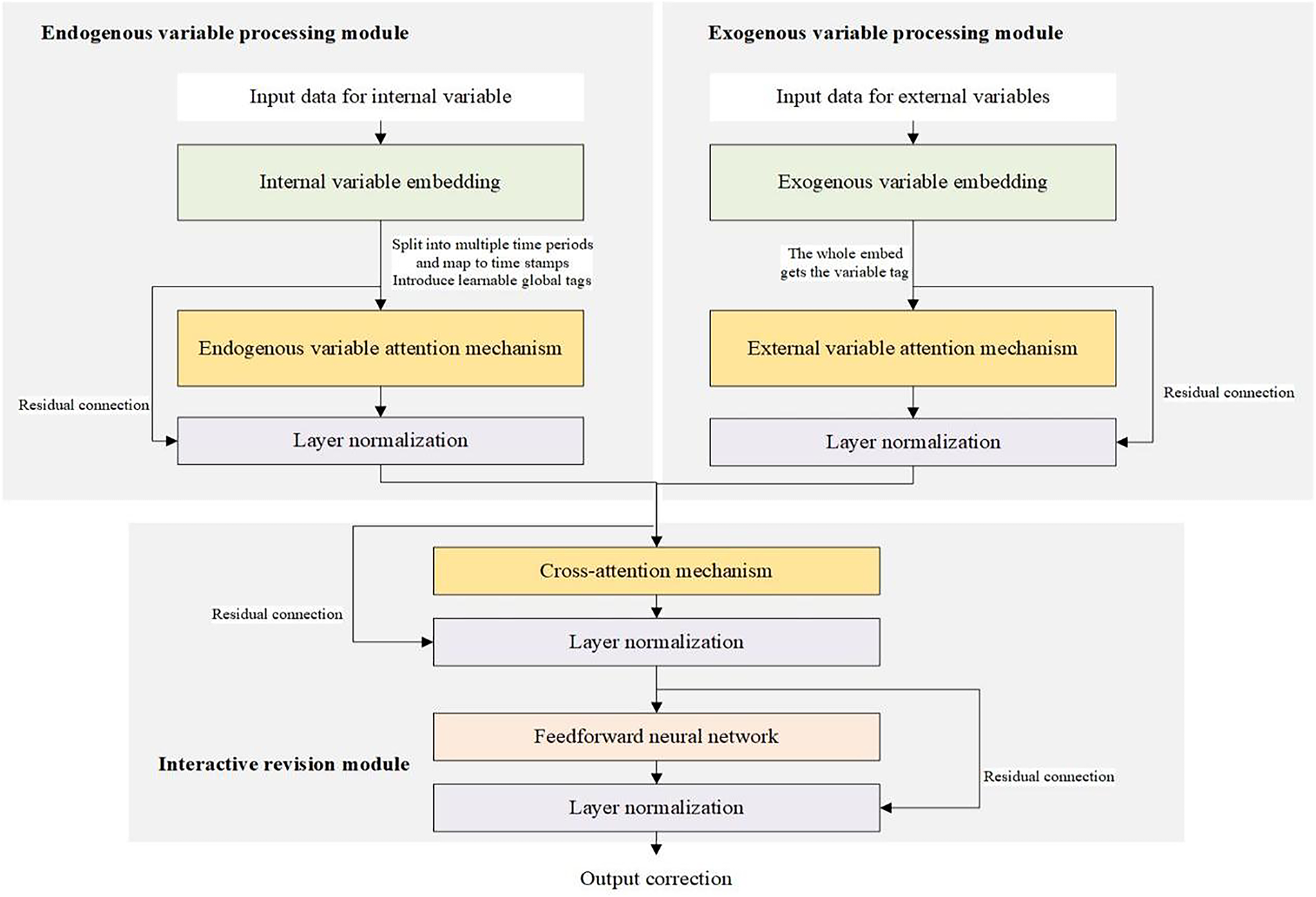
Figure 1: The proposed network structure

The proposed model includes exogenous variable processing module, endogenous variable processing module and interactive revision module. The exogenous variable processing module embeds multiple exogenous variables as a whole to obtain a variable token. Since exogenous variables can provide auxiliary information and potential features to realize the model’s prediction and revision of endogenous variables. Therefore, this paper introduces the exogenous variable attention mechanism on the basis of TimeXer model for feature mining of correlation between multiple exogenous variables.

The endogenous variable processing module splits the endogenous time series variable into multiple time patches, each mapped to a temporal token, and employs self-attention to capture its temporal dependence. At the same time, a learnable global token is introduced as a macroscopic representation of the endogenous variable. The interactive revision module interacts the feature mining results of the endogenous and exogenous variables, and integrates the information of the exogenous variables into the prediction of the endogenous variables through the cross-attention mechanism to realize the revision of the numerical prediction results of the endogenous variables at future time steps. The overall processing flow of the model and related formulas are specifically described as follows.

First, the model receives input data of several exogenous variables and an internal variable, and carries out feature mining processing through the exogenous variable processing module and the internal variable processing module, respectively.

The processing module of exogenous variables embedded the data of exogenous variables in the input model as a whole, took the whole sequence as a variable marker, and mined the overall correlation between exogenous variables. The embedding mapping formula of exogenous variables was shown in Eq. (5).

Vex,i=VariateEmbed(z(i)),i=1,2,3,…,C(5)

where, C is the number of exogenous variables, i indicates the exogenous variable of the i-th term, z(i) denotes the sequence of exogenous variables of the i-th term, and Vex represents the mapped exogenous variable label.

Since exogenous variables play an important role in the prediction correction of endogenous variables, the potential correlation mining between exogenous variables can make a positive contribution to the improvement of the accuracy of endogenous variables. Based on the advantages of self-attention mechanism to extract multivariate correlation, this paper introduces exogenous variable attention mechanism to mine features among multiple exogenous variables, and adopts residual linkage and layer normalization to process exogenous variable features. The overall processing of external variable is shown in Eq. (6).

v~exl=LayerNorm(vexl+Self−Attention(vexl))(6)

where, Vexl is the exogenous variable marker, and l represents the l-th correction module, l=0,⋯,L−1 and Vex0=Vex.

The internal variable processing module first divides the internal variable data of the input model into multiple non-overlapping time periods, and synchronously maps them to the corresponding time period variable markers, so as to reduce the data volume and improve the data processing efficiency. In addition, in the process of data embedding, a learnable global variable tag is also introduced synchronously, which is used as a macro representation of the internal variable and interacts with the external variable in the processing of the subsequent module. The internal variable embedding processing formula is respectively shown in Eqs. (7)–(9).

{S1,S2,S3,…,SN}=Patchify(x)(7)

Pen=PatchEmbed(S1,S2,S3,⋯,SN)(8)

Gen=Learnable(x)(9)

where, x is the sequence of internal variables of the input model, N indicates the number of segmented time periods, Si represents the i-th time period, Pen is the mapped time period variable marker, and Gen denotes the global variable marker that can be learned.

The variable tag data obtained after the two embeddings are combined to obtain the final internal variable tag. The tags of internal variables after data embedding are input into the self-attention module to capture the time dependence between internal variables. The overall processing formula of the internal variable module is shown in Eq. (10).

P^enl,G^enl=LayerNorm([Penl,Genl]+Self−Attention([Penl,Genl]))(10)

where, [Penl,Genl] is the internal variable marker after concatenation, and l indicates the l-th correction module. l=0,⋯,L−1 and Pen0=Pen,Gen0=Gen.

The interactive correction module implements the final intelligent correction output. The exogenous multivariate correlation features and endogenous global variable features extracted by the exogenous variable processing module and the endogenous variable processing module are interacted through the cross-attention mechanism to realize the correlation mining between endogenous variables and exogenous variables. The calculation formula is shown in Eq. (11).

G^enl=LayerNorm(G^enl+Cross−Attention(G^enl,V^exl))(11)

Then, it is mapped through the feed-forward neural network layer. The layer processing formula of feed-forward neural network is shown in Eqs. (12) and (13).

Penl+1=Feed−Forward(P^enl),l=1,2,⋯,L(12)

Genl+1=Feed−Forward(G^enl),l=1,2,⋯,L(13)

Finally, the model correction results are obtained through the linear mapping layer. The square loss function is used to measure the difference between the model correction result and the true value, and guide the model to learn closer to the true value of the internal variable, and finally improve the model correction accuracy. The loss function formula is shown in Eq. (14).

Loss=∑i=1s‖xi−x^i‖22(14)

where, x^=Projection([PenL,GenL]) is the corrected result value obtained after the output result of the internal variable passes through the linear mapping layer.

2.3 An Intelligent Correction Method for Marine Environmental Variables Based on TimeXer with an Exogenous-Variable Attention Mechanism

The specific steps for the proposed method are given below.

(1)   Data preprocessing. Read in the large-scale sea surface temperature NetCDF lattice point reanalysis data file and screen the sea surface temperature data in the target range, construct the overall data set and save it as a table file that is easy to read for the machine learning model. Divide the training dataset, validation dataset and test dataset for subsequent model training and evaluation.

(2)   Model loss function selection. The training of the model involves minimizing the error between the predicted and true values of the model. In this paper, MSE is used as the loss function to realize the error calculation, and gradually guide the model to learn the data. MSE is the average of the squares of the prediction error, and since the distribution of the sea surface temperature data in the ocean reanalysis data is relatively uniform, basically there are no outliers and extreme values, and there is no need to consider the effect of the outliers on the calculation of the error.

Using MSE as the loss function can make the predicted values closer to the expectation of the true values, thus enabling the model to provide more accurate prediction results. On the other hand, since MSE is microscopic, it facilitates model training using optimization algorithms such as gradient descent. Based on the targeted advantages of the mean square error metrics for the prediction problem and dataset, this paper adopts MSE as the loss function during the model training process, and optimizes the model parameters to enhance the accuracy of the prediction outputs by minimizing the loss function. MSE is defined in Eq. (15).

MSE=1n∑i=1n(yi−y^i)2(15)

where, n is the number of samples, yi denotes the true value, and y^i signifies the predicted value.

(3)   Determining model hyperparameters. This paper conducted comparative experiments across multiple hyperparameter combinations to establish the final parameter settings. The model employs the Adam optimizer with an initial learning rate of 0.0001. The maximum number of training epochs is set to be 20, incorporating an early stopping strategy, training is terminated prematurely when no significant improvement is observed on the validation set for five consecutive epochs to prevent overfitting. The batch size was set to 1, and the seed was fixed at 2025 to ensure reproducibility of experimental results. All experiments were conducted on a single GPU environment equipped with a GeForce RTX 3080 (10 GB VRAM). This configuration balances computational efficiency and hardware resource constraints while ensuring stable model convergence.

(4)   Model training. The proposed model is trained using the training dataset, fully exploiting the high-dimensional features or potential features among the exogenous variables and interacting with the global markers of the endogenous variables to obtain the feature representation vector used to guide the model to output the revised results. The degree of difference between the predicted and real values of the model is used to guide the model to update the weights, and the validation dataset is used to test the current training effect of the model in each round of training, and the model training results are saved when the loss value of the model is less than the lowest loss value in the history, and the model training is ended when the training reaches 20 rounds or meets the requirements of the early stopping strategy, and the training result of the model with the lowest loss value is taken as the optimal model for the subsequent The model training result with the lowest loss value is taken as the optimal model for subsequent testing and evaluation.

(5)   Model testing. In order to verify the effectiveness and feasibility of the presented model, a test data set is used to evaluate the forecasting ability of the optimal model. The performance of the model is fully analyzed by calculating the results of the evaluation indexes with the model prediction values and the actual real values.

3  Results and Discussion

To validate the effectiveness of the presented model, experimental comparisons were conducted between the original TimeXer model, the PatchTST model [15], and the model presented herein. Using MSE, MAE, RMSE, MAPE, and MSPE as evaluation metrics, the paper further analyzed the consumption of time resources. The correction performance of each model was assessed for both one-day and seven-day corrections across different historical scales to evaluate correction efficiency. It should be noted that beyond deep learning approaches, recent studies have also explored numerical forecast correction using physically constrained models (e.g., numerical models based on ocean dynamic equations) or physics-deep learning hybrid models [16]. While these methods offer advantages in terms of mechanism interpretability, they often exhibit high sensitivity to initial conditions, boundary conditions, and parameter settings, and incur significant computational costs for predicting high-dimensional ocean variables. In contrast, the proposed model can automatically learn complex correlations among external variables within an end-to-end framework. It captures temporal-spatial dependencies without explicit physical constraint assumptions, achieving higher prediction accuracy while maintaining low computational cost.

3.1 Evaluation Indexes

The evaluation metrics such as MSE, MAE (Mean Absolute Error), RMSE (Root Mean Square Error), MAPE (Mean Absolute Percentage Error), and MSPE (Mean Square Percentage Error) are used in the experiment. MSE and RMSE assess the degree of deviation between the model predictions and the observed values. MAE calculates the mean absolute difference between predicted and observed values, providing a clearer measure of predictive accuracy. MAPE is widely used in practical applications to quantify relative forecasting errors. MSPE evaluates model performance by computing the squared percentage error between predictions and observations, and it is commonly applied in time series forecasting and regression tasks. Collectively, these five metrics enable a comprehensive and effective assessment of the proposed model performance.

By squaring the errors, MSE amplifies the penalty for large deviations, which is particularly crucial in ocean forecasting, where a single substantial prediction error can have far more severe consequences than multiple minor errors. MSE effectively quantifies the robustness of model and its ability to control the impact of outliers.

MSE is the loss function used in the model training process, and the formula is shown in Eq. (15). However, due to the square calculation, the numerical unit is the square of the target variable unit, so the interpretation of the prediction results is different, and RMSE is the square root of MSE, the formula is shown in Eq. (16).

RMSE=MSE=1n∑i=1n(yi−y^i)2(16)

RMSE has the same unit as the original data, so it is more intuitive in explaining the model performance and can directly reflect the size of prediction error, which makes up for the shortcomings of MSE.

Since both MSE and RMSE are sensitive to outliers, large errors will have a greater impact on the evaluation results. Therefore, this paper evaluates the difference degree of model prediction together with MAE to obtain a more comprehensive evaluation of model prediction performance. MAE is a classical evaluation index for accuracy evaluation. The MAE is calculated in Eq. (17).

MAE=1n∑i=1n|yi−y^i|(17)

where, |⋅| represents the absolute value calculation. Since the MAE calculation process does not involve squaring operations, it is less sensitive to outliers and solves the problem of MSE and RMSE outlier sensitivity.

MAPE provides a percentage representation of the prediction error and is dimensionless. The formula is shown in Eq. (18).

MAPE=100%n∑i=1n|yi−y^iyi|(18)

MAPE is often used in prediction tasks, especially when the true value has very little probability of being zero. The revision task is essentially to predict the numerical results, so the MSPE index is used to evaluate the accuracy of the prediction model to evaluate the revised results. The formula for calculating the MSPE is shown in Eq. (19).

MSPE=1n∑i=1n(y^i−yiyi)2(19)

In this paper, model training time, model testing time and total time are used as assessment indicators to compare and analyze the time performance of the presented model. The results of the above eight assessment indicators are synthesized to provide a comprehensive assessment of the performance of the presented model.

3.2 Comparison and Analysis of Experiment Results

The proposed model was analyzed by comparing the prediction results of the three models with the actual values, alongside a comparative analysis using eight objective evaluation metrics. The comparison between the prediction results of the three models and the actual values is shown in Fig. 2.

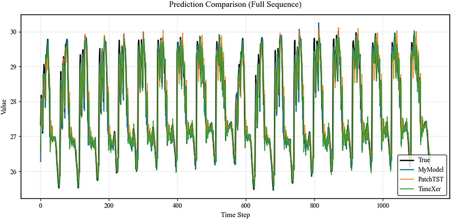
Figure 2: Comparison of observed and predicted values for the three models

In Fig. 2, the TimeXer model exhibits relatively superior control over overall errors, with lower global mean squared error, suggesting an advantage in capturing long-term trends. The PatchTST model shows noticeable lag in certain fluctuation intervals, whereas the proposed model maintains a high level of consistency with the observed sequence across the entire range. Its predicted curve is smoother and better aligned with the true values, indicating improved stability in overall forecasting. To further analyze differences among the models in detailed predictions, the first 200 time steps are selected as a representative interval for magnified comparison, as shown in Fig. 3.

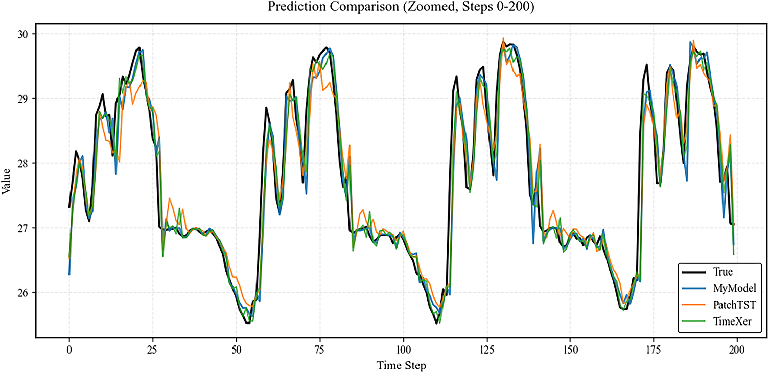
Figure 3: Local magnified interval (the first 200 time steps)

As shown in Fig. 3, the proposed model closely tracks the observed values even in intervals with frequent fluctuations, particularly outperforming the TimeXer and PatchTST models in fitting segments with rapid short-term changes. In contrast, the PatchTST model exhibits lagging deviations at several local peak points, while the TimeXer model, although showing lower overall errors, demonstrates certain limitations in capturing the fine details of rapid fluctuations. Overall, the proposed model demonstrates strong performance in both global prediction accuracy and stability, with particularly notable advantages in detailed representation and robustness.

To further investigate the impact of parameter selection on the experimental results within the proposed network architecture, we set the input historical sequence length to 9 and the output correction horizon to 1 day as the baseline for parameter tuning experiments. A comparative study of activation functions was then conducted to evaluate model performance. The results are presented in Table 1, and the comparison of the four primary metrics is shown in Fig. 4.

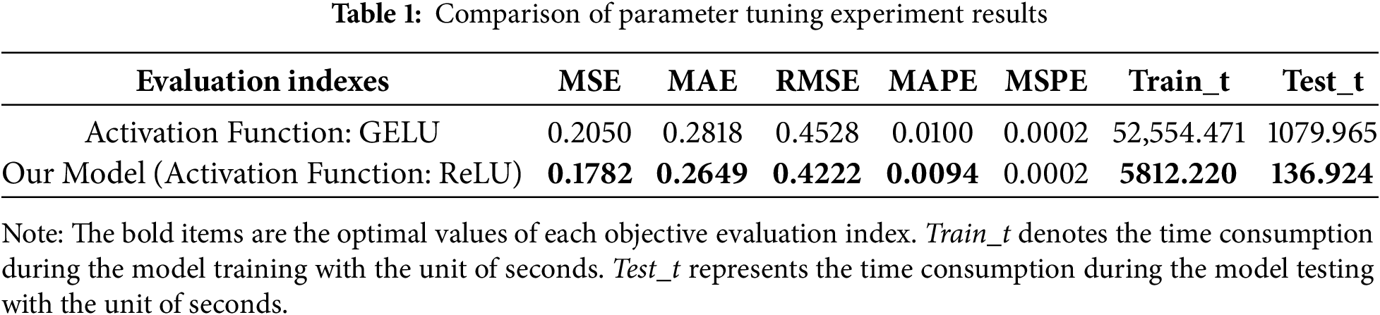
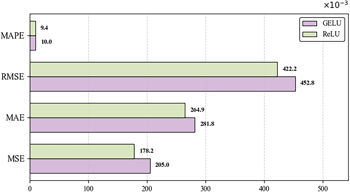
Figure 4: Comparison of parameter tuning results with an input historical sequence length of 9 and an output correction horizon of 1 day

Based on the results of the comparative evaluation, the proposed model with ReLU (Rectified Linear Unit) as the activation function outperforms the model using GELU (Gaussian Error Linear Unit) in several key evaluation metrics. In terms of error analysis, MSPE shows comparable results, while the other four metrics demonstrate decreases, indicating that selecting ReLU enables more accurate forecast corrections. The training and testing times of the proposed model are significantly lower than those of the GELU-based model, reflecting higher computational efficiency. The ReLU activation function is computationally simpler and allows more efficient gradient computation, effectively mitigating the vanishing gradient problem and accelerating model convergence. Consequently, the model with ReLU exhibits much shorter training and testing times compared to the GELU variant.

Overall, the proposed model with ReLU activation demonstrates superior performance in both predictive accuracy and operational efficiency relative to the GELU-based model, exhibiting strong overall performance. ReLU proves to be highly suitable for the proposed framework, effectively enhancing model performance.

To validate the specific impact of the exogenous variable attention mechanism and cross-attention mechanism on model performance, this paper conducted comparative experiments under different input historical sequence lengths and output correction time windows. The experiments were performed by removing either the exogenous variable attention module or the cross-attention fusion module from the proposed model while keeping all other structural components consistent. The experiment results are presented in Table 2.

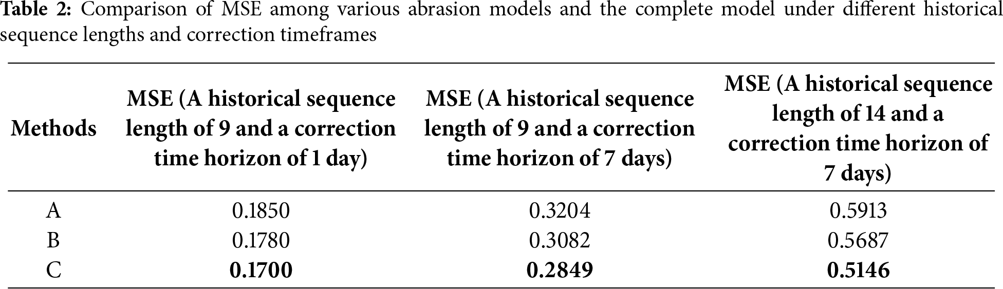
Table 2 demonstrates removing the exogenous variable attention module significantly increases the model prediction error across all correction time horizons. When the input historical sequence length is 9 and the output correction time horizon is 1 day, the MSE increases by approximately 8.8%. and when the input historical sequence length was 14 with a 7-day correction lead time, the increase reached 14.9%. This indicates that the external variable attention mechanism plays a crucial role in extracting multi-temporal-spatial correlation features and suppressing error accumulation. Removing the cross-attention fusion module also led to a decline in model performance, demonstrating that the interactive fusion of internal and external variable features is significant for the overall prediction accuracy of the model. Overall, the complete model achieved the lowest MSE across all correction time horizons, validating the effectiveness and synergistic effect of the designed external variable attention mechanism and cross-attention mechanism in enhancing both short-term and medium-to-long-term correction performance.

The paper also calculated the performance evaluation metrics of the presented model and the two benchmark models through experiments. To more comprehensively assess model performance, we further introduced SSIM (Structural Similarity Index) as a supplementary metric to evaluate the consistency between the model’s predicted field and the observed field in terms of spatial structure and contrast. SSIM ranges from 0 to 1, with values closer to 1 indicating greater spatial structural consistency between predictions and observations. We conducted a combined evaluation considering different historical sequence lengths and correction timeliness. The comparison of evaluation metrics for each model under varying historical lengths and correction timeliness is shown in Table 3. Fig. 5 illustrates the comparison of the core evaluation metric MSE for each model under different historical lengths and correction timeliness.

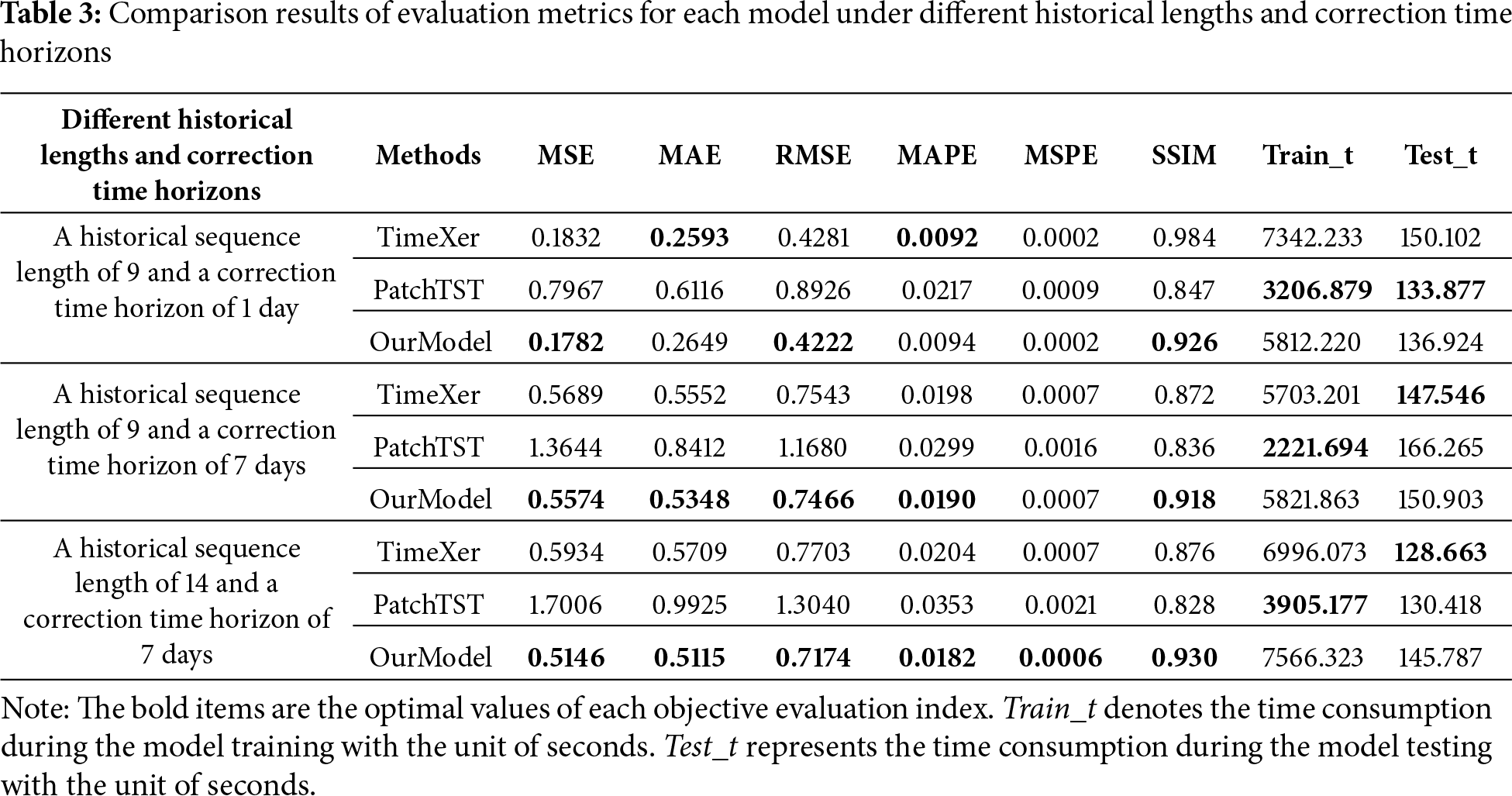
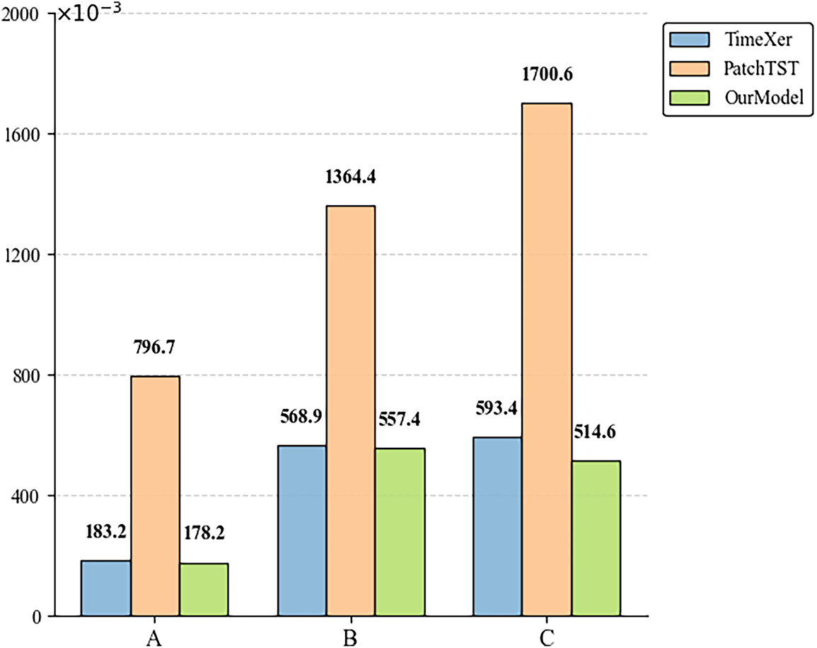
Figure 5: Comparison of the core evaluation metric (namely MSE) for each model under different historical lengths and correction time horizons. A denotes a historical sequence length of 9 and a correction time horizon of 1 day. B denotes a historical sequence length of 9 and a correction time horizon of 7 days. C denotes a historical sequence length of 14 and a correction time horizon of 7 days

As shown in Table 3, when the input historical sequence length is 9 and the output correction timeframe is 1 day, the proposed model attains lower MSE and RMSE than both TimeXer and PatchTST, with only minor increases in MAE (0.056) and MAPE (0.0002) compared with TimeXer. It achieves 2.73% and 1.38% improvements in MSE and RMSE, respectively, while PatchTST shows shorter computation time but noticeably lower accuracy. When the input historical sequence length is 9 and the output correction timeframe is 7 days, the proposed model further improves MSE, MAE, RMSE, and MAPE by 2.02%, 3.67%, 1.02%, and 4.04% over TimeXer, maintaining similar computational cost. when the input historical sequence length is 14 and the output correction timeframe is 7 days, it achieves the best results across all five metrics, improving MSE, MAE, RMSE, MAPE, and MSPE by 13.28%, 10.40%, 6.87%, 10.78%, and 14.29%, respectively, while maintaining comparable time performance to TimeXer.

Overall, Table 3 shows that the proposed model achieves the best comprehensive performance across five error metrics. For short-term (one-day) forecasts, its MSE and RMSE are lower and MSPE comparable to TimeXer. For long-term (seven-day) forecasts, all metrics show clear improvement, reflecting higher accuracy and stability under different horizons. Even with limited historical data, the model maintains robust performance and computational efficiency comparable to TimeXer, while significantly surpassing PatchTST. The SSIM index further confirms its superiority, with average improvements of 5.6% over TimeXer and 9.3% over PatchTST, indicating that the exogenous-variable attention mechanism enhances both prediction precision and spatial structural consistency.

As can be seen from Fig. 5, the proposed model achieves the smallest MSE under different historical lengths and correction time horizons, with overall performance superior to TimeXer and PatchTST. Particularly, when the historical length is 14 and the correction time horizon is 7 days, the MSE of the proposed model drops to 0.5146, which is approximately 13.3% and 69.7% lower than that of TimeXer and PatchTST. The results validate the effectiveness of the exogenous-variable attention mechanism in capturing multi-temporal-spatial feature correlations, thereby significantly boosting the model’s long-term correction accuracy and stability.

4  Conclusions

This paper presents a TimeXer-based numerical forecast correction model optimized by an exogenous-variable attention mechanism. By integrating multi-scale temporal-spatial and initial forecast data as exogenous variables, the model adopts self-attention to capture latent feature associations and improve correction accuracy of endogenous variable correction. Comparative experiments with TimeXer and PatchTST demonstrate its superior short-term and medium-term forecasting accuracy with only a minor increase in computational cost, highlighting its practical value for marine environment forecasting. However, the current study is limited to SST (Sea Surface Temperature) data from July to December 2023 in a specific region of the northern South China Sea, which may affect the model’s generalizability. Future work will expand to multi-region and multi-variable datasets (e.g., salinity, sea level height) and incorporate uncertainty quantification to further enhance the model’s accuracy and interpretability.

Acknowledgement: Not applicable.

Funding Statement: This paper was supported by the National Key Research and Development Program Project (2023YFC3107804), Planning Fund Project of Humanities and Social Sciences Research of the Ministry of Education (24YJA880097), and the Graduate Education Reform Project in North China University of Technology (217051360025XN095-17).

Author Contributions: Yongmei Zhang provided the overall research direction, supervision, and funding support. Tianxin Zhang proposed the framework, method and experiments. Linghua Tian refined the experiment result analysis and revised the manuscript. All authors reviewed the results and approved the final version of the manuscript.

Availability of Data and Materials: Data will be made available on request.

Ethics Approval: Not applicable.

Conflicts of Interest: The authors declare no conflicts of interest to report regarding the present study.

References

1. Glahn HR, Lowry DA. The use of model output statistics (MOS) in objective weather forecasting. J Appl Meteorol. 1972;11:1203–11. doi:10.1175/1520-0450(1972)011<1203:TUOMOS>2.0.CO;2. [Google Scholar] [CrossRef]

2. Yang X, Dai K, Zhu Y. Progress and challenges of deep learning techniques in intelligent grid weather forecasting. Acta Meteorol Sin. 2022;80(5):649–67. [Google Scholar]

3. Dong C, Wang Z, Xie H, Xu G, Han G, Zhou S, et al. Prospect of artificial intelligence in oceanography. J Mar Sci. 2024;42(3):2–27. [Google Scholar]

4. Yang Y, Gao Y, Wang Z, Li X, Zhou H, Wu J. Multiscale-integrated deep learning approaches for short-term load forecasting. Int J Mach Learn Cybern. 2024;15(12):6061–76. doi:10.1007/s13042-024-02302-4. [Google Scholar] [CrossRef]

5. Guo S, Yang Y, Zhang F, Wang J, Cheng Y. Study on bias correction method of ECMWF surface variable forecasts based on deep learning. Renew Energy. 2025;239:122132–43. doi:10.1016/j.renene.2024.122132. [Google Scholar] [CrossRef]

6. Liu Q, Guo A, Qiao F, Ma X, Liu Y, Huang Y, et al. Skillful bias correction of offshore near-surface wind field forecasting based on a multi-task machine learning model. Atmos Ocean Sci Lett. 2025;18(5):100590–7. doi:10.1016/j.aosl.2025.100590. [Google Scholar] [CrossRef]

7. Alharthi YZ, Chiroma H, Gabralla LA. Enhanced framework embedded with data transformation and multi-objective feature selection algorithm for forecasting wind power. Sci Rep. 2025;15(1):16119–38. doi:10.1038/s41598-025-98212-8. [Google Scholar] [PubMed] [CrossRef]

8. Lawal ZK, Yassin H, Teck Ching Lai D, Che Idris A. Understanding the dynamics of ocean wave-current interactions through multivariate multi-step time series forecasting. Appl Artif Intell. 2024;38(1):2393978–4004. doi:10.1080/08839514.2024.2393978. [Google Scholar] [CrossRef]

9. Xiao J, Lu P. A Hybrid model of conformer and LSTM for ocean wave height prediction. Appl Sci. 2024;14(14):6139–54. doi:10.3390/app14146139. [Google Scholar] [CrossRef]

10. Gregory W, Bushuk M, Zhang Y, Adcroft A, Zanna L. Machine learning for online sea ice bias correction within global ice-ocean simulations. Geophys Res Lett. 2024;51(3):106776–86. doi:10.1029/2023gl106776. [Google Scholar] [CrossRef]

11. da Silva MBL, Barreto FTC, de Oliveira Costa MC, da Silva Junior CL, de Camargo R. Bias correction of significant wave height with LSTM neural networks. Ocean Eng. 2025;318(9):120015–27. doi:10.1016/j.oceaneng.2024.120015. [Google Scholar] [CrossRef]

12. Jin H, Zhou Y. Marine ship detection based on twin feature pyramid network and spatial attention. Comput Mater Contin. 2025;85(1):751–68. doi:10.32604/cmc.2025.067867. [Google Scholar] [CrossRef]

13. European Union. Copernicus marine service information (CMEMS). In: Global ocean physics analysis and forecast. Brussels, Belgium: European Union; 2024. doi:10.48670/moi-00016. [Google Scholar] [CrossRef]

14. Wang Y, Wu H, Dong J, Qin G, Zhang H, Liu Y, et al. Timexer: empowering transformers for time series forecasting with exogenous variables. Adv Neural Inf Process Syst. 2024;37:469–98. [Google Scholar]

15. Nie Y, Nguyen NH, Sinthong P, Kalagnanam J. A time series is worth 64 words: long-term forecasting with transformers. arXiv:2211.14730. 2022. doi:10.48550/arxiv.2211.14730. [Google Scholar] [CrossRef]

16. Lawal ZK, Yassin H, Teck Ching Lai D, Che Idris A. Modeling the complex spatio-temporal dynamics of ocean wave parameters: a hybrid PINN-LSTM approach for accurate wave forecasting. Measurement. 2025;252(6):117383–410. doi:10.1016/j.measurement.2025.117383. [Google Scholar] [CrossRef]