Development of Wave Water Simulator for Path Planning of Autonomous Robots in Constrained Environments

1  Introduction

Robotic path planning is pivotal in modern applications such as warehouse logistics, disaster relief, and autonomous exploration. Its rapid evolution enables robots to navigate complex, cluttered, and uncertain environments effectively, thereby enhancing operational efficiency and safety [1–4]. However, the harsh and cluttered conditions in these operational domains often lead to planning failures, suboptimal navigation, or even collisions. Therefore, robust and efficient path planning methods are vital for ensuring safe, stable, and high-performance operations, particularly in scenarios where time-sensitive and precise navigation is critical.

Classical path planning approaches can be broadly categorized into graph-based algorithms, sampling-based algorithms, and reactive/potential-field methods [5,6]. Graph search algorithms like Dijkstra’s and A* guarantee optimal paths on discrete grids and have been widely used in robotic navigation [7,8]. However, their solutions are tied to the grid resolution and discrete motion steps; thus the resulting paths may be suboptimal or geometrically jagged when executed in a continuous world. Moreover, such deterministic searches become computationally expensive as the state space grows in dimension (for example, when incorporating a robot’s orientation or other dynamic factors) [9,10]. On the other hand, sampling-based planners such as Rapidly exploring Random Trees (RRT) and Probabilistic Roadmaps (PRM) offer better scalability in high-dimensional or continuous spaces by exploring the environment through random sampling [11,12]. Artificial Potential Fields (APF), despite their computational simplicity, risk local minima in complex obstacle distributions [5,6], whereas Jump Point Search (JPS) accelerates grid-based searches through directional pruning but still inherits the underlying “staircase” nature of grid expansions [13]. These methods can find paths where grid-based methods struggle, but they often suffer from the well-known “narrow passage” problem, requiring extensive samples to navigate tight gaps [14]. Meanwhile, reactive methods like artificial potential fields allow fast real-time responses by treating the goal as an attractive force and obstacles as repelling forces. Such potential-field planners are computationally light, yet they are notorious for getting stuck in local minima when only local information is considered [15]. These limitations highlight the need for planning strategies that combine global search thoroughness with the ability to handle confined geometries.

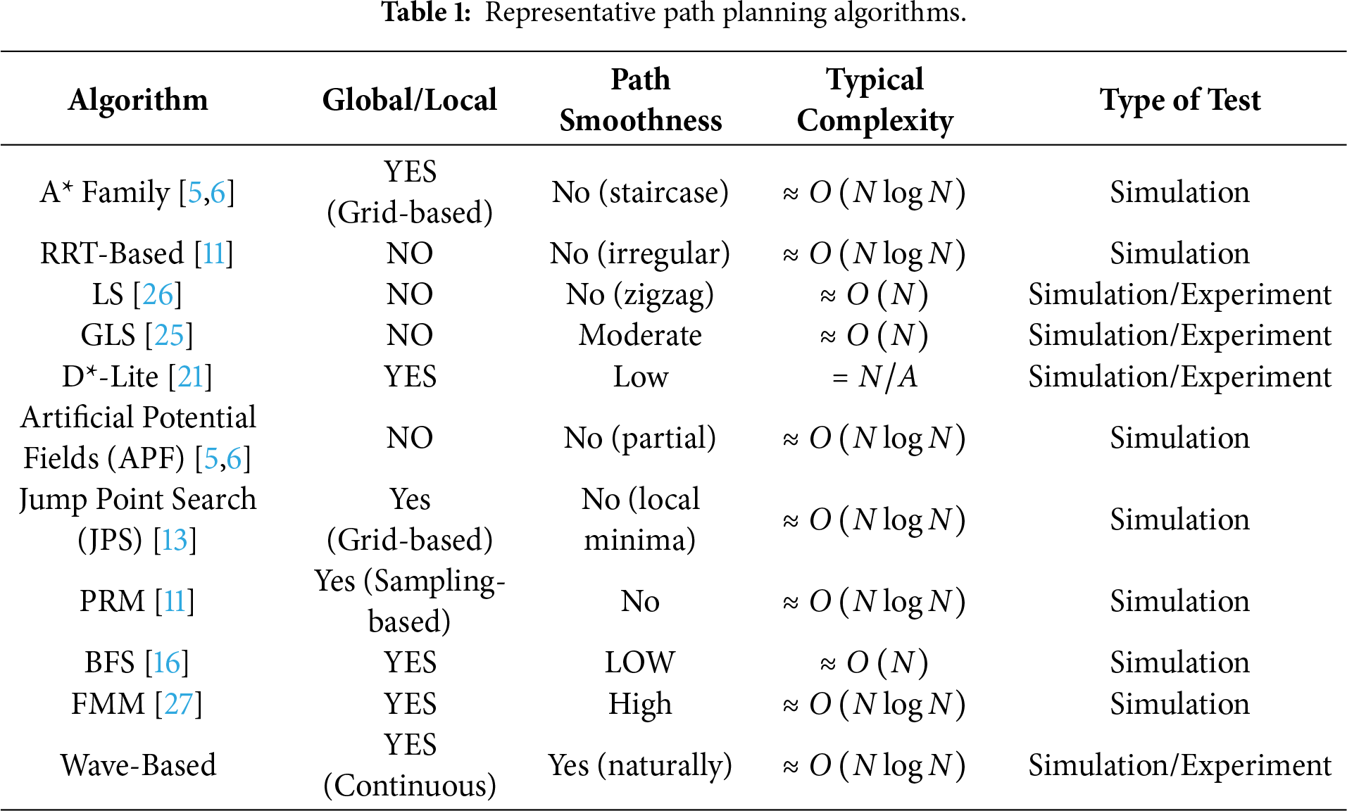
To overcome the above shortcomings, researchers have turned to wave-propagation algorithms that ensure a more global and exhaustive search of the environment. The classic wavefront (brushfire) algorithm floods the space from the start (or goal) like a BFS, ensuring all free cells are reached in increasing distance order [16]. This guarantee finding the shortest path (for uniform costs) and avoids the local minima issues of gradient-based methods. The resulting paths, however, follow the grid geometry—often involving Manhattan-like turns—and may hug obstacle boundaries (yielding low clearance). A prominent example is the Fast Marching Method (FMM), an algorithm that treats path planning as an Eikonal equation problem and efficiently computes the arrival time of a wavefront spreading across the map [17]. In robotics, FMM has been used to compute smooth, near-optimal paths on occupancy grids by simulating the expansion of a wave from the start position until it reaches the goal [18–20]. This approach shares similarities with Dijkstra’s algorithm in the way it incrementally expands a frontier, but unlike Dijkstra’s purely grid-based costs, FMM solves for continuous cost accumulations (distances or travel times) via the Eikonal update, yielding a path that is not constrained by grid direction biases moreover, because the wavefront propagation in FMM guarantees the minimal-time path before any clearance weighting; additional bias may deviate from that optimum [7,21]. Numerous works have built upon FMM’s foundation—for instance, the Fast Marching Square (FMS) variant runs FMM twice (first to create a repulsive potential field around obstacles, and second to plan on that modified cost map), resulting in paths that keep a safer clearance from obstacles [22]. By contrast, local or heuristic-driven methods—including Laser Simulator (LS) and distance-transform-based Generalized Laser Simulator (GLS)—expand incrementally and maintain agility in sparse or partially known settings [23–25]. These developments demonstrate the versatility and effectiveness of wave-based planning approaches, although they may introduce additional parameters (such as weightings for the repulsive field in FMS) that require careful tuning for different environments. Table 1 provides an overview of major path planning algorithms, contrasting their nature, path quality, typical evaluation method, complexity, and key characteristics in context. Although these existing path planning solutions have significantly advanced robotic navigation, they still face key limitations in real-world environments.

This paper is structured as follows. Section 2 details the proposed analytical wave model and its path planning formulation. Section 3 describes implementation details and validates the algorithm in simple and complex simulation scenarios and demonstrates indoor and outdoor experiments. Section 4 summarizes the main conclusions of the study.

2  Method

This section introduces the analytical two-dimensional wave equation and demonstrates how its solution underpins the proposed Wave Water Simulator (WWS). The goal is to highlight how continuous wave propagation creates a global arrival-time map that, in turn, guides path construction around static obstacles.

2.1 The Principle of Wave Water Simulator

A novel wave-based path planning framework is proposed, with its flowchart shown in Fig. 1. This framework leverages a continuous wave expansion to reveal global navigability and efficiently extract collision-free routes. First, the environment map is generated or loaded, marking obstacles and free cells. Next, a selective corridor is optionally applied to constrain wave expansions, reducing computation in large or cluttered domains. Then, the wave equation is used to derive arrival times across the corridor, reflecting each cell’s accessibility from the start node. Finally, a backtracking stage applies a cost function to preserve clearance while extracting a smooth, feasible path. This wave-centric design naturally encodes corridor effects and obstacle boundaries, producing globally consistent trajectories without relying on incremental re-planning.

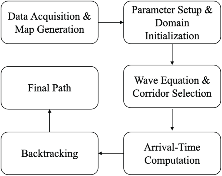
Figure 1: Overall framework for proposed Wave Water Simulator (WWS).

The Wave Water Simulator (WWS) algorithm applies the concept of wave expansion to path planning by continuously propagating a simulated wavefront from the robot’s initial position throughout the environment. As the wave evolves outward, it implicitly explores all reachable areas, indicating how a robot could navigate from the start to a goal. This wave-centric perspective avoids the pitfalls of purely heuristic methods, naturally bypassing local minima and covering the free space in an unbiased manner.

As shown in Fig. 2a, The Wave Water Simulator (WWS) algorithm applies an analytical two-dimensional wave equation to model path planning as a physical wave expansion from the robot’s start position. As the wavefront propagates outward, Dirichlet boundary conditions (U=0) are imposed at domain edges and obstacle surfaces, causing the wave amplitude to drop to zero on contact. This absorption mechanism naturally prevents the wave from crossing into invalid regions and obviates the need for separate collision detection. In open areas, the wave spreads smoothly, providing a continuous representation of arrival times for each cell; where boundaries exist, the wave simply ceases to propagate. By tracking descending arrival times from a goal back to the source, WWS directly produces a collision-free route that conforms to obstacles and domain limits.

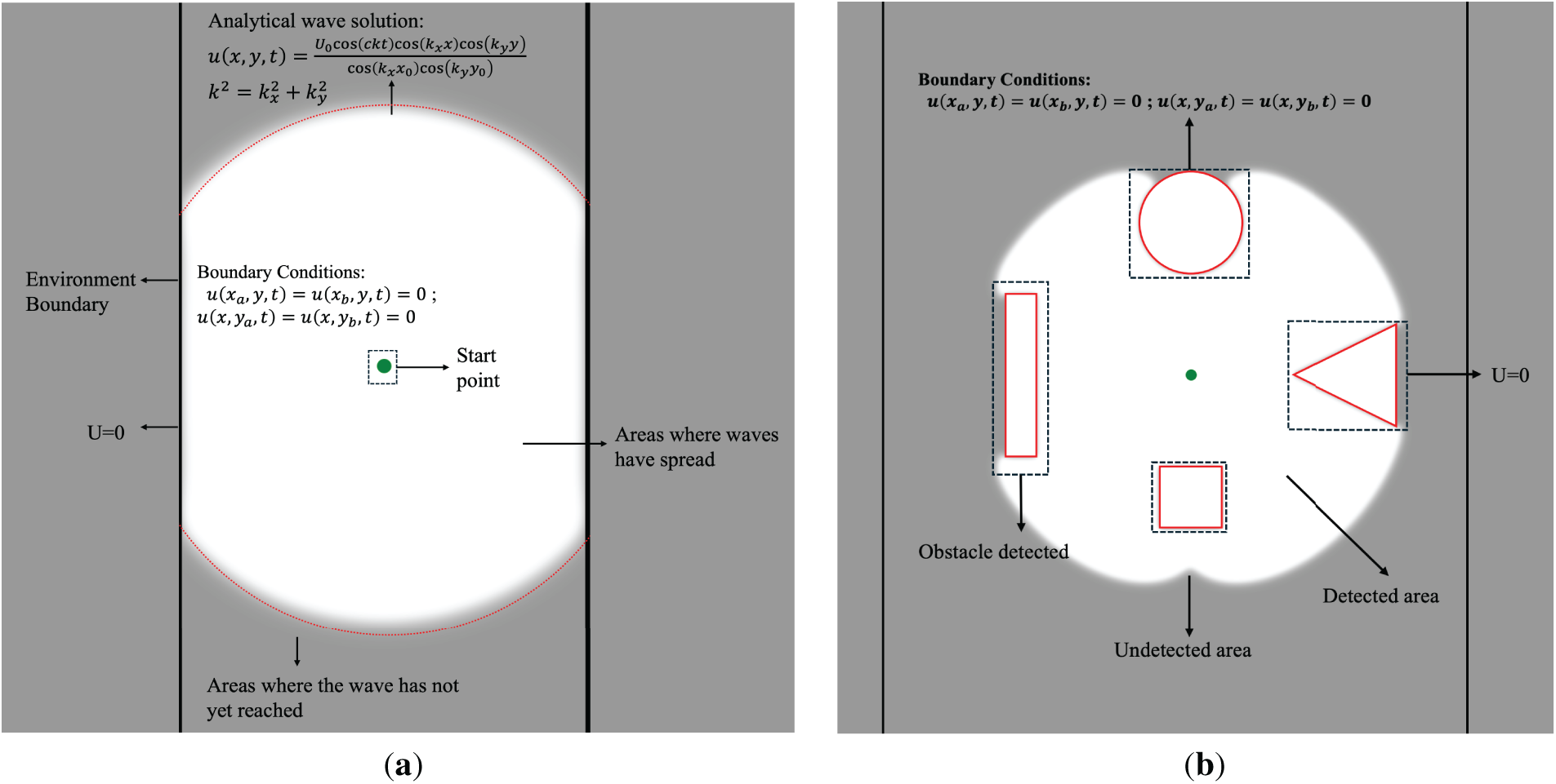
Figure 2: The principal Wave Water simulator (a) WWS spread, and boundary detect (b) WWS obstacle detection.

Fig. 2b illustrates how boundary conditions are applied in the Wave Water Simulator (WWS). Obstacles (the circular, rectangular, and triangular shapes) and the domain periphery are treated as zero-amplitude boundaries, effectively “absorbing” or blocking the wave. In the depicted scenario, the analytical solution for the two-dimensional wave equation expands smoothly from the robot’s initial position (green dot) through free space (white region), yet remains strictly confined by obstacles and outer walls. Because these boundaries enforce U=0, the wave cannot propagate into blocked cells, naturally preventing pathfinding from erroneously extending behind obstacles. This physical consistency obviates the need for separate collision detection: once an obstacle is designated as a boundary where U=0, the wave simply does not penetrate that region. As a result, WWS offers a unified framework where obstacle avoidance and global coverage are inherently incorporated into the wave equation itself, which guarantees both feasibility and smoothness of the final path.

2.2 Wave Equation Fundamentals

2.2.1 PDE-Based Wave Propagation

The two-dimensional wave equation is a well-known partial differential equation (PDE) that describes wave propagation in continuous media. In a homogeneous, bounded domain Ω⊂R2 with absorbing boundaries and obstacles, the classical form appears as:

∂2u(x,y,t)∂t2=c2(∂2u(x,y,t)∂x2+∂2u(x,y,t)∂y2)(2)

where u(x,y,t) is the wave function representing the amplitude of the wave at position (x,y) and time t, and c denotes the constant wave speed. Typical boundary conditions enforce u=0 on the domain periphery and on any obstacle surfaces, simulating perfect absorption. An initial disturbance at (x0,y0) triggers wave that expand outward until the entire reachable region is covered.

Assuming the environment is bounded within x∈[xa,xb] and y∈[ya,yb], Dirichlet boundary conditions are applied to simulate wave absorption at the boundaries and obstacles:

u(xa,y,t)=u(xb,y,t)=0(3)

u(x,ya,t)=u(x,yb,t)=0(4)

At t=0 the robot injects a unit impulse at its start location (x0,y0)

u(x,y,t)=U0δ(x−x0)δ(y−y0),u.(x,y,0)(5)

Assume u(x,y,t)=X(x)Y(y)T(t). Substituting into (2) and dividing gives:

1c2T′′T=X′′X+Y′′Y=−k2(6)

Introducing another constant −kx2:

T′′+c2k2T=0;X′′+kx2X=0;Y′′+ky2Y=0;kx2+ky2=k2(7)

kx=nπxb−xa,ky=nπyb−ya,n,m∈N+

For path planning, an analytical solution of the above PDE provides the temporal evolution of wave within Ω. The final expression for u(x,y,t) can be compactly written in the form:

u(x,y,t)=Hcos⁡(ckt)cos⁡(kxx)cos⁡(kyy)(8)

where kxand ky Ware integer-based wave numbers determined by the boundary lengths in x and y, and H encapsulates the initial amplitude U0.

Obstacles are inserted as additional boundaries, effectively zeroing out wave amplitude in those regions. Arrival times T(x,y) at which |u(x,y,t)| first surpasses a threshold δ then serve as the basis for constructing a global cost map—each location is labeled by its earliest wavefront encounter.

When implementing numerical methods to solve the wave equation, it is essential to ensure numerical stability. The Courant-Friedrichs-Lewy (CFL) condition provides a criterion for stability in finite difference methods:

cΔtΔx≤12(9)

where Δt is the time step and Δx is the spatial discretization step. Satisfying this condition prevents non-physical oscillations and ensures accurate numerical results.

2.2.2 Wave Coverage and Arrival-Time Mapping

The solution in (2) provides a continuous depiction of how the wave expands from (x0,y0). At each location (x,y) the wave amplitude u(x,y,t) eventually surpasses a chosen threshold δ, indicating that point has been “reached” by the wavefront. The arrival time T(x,y) is defined as the earliest t≥0 for |u(x,y,t)|≥δ formally:

T(x,y)=min{t≥0|u(x,y,t)|≥δ}(10)

This mapping captures global accessibility: areas near (x0,y0) exhibit small T while cells separated by obstacles or long corridors have significantly larger values.

Fig. 3a illustrates how the total area “covered” by the propagating wave evolves over continuous time according to the analytical two-dimensional wave solution. At t=0, the wave originates at the source location, and initially, only a small region around this source exhibits sufficient amplitude. As time increases, the wave expands outward in a continuous manner, surpassing a chosen amplitude threshold δ across successively larger portions of the domain. It initially rises slowly, reflecting the local nature of early propagation, then accelerates as more corridors become accessible. Eventually, the coverage begins to plateau, indicating that the wave has fully enveloped the free areas of the environment, while obstacles continue to act as absorbing boundaries.

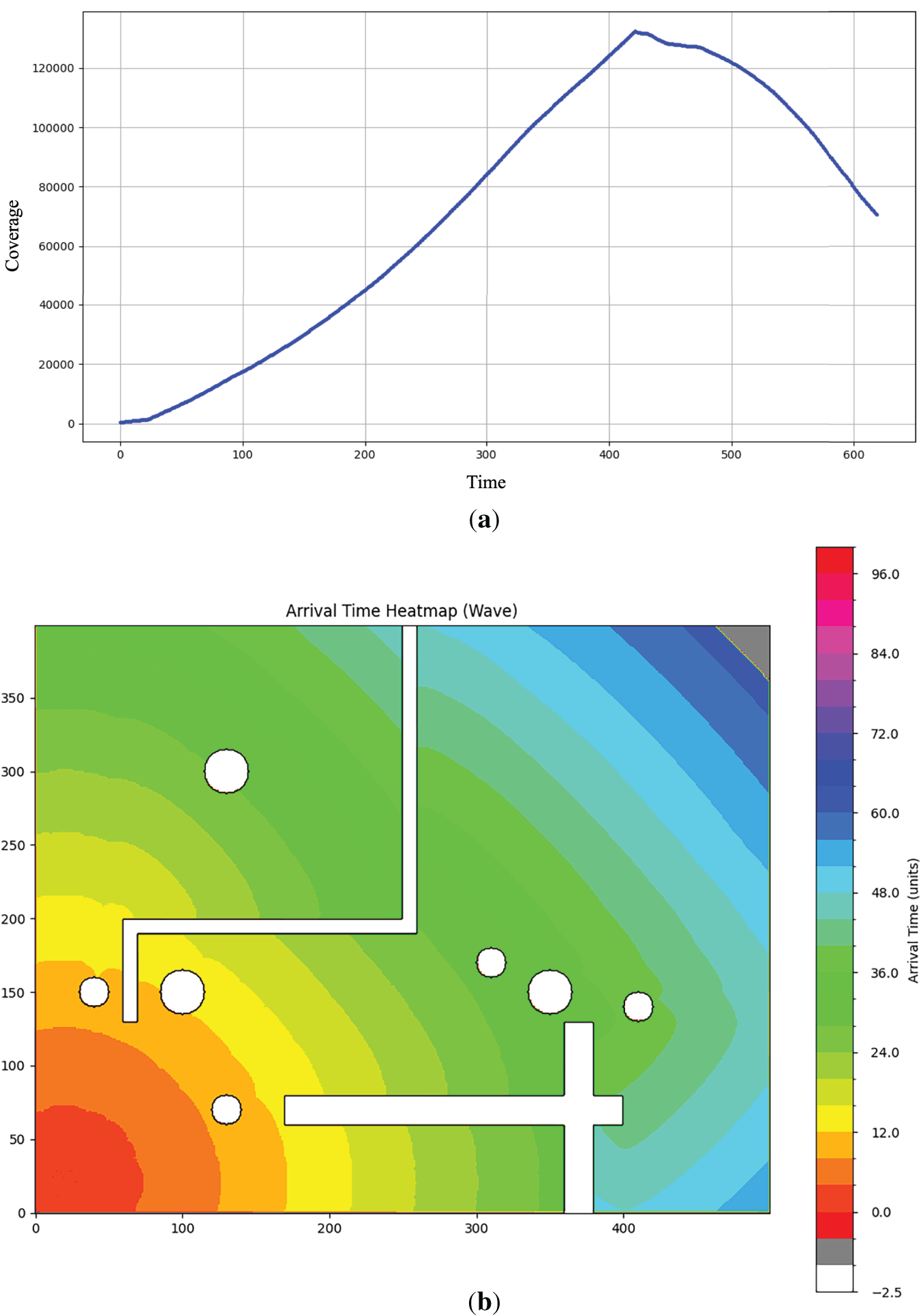
Figure 3: WWS spread illustration, (a) Wave coverage curve, (b) Arrive time heat map.

Fig. 3b offers a complementary arrival-time heatmap, again derived from the closed-form wave function. For each point (x,y) within the environment, the earliest time T(x,y) at which the wave amplitude |u(x,y,t)| crosses the threshold δ is recorded. Warmer colors (reds, oranges) correspond to shorter arrival times and thus easier accessibility from the wave source, whereas cooler colors (greens, blues) indicate cells that are reached later due to either greater distances or more complex obstacle placements. The white regions represent obstacles themselves, where wave energy is extinguished by boundary conditions, ensuring that no spurious paths are formed through invalid areas. These smoothly varying contours show natural bending of the wavefront around obstacles, demonstrating how the analytical wave solution inherently encodes corridor effects and global coverage without reliance on incremental or localized expansions.

This time map provides crucial information about the earliest time the influence from the starting point reaches any given location, which is instrumental in the subsequent path planning stages.

Once T(x,y) established throughout Ω the final path is extracted by traversing from the goal (xg,yg) back to (x0,y0) along cells with strictly decreasing arrival times. A generic neighbor (x′,y′) is deemed valid if:

T(x′,y′)<T(x,y)(11)

Ensuring that the path moves “upstream” toward the wave source. However, it is often beneficial to incorporate a cost function that penalizes obstacle proximity, ensuring safer navigation. Let D(x,y) denote the distance from (x,y) its nearest obstacle. A combined cost is then defined as:

C(x,y)=γT(x,y)+α[1D(x,y)+ε](12)

where: γ is a weighting factor that adjusts the influence of the arrival time on the cost. α is a weighting factor that adjusts the influence of the obstacle proximity on the cost. ε is a small positive constant to prevent division by zero when D(x,y) approach zero.

During backtracking, each cell’s neighbor set may include 8 adjacent positions. The path candidate (x′,y′) that yields the smallest C(x′,y′) subject to T(x′,y′)<T(x,y) is chosen at each iteration, until eventually (x0,y0) is reached. This process naturally forms a smooth, single-pass route that avoids corners and obstacles, reflecting the wave’s own continuous expansion.

2.2.3 Implementation Details

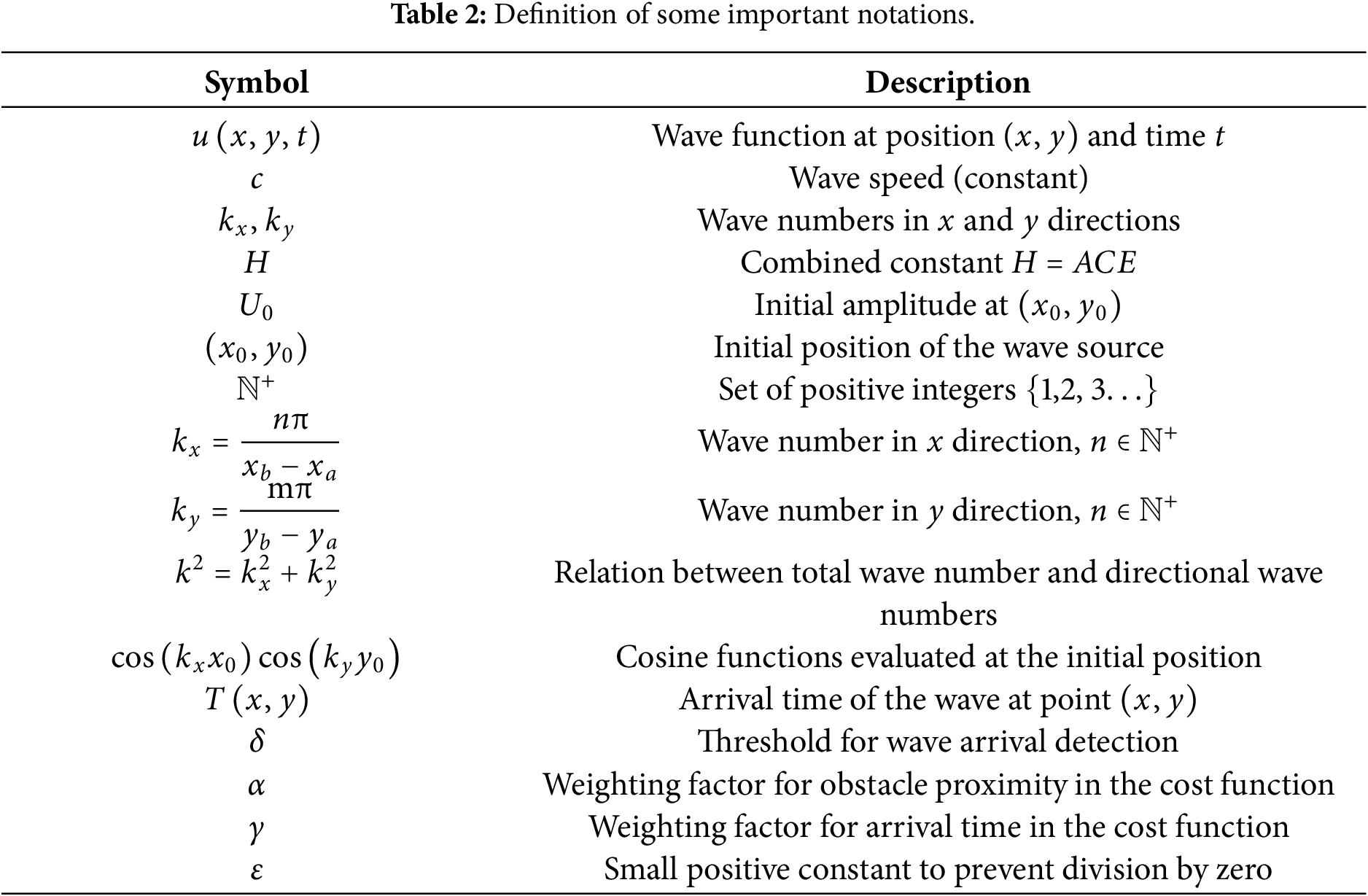
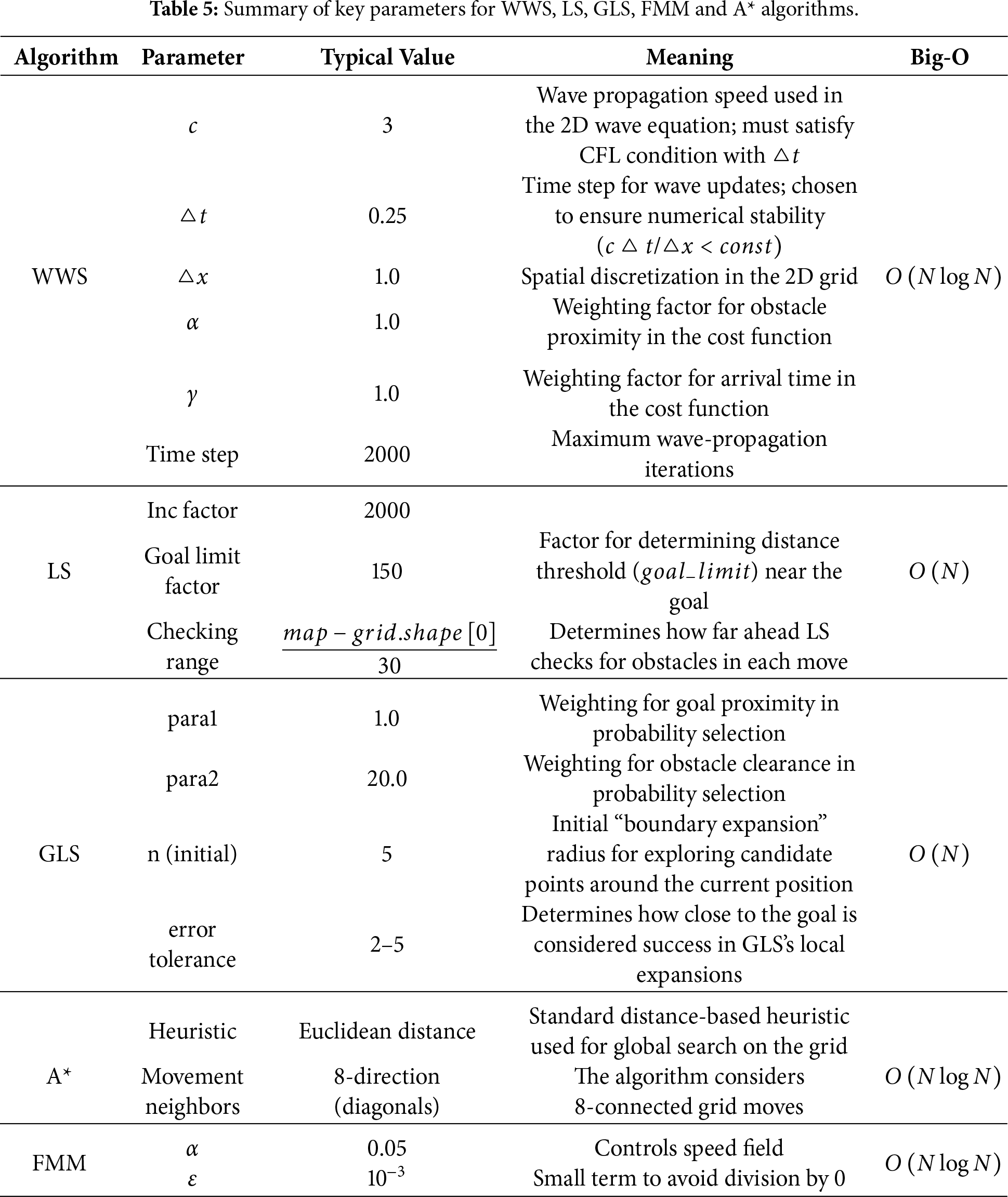
WWS requires a few critical parameters. The wave speed c is chosen as the largest value that still satisfies the Courant–Friedrichs–Lewy stability condition, Its role is to control how quickly the wavefront expands across the grid, ensuring that each cell’s arrival time is distinguishable while adhering to stability constraints [28,29]. The arrival threshold δ defines when a cell is deemed “reached”, balancing early detection against coverage gaps. During backtracking, cost weights αand γ control the trade-off between obstacle avoidance and quick arrival, useful for tuning path safety in narrow passages. Finally, an optional corridor restriction confines wave evaluation to a subregion, reducing computation in large or cluttered maps.

A summary of these main parameters and constraints appears in Table 2. Full derivations are readily found in standard references on wave phenomena, so this section only highlights key points relevant to the wave-based laser simulator proposed in this work.

In this work, the parameters—wave speed c, threshold δ, and cost-function weights α, γ—are maintained as fixed values across all experiments, both indoors and outdoors. This non-adaptive choice was guided by preliminary trials indicating that a single parameter set could provide robust performance in a variety of environments. While this approach does not automatically adjust to factors such as map scale or obstacle density, the global nature of wave expansions in WWS enables it to accommodate moderate variations without specialized tuning. We emphasize that the current study aims to demonstrate the general feasibility and effectiveness of WWS under a single, empirically chosen configuration. Nonetheless, we acknowledge that certain advanced applications—especially those with highly dynamic or drastically varying obstacle layouts—may benefit from online parameter adaptation, a direction we outline in the Conclusion.

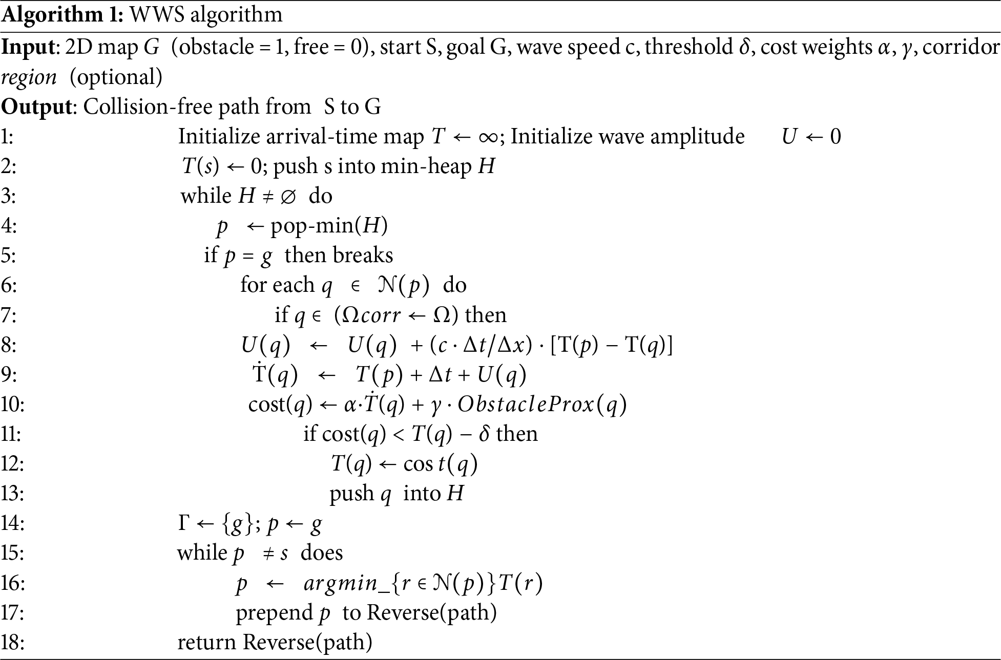
Algorithm 1 is the pseudo-code illustrating the key steps of the WWS approach under an analytical wavefront framework. It begins by defining the spatial domain and obstacle/boundary conditions, then computes the arrival-time T(x,y) for each grid cell based on the analytical wave equation solution. Once the global arrival-time map is established, a reverse-search from the goal to the start identifies the collision-free path that minimizes both travel time and obstacle proximity:

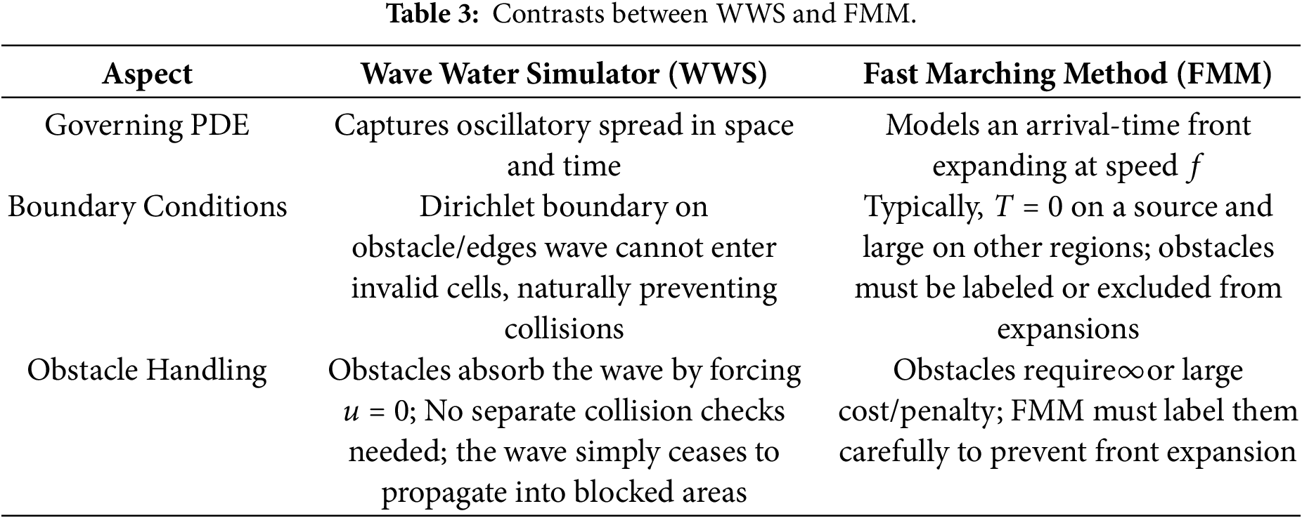
Comparison with FMM and Eikonal-Based Methods

While the wave equation underpins our Wave Water Simulator (WWS), many path planning techniques rely on the Eikonal equation, ∥∇T∥=f(x) and its fast numerical solver, the Fast-Marching Method (FMM). In FMM, one typically solves for the arrival-time T(x) of a wave or front propagating at speed f(x) This yields a globally optimal path in a continuous domain by advancing a boundary front outward. However, purely first-order PDE solutions sometimes manifest discretization artifacts or require additional boundary/obstacle labeling to ensure correct collision handling.

By contrast, WWS leverages the second-order wave equation:

∂2u(x,y,t)∂t2=c2(∂2u(x,y,t)∂x2+∂2u(x,y,t)∂y2)(13)

Together with Dirichlet boundary conditions u=0 on obstacles and domain edges. This physically motivated approach encodes obstacles as fully absorbing, preventing amplitude propagation into invalid regions without explicitly labeling them. Furthermore, the oscillatory nature of wave solutions promotes smoother curvature around corners; as the wave amplitude transitions from obstacle surfaces to free space, it avoids the “grid-sharp” expansions that sometimes arise with first-order PDE methods. Table 3 summarizes the conceptual contrasts between WWS and Eikonal-based planners, highlighting how wave-based fluctuations, direct boundary encoding, and corridor constraints distinguish WWS from FMM-like approaches.

2.2.4 Optimality and Complexity of WWS

Wave Water Simulator (WWS) adopts wave propagation akin to PDE-based planners such as FMM, it does not strictly solve the stationary Eikonal equation ∥∇T∥=f(x). Instead, WWS introduces a second-order wave equation with momentum and transient behaviors. Hence, WWS does not guarantee an exact minimal-distance path in all cases. Nevertheless, if the corridor restriction is sufficiently broad, the wave can explore the entire free space, yielding a trajectory that is empirically close to the global optimum, in narrower corridors the solution remains within 1%–2% of the global optimum in our benchmarks (in Section 3), confirming practical near-optimality.

While the Wave Water Simulator (WWS) also propagates a wavefront, it employs a binary-heap scheduler that always processes the cell with the smallest arrival time. Let Ω contain N free cells. Every cell enters the heap at most once and up to k (≤8) neighbors are relaxed, giving:

Time(WWS)=O(Nlog⁡N),Space(WWS)=O(N)(14)

If the optional corridor restriction reduces the working set from N to R cells (R ≪ N in cluttered. maps), the bound becomes O(Rlog⁡R). Back-tracking from goal to start is linear in path length L and does not alter the dominant term.

3  Results and Discussion

3.1 WWS Simulation Results Analysis

3.1.1 WWS in Simple Environment

To demonstrate the core principles of WWS, we first consider a simple 2D domain containing a single rectangular obstacle (Fig. 4). The start point (green) is placed near the lower-left corner, with the goal (red) in the upper-right region. Initially, no precomputed roadmap or heuristic is used—WWS merely propagates a wavefront from the start. As the wave expands, arrival-time contours naturally bend around the obstacle, revealing both safe corridors and areas of higher traversal cost. This obstacle interaction emerges directly from the boundary conditions, which without additional collision checks.

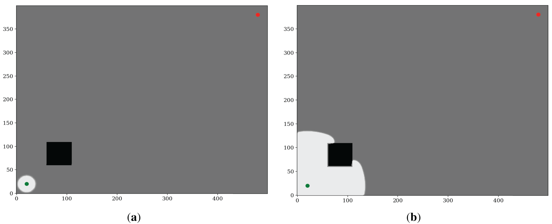
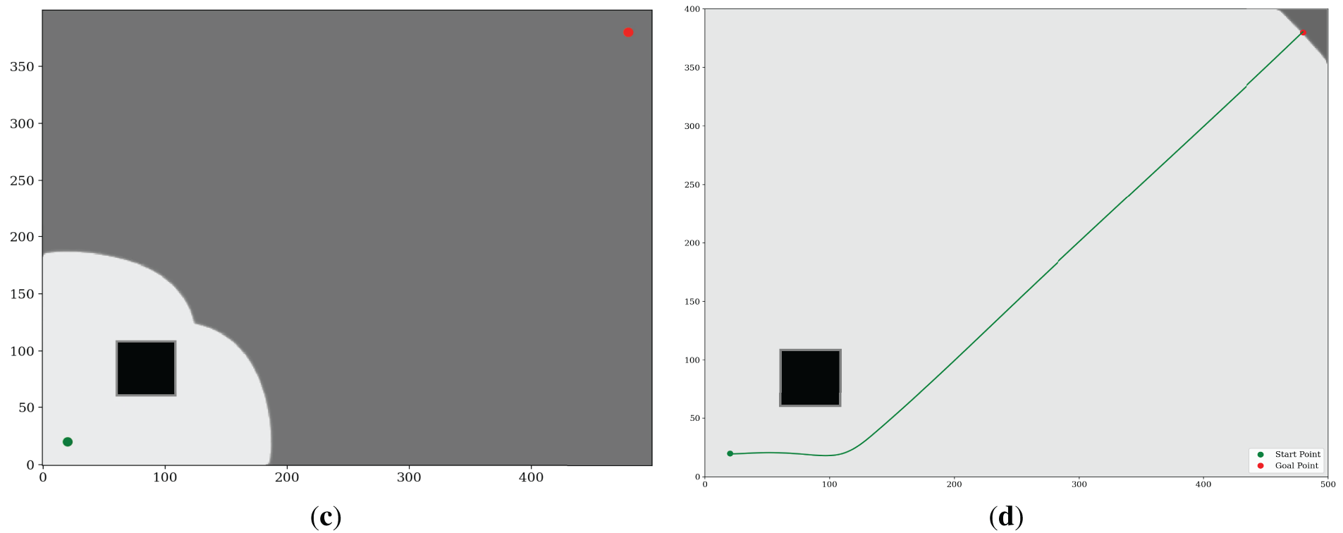
Figure 4: WWS implementation in simple environment: (a) expansion stage 1, (b) expansion stage 2, (c) expansion stage 3, (d) expansion stage 4.

Once the wavefront has covered the navigable domain, a reverse search from the goal follows cells with strictly decreasing arrival times, culminating in a collision-free path that blends efficiency and smoothness. As shown in Fig. 4, the final trajectory deftly avoids “staircase” artifacts and abrupt turns, underscoring how WWS’s global wave equation framework inherently encodes obstacle avoidance and ensures gentle curvature.

3.1.2 WWS in Complex Environment

To further test WWS beyond a single obstacle, we examined a cluttered 2D domain with multiple static obstacles of various shapes (Fig. 5). These linear barriers and circular impediments form narrow corridors, semi-enclosed passageways, and partial maze structures. Unlike local or heuristic planners susceptible to dead ends in such intricate layouts, WWS starts by globally propagating a wavefront from the start. As the wavefront evolves, arrival-time contours naturally reveal corridors and bottlenecks, offering continuous, domain-wide feedback on accessibility without incremental trial-and-error.

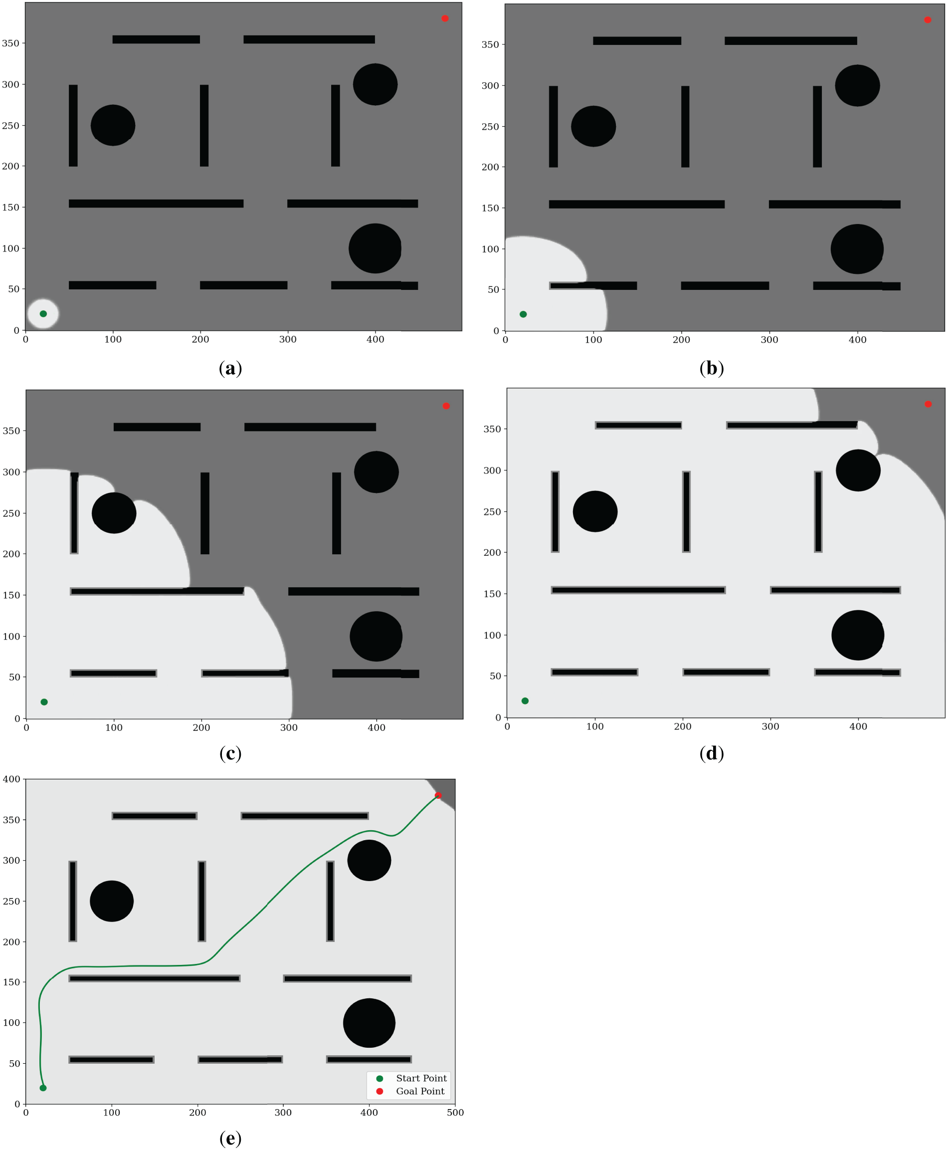
Figure 5: WWS implementation in complex environment: (a) expansion stage 1, (b) expansion stage 2, (c) expansion stage 3, (d) expansion stage 4, (e) expansion stage 5.

As wave propagation proceeds, WWS constructs a comprehensive arrival-time gradient, “lighting up” optimal routes while circumventing complex obstacles. Once all traversable cells are assigned precise times, the algorithm executes a backward traversal from the goal, following strictly decreasing arrival times. This single global expansion elegantly weaves through tight corridors and avoids local minima, eliminating the need for repeated re-planning or parametric tuning. Together with the simpler example, this scenario demonstrates WWS’s aptitude for both small-scale and maze-like environments, confirming its flexibility, global coverage, and capacity to generate naturally optimized paths.

These two sets of demonstrations—one in a simple environment and another in a considerably more complex map—collectively validate the theoretical and practical foundations of WWS. From a single obstacle to a pseudo-maze, WWS Adapts Gracefully to Complexity: The wave-based approach seamlessly scales from trivial setups to complicated geometries, without losing its capacity to discern global navigational structures. Maintains a Global Perspective: Unlike local-only methods prone to becoming stuck in dead-ends or complex corridors, WWS leverages a global arrival-time map that inherently encodes the relative difficulty of reaching any location in the domain. Produces Naturally Optimal Routes: By following decreasing arrival times from the goal to the start, WWS intrinsically finds paths that minimize travel time and respect obstacle constraints, without manually designed heuristics or extensive parameter tuning.

3.1.3 WWS in Different Complex Environment

This section demonstrates the navigation performance of the WWS algorithm in different environments, focusing on its path smoothness, obstacle avoidance capability, and adaptability to maps of varying complexity. Fig. 6 illustrates the optimal paths planned by WWS in several environments with different structures, where the start and end points are marked in green and red, respectively.

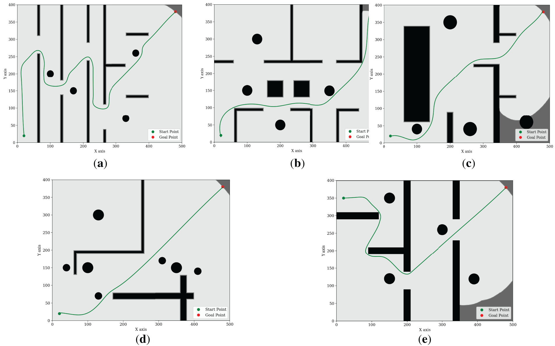
Figure 6: WWS implementation in different environment A–E: (a) environment A, (b) environment B, (c) environment C, (d) environment D, (e) environment E.

WWS exhibits strong adaptability across various environments, ensuring smooth navigation and effective obstacle avoidance. In structured obstacle environments, the algorithm accurately computes optimal paths that allow the robot to traverse narrow passages without abrupt directional changes. In maze-like environments with high obstacle density, WWS effectively avoids local optima and redundant routes while maintaining trajectory continuity. In semi-closed spaces where only specific corridors are available, WWS dynamically adjusts its path to ensure a safe distance from walls and barriers. For randomly distributed obstacles, the algorithm efficiently adapts to varying layouts, utilizing global wave propagation to avoid dead ends. In open environments, WWS generates direct and efficient paths, taking advantage of the available space for rapid goal achievement.

The simulation results confirm that WWS consistently maintains smooth trajectories and robust obstacle avoidance in diverse scenarios. The continuous wave propagation characteristic ensures that paths are both natural and efficient, enabling fluid robotic motion without excessive detours or sudden angular deviations. The algorithm’s ability to adapt to different spatial configurations highlights its potential for real-world navigation applications.

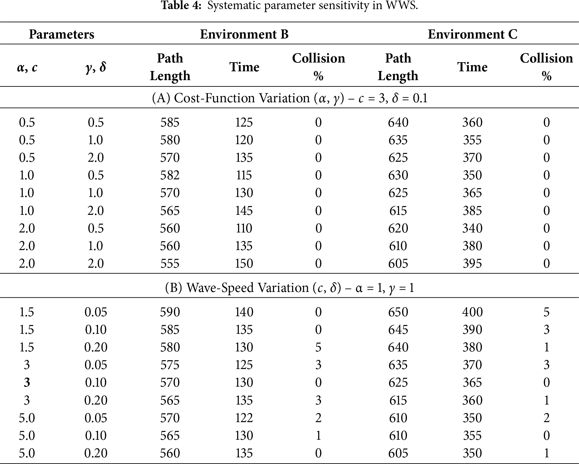
3.1.4 Systematic Parameter Sensitivity

To provide a more comprehensive understanding of how the Wave Water Simulator (WWS) algorithm behaves under different parameter settings. This investigation focuses on the four key parameters, α: obstacle proximity weight in the cost function. γ: arrival-time weight in the cost function. δ: wave detection threshold. c: wave propagation speed.

We selected three representative environments to encompass varying obstacle densities and geometric complexities, environment B, C. For each environment, the parameters are set as: α∈{0.5,1.0,2.0},γ∈{0.5,1.0,2.0},δ∈{0.05,0.1,0.2},c∈{1.5,3,5}.

Table 4 summarizes the aggregated outcomes in Environment B and Environment C for varying α, δ, c and γ. Increasing α beyond 1.0 modestly reduces path length in heavily obstructed scenes (due to stricter obstacle penalties) but can raise computation time by 5%–15%. Higher γ more strongly penalizes large arrival times, causing slightly shorter but more angular routes in some configurations. Lower thresholds δ improve detection of wave arrivals, potentially beneficial for narrow corridors. However, the algorithm sometimes requires additional updates, raising computation time by 10%–20%. Typically decreases arrival-time gradients, slightly reducing path length but having marginal effect on success rate. Overall α = 1, γ = 1, c = 3, δ = 0.1 ensure that WWS remains robust in all tested environments.

3.2 Comparison of Different Path Planning Algorithms

Simulations were performed on a machine equipped with an Intel® Core™ i7-9700 CPU @ 3.00 GHz and 16 GB RAM. All algorithms—WWS, LS, GLS, and A*—are implemented in Python 3.8 utilizing NumPy, SciPy, and Matplotlib for computations and visualizations. This common framework ensures a fair comparison.

We consider 2D grids of size approximately 500 × 400 units with △x = 1.0 and △t = 0.25 s. The wave speed c and related parameters are chosen to satisfy the CFL condition for WWS. Obstacles are represented as cells with value 1, and free space as cells with value 0. This discretization mirrors realistic operational constraints for autonomous robots navigating complex environments. Dirichlet boundary conditions enforce wave absorption at domain edges, ensuring a physically consistent wave propagation model. The start points (x0,y0) initializes the wavefront, and the goal point (xg,yg) remains within the navigable region. These conditions ensure that WWS’s arrival-time maps are always well-defined.

When selecting comparison benchmarks for this study, LS (Laser Simulator), GLS (Generalized Laser Simulator), FMM (Fast Marching Method), and A* collectively represent prominent path planning paradigms with differing trade-offs in complexity and coverage. LS employs a wave-like scanning approach that can expand globally in principle, but its reliance on directional heuristics may result in suboptimal expansions in cluttered domains. GLS extends LS by incorporating partial distance transforms or probabilistic exploration, thereby broadening coverage yet still retaining some heuristic elements. FMM adopts a continuous wavefront propagation strategy (solving the Eikonal equation) to yield smooth, near-optimal paths at the expense of higher computational overhead in larger or finer-resolution. Meanwhile, A* exemplifies a canonical discrete grid search, yielding near-optimal routes but often incurring higher computational load and producing “staircase” paths. Evaluating against these three baselines thus provides a comprehensive perspective on how the proposed algorithm compares across global coverage, heuristic guidance, computational overhead, and trajectory smoothness—key dimensions for robust, real-world robot navigation.

As shown in Table 5, algorithm parameters are chosen to reflect near-optimal conditions based on pilot studies and literature guidelines: WWS: Weighting factors α (obstacle proximity) and γ (arrival time influence) are tuned to balance safety and efficiency.GLS: Parameters (para1, para2) controlling the balance between goal proximity and obstacle avoidance follow standard published settings.LS: Uses its inherent local directional heuristics and collision checks without extensive tuning. A*: Employs a common Euclidean heuristic.

The proposed WWS (Wave Water Simulator) is compared with the baseline A*, as well as FMM (Fast Marching Method), GLS (Generalized Laser Simulator) and LS (Laser Simulator), in a series of simulated environments. Three core metrics are considered—Path Length, Computation Time, Path Smoothness—to provide a comprehensive assessment of overall performance. All performance metrics are averaged over 50 runs on diverse simulated maps to ensure statistical reliability, in accordance with best practices for rigorous evaluation in top-tier publications.

Tables 6–15 summarize the updated performance of A*, LS, GLS, FMM and WWS across 10 map configurations (A–J) in Fig. 7, this includes the percentage differences relative to A with respect to path length and planning time (Δ Path % vs. A, Δ Time % vs. A*) and their respective Big-O complexity. WWS consistently achieves shorter paths than LS, GLS, FMM and even A*, while maintaining competitive computation times. Unlike purely local methods (LS and GLS), which only examine portions of the environment, WWS adopts a more global perspective akin to A*—yet it does not exhaustively scan the entire map. Rather, WWS restricts its wavefront expansion to a corridor around the start–goal region, thus avoiding exploration of irrelevant cells far from the planned route. This selective coverage spares WWS from the high overhead often seen in A*, particularly in large or cluttered domains.

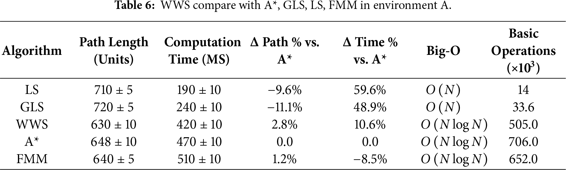
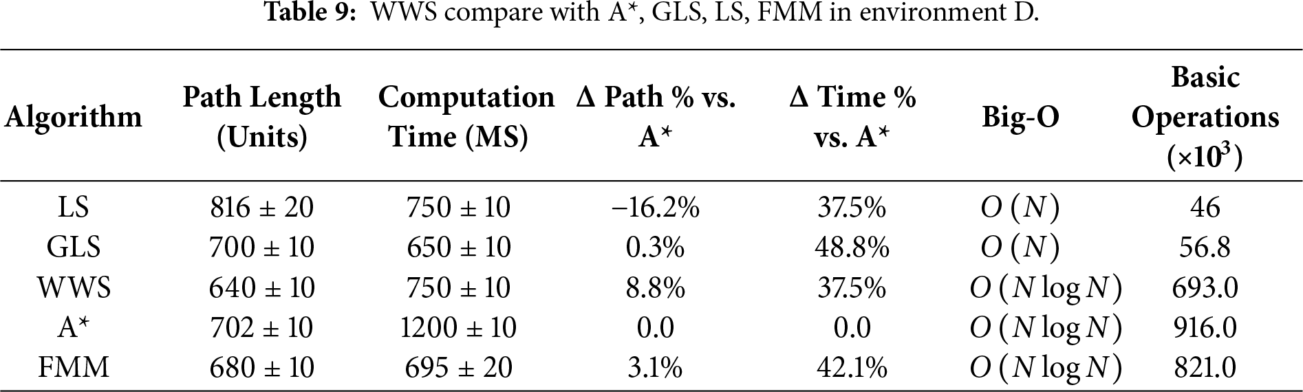
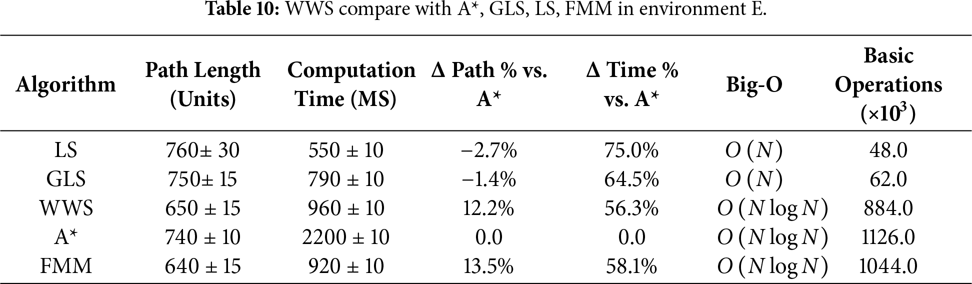
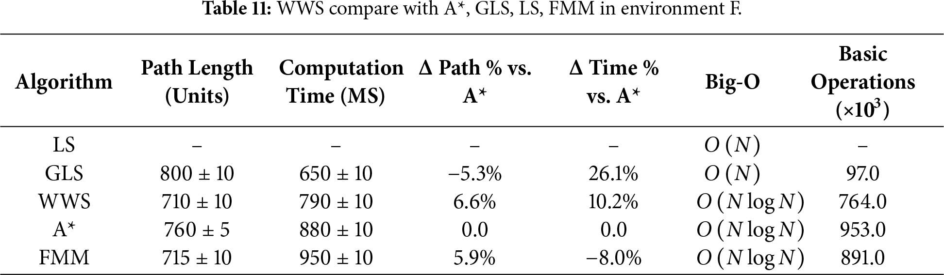
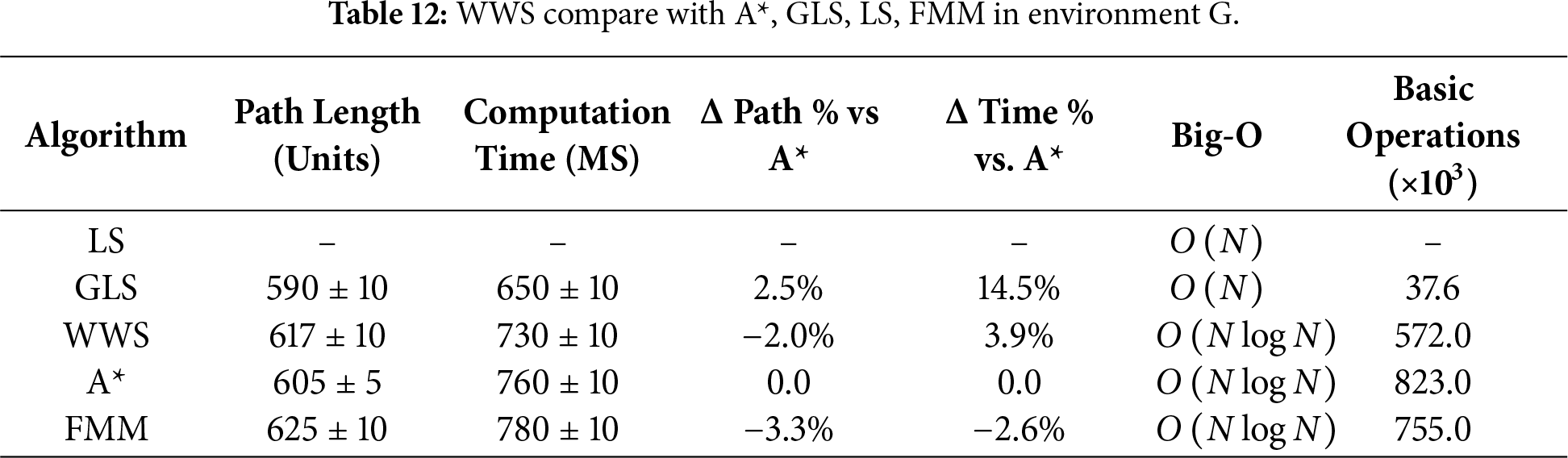
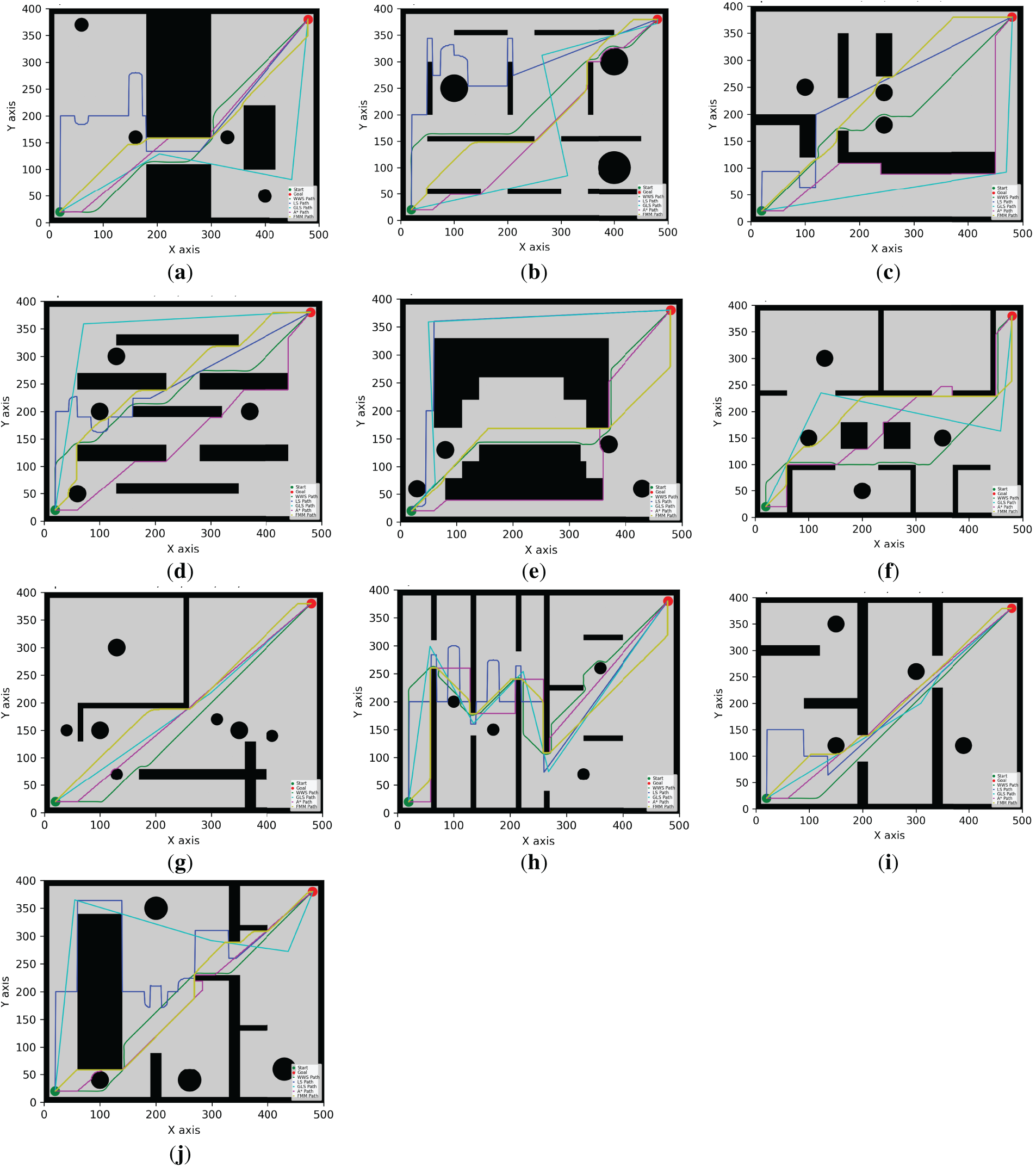
Figure 7: WWS compare with A*, GLS, LS, FMM algorithms in Environment A–J.

A clear trend in the data is that WWS not only finds near-optimal path lengths but also produces remarkably smooth trajectories. By naturally expanding wavefronts around obstacles, WWS avoids the abrupt turns and “zigzag” segments observed in many grid-based searches. In contrast, LS and GLS can generate stepwise detours due to repeated local expansions (LS even fails in maps g and f), while A* frequently yields staircase paths unless heavy post-processing is applied.

In terms of computational complexity, LS and GLS are both O(N) because they are limited to local expansion. Conversely, A*, FMM, and WWS are typically considered O(Nlog⁡N) because they require global (or semi-global) level wavefront search and sorting over a larger domain. In actual testing, A* frequently yields high overall runtime due to large-scale expansion, while WWS circumvents repetitive or redundant expansion processes because its wavefronts solely propagate within the “corridor” necessary for planning. Because each cell’s arrival time is finalized on its first (and only) visit, the wavefront expansion completes in one pass without any subsequent re-corrections or path-smoothing steps. Therefore, it is not inferior in terms of overall overhead. A comparative analysis reveals that, in a limited number of environments, WWS exhibits marginally higher computation time than FMM. However, in most scenarios, WWS demonstrates comparable or superior performance, maintaining an order of magnitude within the established parameters.

In summary, based on multiple rounds of experiments on maps A–J, WWS not only achieves comparable or superior performance to A* and FMM in terms of path quality and global feasibility, but also retains some of the computational efficiency Fig. 7a–j advantages of local methods (LS, GLS). Specifically, the shortest paths generated by WWS are slightly shorter or comparable to those of A* in most scenarios. For example, in environment E, the shortest path is approximately 12% shorter than that of A*. In environments D, F, H, and J, WWS shows an average advantage of 3%–9%. In only a few extreme scenarios (e.g., environments G and I), WWS path lengths are slightly longer than A* (approximately 2%–4%), but their smoothness is often higher. Meanwhile, about computation time, WWS frequently reduces planning overhead by 5%–15% in comparison to A*.

3.3 WWS Outdoor and Indoor Environment Test

3.3.1 Outdoor Environment Test

WWS was implemented in four distinct outdoor scenarios, designated A, B, C, and D, each characterized by varying degrees of obstacle density, road curvature, and the presence of natural or man-made structures. As shown in Fig. 8, Environment A is characterized by relative openness with sparse obstructions, while scenarios B and C introduce increasingly cluttered layouts, such as denser vegetation or narrow passageways. Environment D combines open regions with corridor-like segments, reflecting typical road networks bordered by trees or low walls. In each case, raw camera images are processed briefly (e.g., perspective alignment, threshold segmentation) to yield binary occupancy maps, where black cells represent obstructed zones and white cells are navigable.

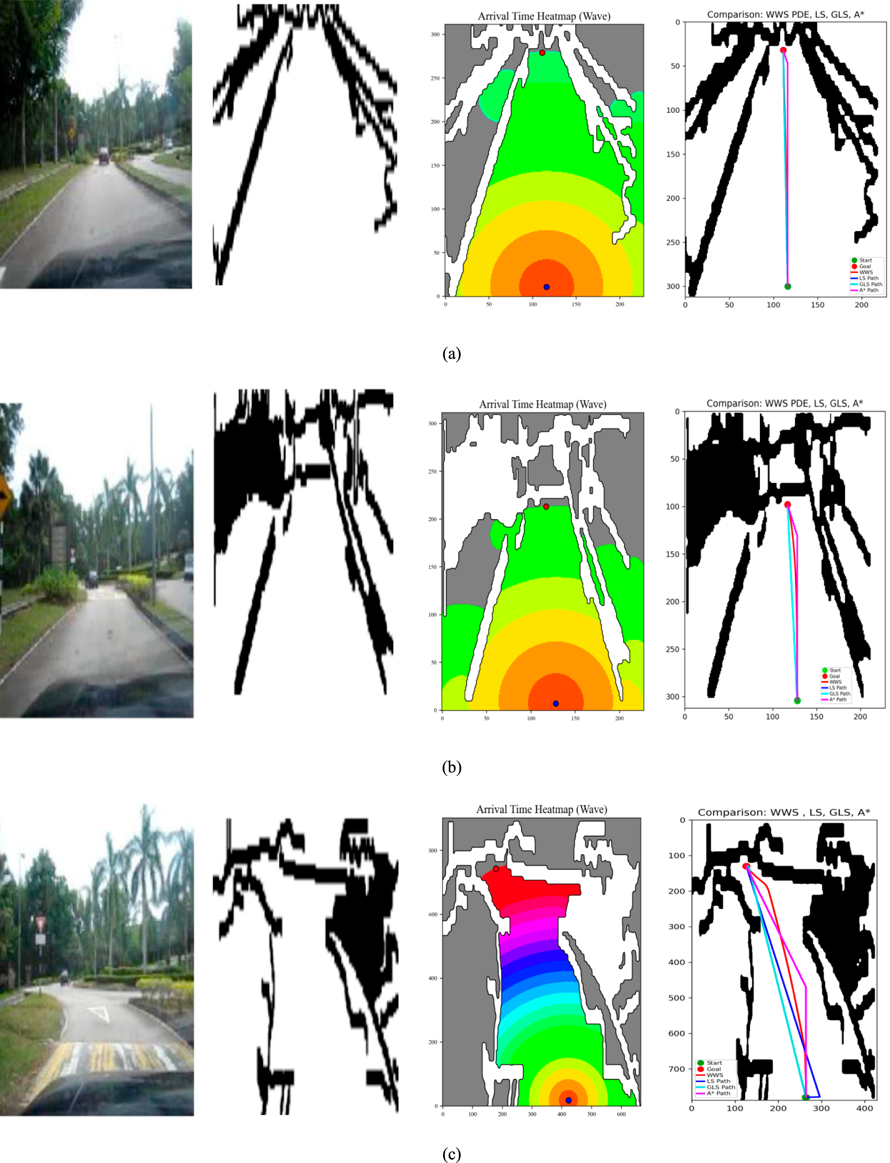
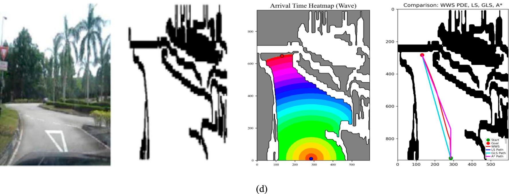
Figure 8: WWS implement in outdoor environment: (a) Outdoor environment A, (b) Outdoor environment B, (c) Outdoor environment C, (d) Outdoor environment D.

To plan a route from the start to the goal, WWS computes a wave propagation heatmap indicating how quickly each free cell is reached by the wave. The color-banded arrival-time displays reveal that warm regions (reds, oranges) denote rapid wave arrival, whereas cooler hues (greens, blues) appear in more distant or indirectly accessible areas, with obstacles remaining non-traversable (shaded or black). This heatmap visually highlights how the wave solution systematically accounts for all potential pathways around obstacles, bending around occlusions in a smooth gradient. For instance, in Environment B, the wavefront contours demonstrate gentle detours around clusters of obstacles, whereas in a tight corridor setup (e.g., C or D), the contour lines compress, revealing complex geometry. These arrival-time gradients guide the final path extraction, ensuring every feasible corridor is explored in a unified framework.

The resulting WWS paths across Environments A–D have been shown to exhibit smooth, direct navigation, even in cluttered terrain such as Environment C, where WWS avoids abrupt turns by leveraging the continuous time gradient, resulting in a path that gracefully curves around obstacles instead of making sharp angular deviations. Likewise, in corridor-like areas (Environment D), WWS blends open-area traversal with narrow corridor following, producing a coherent trajectory well suited for real vehicle motion. In comparison to earlier laser-simulator (LS) approaches, which can yield longer or more conservative routes, WWS’s wave-based formulation naturally balances obstacle clearance with minimal travel distance, achieving shorter, more efficient paths in these outdoor tests while maintaining robust collision avoidance. Compared to earlier laser-simulator approaches (LS, GLS), which can produce longer or more conservative paths due to partial expansions, WWS’s wave-based methodology systematically balances obstacle avoidance and travel distance. Although WWS’s coverage of the entire start–goal corridor can lead to higher computational complexity than LS or GLS, it remains more efficient than A*’s exhaustive global search in many cluttered or large-scale outdoor scenes.

3.3.2 Indoor Environment Test

As shown in Fig. 9, The experiments were conducted in three separate indoor laboratory settings, denoted Environments A, B, and C. Each environment featured a flat floor but varied in terms of the arrangement of obstacles. Most notably, a centrally placed tire and wooden barriers were present in Environments A and B, forcing the route to deviate. The first image in each series shows the original indoor scene, revealing how obstacles restrict the corridor or block direct travel. After this, a minimal image-processing step was applied to the scene, converting it into a binary occupancy map. This map is represented in the second image of the series, where black cells represent obstacles, and white cells denote free space.

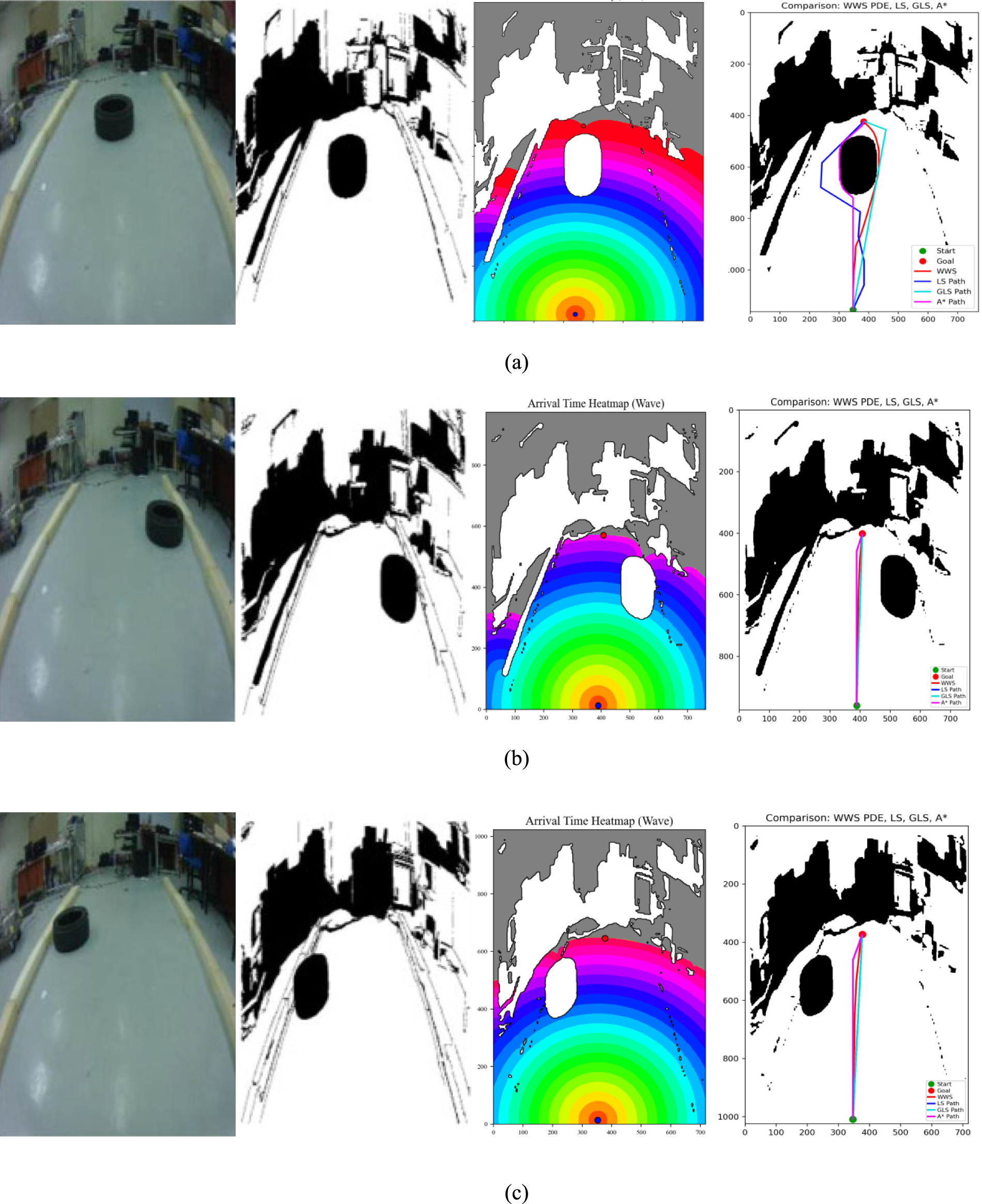
Figure 9: WWS implementation Indoor Environment: (a) Indoor environment A, (b) Indoor environment B, (c) Indoor environment C.

Following the formation of the occupancy map, the WWS algorithm calculates an arrival-time heatmap (third image), illustrating the propagation of a wave from the robot’s initial position (or goal) and its subsequent trajectory around obstacles. Each colored band in the heatmap denotes the time (or cost) required to reach that specific region. In instances where obstacles impede direct lines of travel, the wavefront curves around the obstructions, resulting in elevated arrival-time zones behind the occluding objects. This process ensures that WWS exhaustively accounts for every navigable corridor, even narrow passages. In the fourth image, the final WWS path is obtained by tracing a sequence of cells with strictly decreasing arrival times, producing a smooth, arc-like trajectory around the central tire or wooden barriers without abrupt angular turns.

In practice, WWS’s continuous wave-propagation paradigm fosters both comprehensive route exploration and high path smoothness, even in tight corridors. By expanding over the entire corridor region connecting start and goal, WWS can thoroughly map each free cell’s accessibility. This global perspective is akin to A* in that it scans a significant portion of the grid; however, WWS restricts its search to a corridor around the start–goal line, preventing a full-map scan. Consequently, WWS tends to exhibit greater computational cost than purely local methods (LS, GLS), which only sample or locally expand around the current robot location. Meanwhile, A* often has the highest overall complexity due to an exhaustive search across the entire occupancy map.

Overall, the indoor results confirm that WWS delivers high-quality navigation—a global coverage ensures no corridor is missed, while the wave-based approach gives smoother turns. Although WWS’s corridor-wide scanning increases computational burden compared to LS and GLS, it typically remains more efficient than A* in cluttered or large testbeds. Meanwhile, methods like LS, GLS, and A* are prone to “Z”-shaped or jagged trajectories, especially in obstacle-rich domains, unless extensive smoothing is applied post hoc. Hence, these findings underscore that WWS, despite its somewhat larger wave expansion, achieves shorter and smoother paths with practical computational requirements—an appealing combination for real-world robotic navigation in laboratory-scale indoor environments.

4  Conclusion

This paper presented a Wave Water Simulator (WWS) path planning algorithm that unifies global wave equation modeling with selective corridor expansion, achieving efficient and smooth navigation for autonomous robotic systems. Through comprehensive simulations and real-world tests—covering both cluttered indoor scenarios and wide-open outdoor spaces—the proposed method demonstrated consistent advantages in terms of path length reduction, smoothness, and computational cost over several established approaches. The primary conclusions are outlined as follows.

1.    The proposed WWS path planning model effectively alleviates the “staircase” or piecewise-linear artifacts observed in discrete grid-based methods. The integrated wave equation formulation promotes a naturally curved, collision-free trajectory, reducing extraneous turning angles. Across multiple test environments, compared to A*, WWS consistently achieved 2%–13% shorter path lengths, reduced planning overhead by 5%–15% in computation time while preserving—or even improving—obstacle clearance., while preserving—or even improving—obstacle clearance.

2.    By selectively confining the wave expansion to feasible corridors, WWS significantly reduces runtime and computational overhead without sacrificing global coverage. Even in cluttered maps with narrow corridors, WWS maintained real-time or near-real-time performance, minimizing re-planning cycles often required by purely heuristic or local approaches.

3.    Extensive experiments confirmed the versatility of WWS in different obstacle distributions, ranging from simple layouts to complex maze-like maps. The algorithm seamlessly adapts to various map scales and resolutions without extensive parameter tuning. This generality underscores WWS’s potential for deployment in a broad class of robotics applications, from warehouse robots to field-based autonomous vehicles.

Despite its demonstrated effectiveness, the present version of WWS employs fixed parameters (wave speed c, threshold δ, and cost-function weights α, γ) for all experiments. Our results show that these fixed values suffice across multiple indoor and outdoor tasks, suggesting a notable degree of inherent robustness. Nevertheless, we acknowledge the advantages of a partially or fully adaptive framework. Real-time adjustments to c, α, or corridor restrictions could enhance computational efficiency in large, sparsely populated environments, while selectively increasing α might provide safer clearance in densely obstructed areas. Consequently, incorporating an automated parameter-tuning mechanism—for instance, via rule-based heuristics or machine learning—represents a promising avenue for future research. Such a module could dynamically monitor environmental changes (e.g., obstacle density, sensor noise) and update critical parameters on the fly, thereby extending WWS’s versatility to real-time, unpredictable missions.

The proposed WWS offers a practical, high-accuracy, and high-efficiency path-planning solution by capitalizing on a physically motivated wave expansion while selectively restricting coverage to critical areas. Its consistent performance in both simulation and real-world tests positions WWS as a promising new benchmark for global yet computationally feasible robotic navigation. Future work will explore two complementary directions: (1) dynamic-obstacle and multi-robot scenarios, where real-time wavefront updates and distributed PDE solvers will preserve robustness in ever-changing environments; and (2) adaptive parameter tuning, in which reinforcement-learning or Bayesian-optimization layers automatically adjust wave speed c, threshold δ, and cost-weight factors (α, γ) to match local map density or mission priorities on-the-fly, further enhancing WWS’s versatility and autonomy.

Acknowledgement: Not applicable.

Funding Statement: Authors would like to thank University of Malaya and Ministry of High Education-Malaysia for supporting this work under research grant FRGS/1/2023/TK10/UM/02/3 and GPF020A-2023.

Author Contributions: Hui Chen: conceptualization, methodology, software, writing—original draft, investigation, validation, visualization; Mohammed A. H. Ali: conceptualization, supervision, methodology, writing—review & editing, validation, funding acquisition; Bushroa Abd Razak: supervision, writing—review & editing; Zhenya Wang: writing—review & editing; Yusoff Nukman: supervision, writing—review & editing; Shikai Zhang: writing—review & editing; Zhiwei Huang: writing—review & editing; Ligang Yao: writing—review & editing; Mohammad Alkhedher: funding acquisition, writing—review & editing. All authors reviewed and approved the final version of the manuscript.

Availability of Data and Materials: The authors do not have permission to share data.

Ethics Approval: Not applicable.

Conflicts of Interest: The authors declare no conflicts of interest.

References

1. Desouza GN, Kak AC. Vision for mobile robot navigation: a survey. IEEE Trans Pattern Anal Mach Intell. 2002;24(2):237–67. doi:10.1109/34.982903. [Google Scholar] [CrossRef]

2. Hornung A, Phillips M, Jones EG, Bennewitz M, Likhachev M, Chitta S. Navigation in three-dimensional cluttered environments for mobile manipulation. In: Proceedings of the 2012 IEEE International Conference on Robotics and Automation; 2012 May 14–18; Paul, MN, USA. p. 423–9. [Google Scholar]

3. Hoy M, Matveev AS, Savkin AV. Algorithms for collision-free navigation of mobile robots in complex cluttered environments: a survey. Robotica. 2015;33(3):463–97. doi:10.1017/s0263574714000289. [Google Scholar] [CrossRef]

4. Li H, Savkin AV. An algorithm for safe navigation of mobile robots by a sensor network in dynamic cluttered industrial environments. Robot Comput Integr Manuf. 2018;54:65–82. doi:10.1016/j.rcim.2018.05.008. [Google Scholar] [CrossRef]

5. Abdel-Rahman AS, Zahran S, Elnaghi BE, Nafea SF. Enhanced hybrid path planning algorithm based on APF and a-star. Int Arch Photogramm Remote Sens Spat Inf Sci. 2023;48(1):867–73. doi:10.5194/isprs-archives-XLVIII-1-W2-2023-867-2023. [Google Scholar] [CrossRef]

6. Xi W, Lin J, Shao Z. Path planning of mobile robot based on improved PRM and APF. Meas Control. 2025;58(8):979–95. doi:10.1177/00202940241291282. [Google Scholar] [CrossRef]

7. Jin J, Zhang Y, Zhou Z, Jin M, Yang X, Hu F. Conflict-based search with D* lite algorithm for robot path planning in unknown dynamic environments. Comput Electr Eng. 2023;105:108473. doi:10.1016/j.compeleceng.2022.108473. [Google Scholar] [CrossRef]

8. Yu J, Yang M, Zhao Z, Wang X, Bai Y, Wu J, et al. Path planning of unmanned surface vessel in an unknown environment based on improved D*Lite algorithm. Ocean Eng. 2022;266:112873. doi:10.1016/j.oceaneng.2022.112873. [Google Scholar] [CrossRef]

9. Guo H, Li Y, Wang H, Wang C, Zhang J, Wang T, et al. Path planning of greenhouse electric crawler tractor based on the improved A* and DWA algorithms. Comput Electron Agric. 2024;227(1):109596. doi:10.1016/j.compag.2024.109596. [Google Scholar] [CrossRef]

10. Wang H, Lou S, Jing J, Wang Y, Liu W, Liu T. The EBS-A* algorithm: an improved A* algorithm for path planning. PLoS One. 2022;17(2):e0263841. doi:10.1371/journal.pone.0263841. [Google Scholar] [PubMed] [CrossRef]

11. Tang H, Zhu Q, Shang E, Dai B, Hu C. A reference path guided RRT* method for the local path planning of UGVs. In: Proceedings of the 2020 39th Chinese Control Conference (CCC); 2020 Jul 27–29; Shenyang, China. p. 3904–9. [Google Scholar]

12. Zhou X, Wang X, Xie Z, Gao J, Li F, Gu X. A Collision-free path planning approach based on rule guided lazy-PRM with repulsion field for gantry welding robots. Robot Auton Syst. 2024;174:104633. doi:10.1016/j.robot.2024.104633. [Google Scholar] [CrossRef]

13. Huang J, Wu Y, Lin X. Smooth JPS path planning and trajectory optimization method of mobile robot. Trans Chin Soc Agric Mach. 2021;52(2):22–30. [Google Scholar]

14. Sánchez-Ibáñez JR, Pérez-Del-Pulgar CJ, García-Cerezo A. Path planning for autonomous mobile robots: a review. Sensors. 2021;21(23):7898. doi:10.3390/s21237898. [Google Scholar] [PubMed] [CrossRef]

15. Zhang W, Xu G, Song Y, Wang Y. An obstacle avoidance strategy for complex obstacles based on artificial potential field method. J Field Robot. 2023;40(5):1231–44. doi:10.1002/rob.22183. [Google Scholar] [CrossRef]

16. Ugwoke KC, Nnanna NA, Abdullahi SE. Simulation-based review of classical, heuristic, and metaheuristic path planning algorithms. Sci Rep. 2025;15(1):12643. doi:10.1038/s41598-025-96614-2. [Google Scholar] [PubMed] [CrossRef]

17. Telea A. An image inpainting technique based on the fast marching method. J Graph Tools. 2004;9(1):23–34. doi:10.1080/10867651.2004.10487596. [Google Scholar] [CrossRef]

18. Danielmeier L, Seitz S, Barz I, Hartmann P, Hartmann M, Moormann D. Modified constrained wavefront expansion path planning algorithm for Tilt-Wing UAV. In: Proceedings of the 2022 International Conference on Unmanned Aircraft Systems (ICUAS); 2022 Jun 21–24; Dubrovnik, Croatia. p. 676–85. [Google Scholar]

19. Ding B, Xin Z, Yin H. Global smooth solutions of 2D quasilinear wave equations with higher-order null conditions and short pulse initial data. Sci China Math. 2025:1–70. doi:10.1007/s11425-024-2405-4. [Google Scholar] [CrossRef]

20. Ibrahim I, Gillis J, Decré W, Swevers J. Exact wavefront propagation for globally optimal one-to-all path planning on 2D Cartesian grids. IEEE Robot Autom Lett. 2024;9(11):9431–7. doi:10.1109/LRA.2024.3460409. [Google Scholar] [CrossRef]

21. Al-Mutib K, AlSulaiman M, Emaduddin M, Ramdane H, Mattar E. D* Lite based real-time multi-agent path planning in dynamic environments. In: Proceedings of the International Conference on Computational Intelligence, Modelling and Simulation (CSSIM); 2011 Sep 20–22; Washington, DC, USA. p. 170–4. [Google Scholar]

22. Mandava RK, Mrudul K, Vundavilli PR. Dynamic motion planning algorithm for a biped robot using fast marching method hybridized with regression search. Acta Polytech Hung. 2019;16:189–208. [Google Scholar]

23. Ali MA, Mailah M, Hing TH. Implementation of laser simulator search graph for detection and path planning in roundabout environments. WSEAS Trans Signal Process. 2014;10:118–26. [Google Scholar]

24. Ali MAH, Mekhilef S, Yusoff N, Razak BA. Laser simulator logic: a novel inference system for highly overlapping of linguistic variable in membership functions. J King Saud Univ Comput Inf Sci. 2022;34(10):8019–40. doi:10.1016/j.jksuci.2022.07.017. [Google Scholar] [CrossRef]

25. Muhammad A, Ali MAH, Turaev S, Abdulghafor R, Shanono IH, Alzaid Z, et al. A generalized laser simulator algorithm for mobile robot path planning with obstacle avoidance. Sensors. 2022;22(21):8177. doi:10.3390/s22218177. [Google Scholar] [PubMed] [CrossRef]

26. Ali MA, Mailah M. Laser simulator: a novel search graph-based path planning approach. Int J Adv Rob Syst. 2018;15(5):172988141880472. doi:10.1177/1729881418804726. [Google Scholar] [CrossRef]

27. Mirebeau JM, Portegies J. Hamiltonian fast marching: a numerical solver for anisotropic and non-holonomic eikonal PDEs. Image Process Line. 2019;9:47–93. doi:10.5201/ipol.2019.227. [Google Scholar] [CrossRef]

28. Tryggvason G, Scardovelli R, Zaleski S. Direct numerical simulations of gas-liquid multiphase flows. Cambridge, UK: Cambridge University Press; 2011. [Google Scholar]

29. Sethian JA, University of California, Berkeley. Level set methods and fast marching methods. 2nd ed. Cambridge, UK: Cambridge University Press; 1999. [Google Scholar]