Optimizing RPL Routing Using Tabu Search to Improve Link Stability and Energy Consumption in IoT Networks

1  Introduction

The Internet of Things (IoT) allows devices to communicate and interact, creating a seamless connection between the physical and digital worlds. However, deploying IoT networks presents several challenges, especially regarding energy efficiency and link stability [1–3]. These factors are critical for maintaining reliable communication in environments with limited resources and energy-constrained nodes. The RPL protocol provides a flexible and efficient routing mechanism to address these issues [4,5]. Nevertheless, the dynamic nature of IoT environments can lead to suboptimal routing decisions, which increase energy consumption, reduce connection reliability, and lower overall network performance.

Various optimisation techniques have been investigated to improve the efficiency of the RPL protocol and address these challenges [6–8]. TS is a robust metaheuristic algorithm that effectively navigates the complex search space related to routing optimisation [9–11]. TS is capable of escaping local minimum and converging towards a global optimum by systematically exploring potential solutions while using a Tabu List to avoid cycles [12]. This document presents a new methodology for optimizing RPL routing through the application of TS, with the objectives of minimizing energy consumption, enhancing link stability, and prolonging network lifespan.

In this context, the integration of advanced simulation and optimisation techniques is essential for enhancing the performance of IoT networks. These methods facilitate the real-time assessment of routing configurations and network behaviours across different conditions, reducing the risks associated with direct physical interventions. A technique that can be employed is the utilisation of a digital twin, which serves as a virtual model of the IoT system, to facilitate predictive analysis and enhance informed decision-making [13]. Our work builds on this foundation by exploring the potential of TS-based optimisation to improve the resilience and energy efficiency of large-scale IoT environments. Our approach introduces a composite cost function that incorporates several critical parameters, including Residual Energy, Transmission Energy, Distance to the Sink, HC, ETX, and LSR. By integrating these factors, the proposed method identifies the most efficient and reliable routes within the network. Simulation results demonstrate that the optimization achieves significant improvements in key performance metrics. This study contributes to ongoing efforts to enhance IoT network performance by providing a solution that is both scalable and adaptable to the evolving requirements of IoT environments.

RPL organises LLN nodes into a Destination-Oriented Directed Acyclic Graph (DODAG) whose topology is optimised locally through objective functions (OFs). The default OF0 employs HC only; several successors combine two or three metrics, but most still rely on greedy one-shot decisions that ignore network-wide side-effects. Meta-heuristics such as TS offer a principled way to navigate the global search space at affordable CPU cost. The fundamental limitation of existing RPL variants (OF0, MRHOF [14]) is their reliance on single or dual metrics, leading to suboptimal trade-offs. TABURPL employs Tabu Search to navigate the complex solution space where these objectives conflict.

Therefore, problem statement and optimization objectives are; TABURPL tries to solve the multi-objective optimization problem by focusing on five main goals at the same time. First, it aims to minimize energy consumption, which helps to extend the network lifetime. Second, it seeks to maximize the packet delivery ratio to ensure reliable network performance. Third, it aims to minimize end-to-end delay, which is essential for supporting time-sensitive applications. Fourth, it focuses on maximizing link stability in order to prevent route oscillations. Finally, it works on minimizing control overhead to preserve bandwidth.

The remainder of this paper is organized as follows: Section 2 reviews recent advances in RPL optimization, with particular emphasis on multi-metric and AI-based approaches. Section 3 introduces the proposed TABURPL protocol. It describes the TS-based mechanism, the composite cost function, metric normalization, and weight calibration. This section also presents the network model, explains the calculation of the link stability metric, and evaluates the additional control overhead. Section 4 details the simulation setup, the performance metrics used, and the comparative results across different network sizes and traffic scenarios. Finally, Section 5 provides the conclusion and outlines directions for future work.

2  Related Work

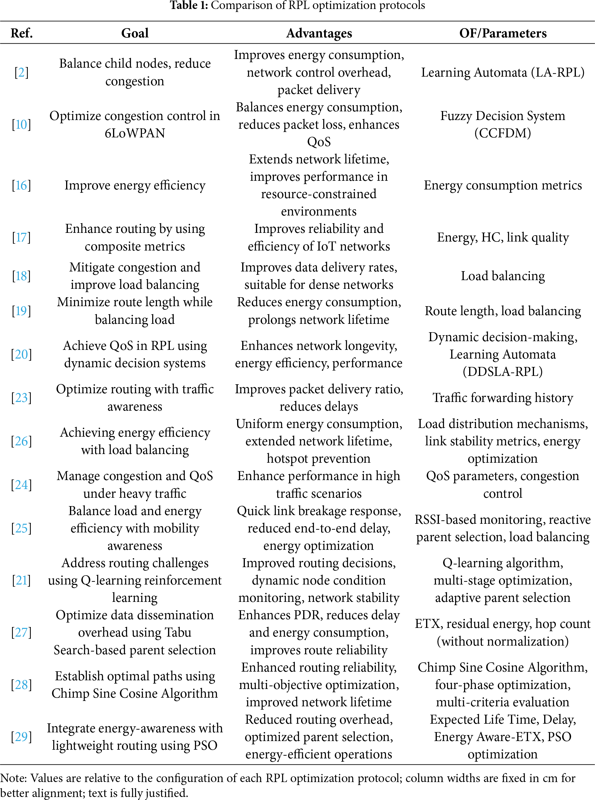
Research on RPL optimization has evolved in several phases, each tackling certain weaknesses of the standard OF0 and MRHOF approaches. In this section, we review the main strategies proposed in the literature, show how different works relate to each other, and point out the gap that TABURPL aims to fill.

2.1 Traditional Single- and Dual-Metric Approaches

The standard RPL protocol defines two primary objective functions: OF0 [15], which uses hop count as the sole routing metric, and MRHOF [13], which employs a rank-based approach combining hop count with link quality (ETX). While MRHOF represents an improvement over OF0 by incorporating link reliability, both approaches remain limited in their ability to address the multifaceted challenges of IoT routing. The first attempts to optimize RPL extended the simple hop count metric by adding energy considerations. For instance, Touzene et al. [16] suggested an energy-aware objective function that takes energy consumption into account during routing, which helps prolong the network lifetime in constrained environments. Their results indicated that even a single additional metric can improve performance compared to OF0, although such approaches are naturally limited by the trade-offs of optimizing only one extra factor.

Following this idea, Mishra et al. [17] proposed Eha-RPL, a system that combines energy, hop count, and link quality metrics in a composite objective function. This dual-metric approach performed better than single-metric methods, improving both reliability and efficiency. However, its effectiveness was hindered by the lack of systematic weight tuning and metric normalization. These early studies show that while combining metrics can help, balancing them without a structured framework remains a challenge.

2.2 Load-Balancing and Congestion-Management Solutions

It soon became clear that energy efficiency alone was not enough, especially for dense IoT networks. This led researchers to focus on load balancing and congestion control. Rana et al. [18] introduced the Enhanced Balancing Objective Function (EBOF), which aims to distribute traffic more evenly to reduce congestion and increase delivery rates. Similarly, Seyfollahi and Ghaffari [19] proposed a lightweight method that shortens routes while spreading the traffic load across nodes, thus saving energy and avoiding overused nodes.

Homaei et al. contributed two notable approaches in this area. Their LA-RPL method [2] uses Learning Automata to dynamically balance child nodes and reduce congestion through distributed data aggregation. Later, their CCFDM approach [10] applied a fuzzy decision system to 6LoWPAN protocols, controlling congestion by distributing traffic intelligently and using back-pressure mechanisms to detect problems quickly. Moving from static load balancing to these dynamic approaches was an important step forward, although these methods mostly react to congestion rather than anticipate it.

2.3 AI and Machine Learning Integration

The use of AI and ML in RPL allows more adaptive routing. Homaei et al. [20] proposed DDSLA-RPL, using Learning Automata to select parents based on hop count, link quality, and energy. It can change the weight of these metrics dynamically, showing AI’s potential for flexible RPL optimization. Reinforcement learning is also applied. Zahedy et al. [21] developed RI-RPL with Q-learning in three steps: aligning routers, adapting parents, and improving performance with convergence adjustments, enhancing routing and stability. Similarly, Duenas Santos et al. [22] used Q-learning in Q-RPL for efficient smart grid routing.

However, AI methods have limits. They need more computation and data than small IoT devices provide and may fail in new networks with little past data.

2.4 Quality of Service and Mobility-Aware Solutions

As IoT applications expand into time-sensitive and mobile scenarios, RPL variants have increasingly focused on Quality of Service (QoS) requirements and mobility patterns. Hassani et al. [23] introduced FTC-OF, which uses traffic forwarding history to make more informed routing decisions, improving packet delivery ratios and reducing delays in latency-sensitive applications.

For high-traffic environments, Kaviani and Soltanaghaei [24] proposed CQARPL, a congestion- and QoS-aware RPL variant that integrates QoS metrics with congestion control tailored to dense traffic conditions. In mobile IoT networks, Jagir Hussain and Roopa [25] developed BE-RPL, combining energy efficiency with mobility awareness by monitoring RSSI and performing reactive parent selection. Idrees and Witwit [26] approached the problem from another angle, simultaneously focusing on energy efficiency and load balancing. Their method uses advanced load distribution to avoid network hotspots and ensure uniform energy consumption, while also incorporating link stability metrics to maintain consistent routing performance.

2.5 Metaheuristic and Nature-Inspired Optimization

The latest trend in RPL research applies metaheuristic and nature-inspired algorithms to handle the multi-objective challenges of IoT routing. Prajapati et al. [27] proposed a Tabu Search-based parent selection strategy, integrating ETX, residual energy, and hop count. Although closely related to TABURPL, their method overlooks link stability and distance metrics, and it does not normalize different metrics, which can cause imbalance when metrics are on different scales.

Gurav et al. [28] introduced a Chimp Sine Cosine Algorithm for multi-objective optimization, using a four-phase process that jointly considers energy, link stability, and overall network performance. Similarly, Mokrani et al. [29] presented LEA-RPL, which combines energy-aware routing with lightweight mechanisms by leveraging Particle Swarm Optimization and enhancing parent selection through a hybrid of Long Short-Term Memory and Online Gradient Descent.

2.6 Specialized Applications and Emerging Domains

Recent research also explores RPL optimizations for domain-specific IoT scenarios. Tarif et al. [6] focused on underwater IoT networks, designing dynamic decision-making and fuzzy logic-based routing strategies. These studies highlight that specialized applications often require tailored optimization methods, as generic RPL variants may fail to meet the unique constraints of specific environments.

2.7 Research Gap and TABURPL Positioning

Despite significant progress in RPL optimization, as summarized in Table 1. First, many multi-metric approaches either lack systematic normalization [27] or fail to incorporate a complete set of metrics that account for both energy efficiency and link stability [17,26]. Second, AI-based solutions [20,21] often require considerable computational resources, making them impractical for resource-limited IoT nodes. Third, most metaheuristic techniques [28,29] rely on distributed optimization, which can increase both system complexity and communication overhead.

TABURPL is designed to address these limitations through four main innovations:

1.   A comprehensive six-metric composite cost function, with online min–max normalization to ensure balanced metric contribution;

2.   Data-driven calibration of weighting coefficients using Dirichlet sampling combined with hypervolume optimization;

3.   Centralized optimization performed at the DODAG root, reducing computational burden on individual sensor nodes;

4.   Explicit consideration of control overhead and energy costs, with Ref. [27] included as a comparative reference.

Together, these features position TABURPL as the first metaheuristic-based RPL optimization approach that combines extensive metric coverage, systematic normalization, and practical applicability for resource-constrained IoT deployments.

3  Proposed Method

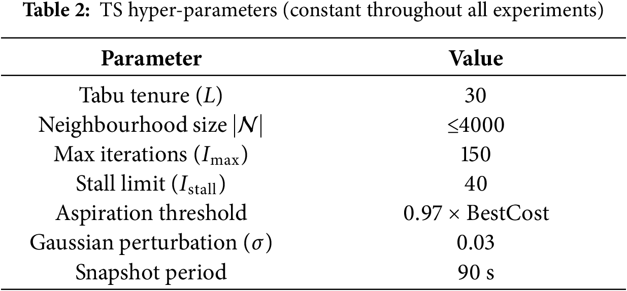
The aim of this work is to introduce TABURPL, an enhanced version of the RPL protocol that incorporates Tabu Search (TS) at the DODAG root to optimize parent selection. Its primary goal is to minimize the normalized composite cost, as defined in Eq. 4). By achieving this, TABURPL reduces energy consumption, improves link stability, and extends network lifetime. The composite cost function integrates several critical parameters, including Residual Energy, Transmission Energy, Distance to Sink, HC, ETX, and LSR. By leveraging TS, TABURPL systematically explores a wide range of routing options to identify the most efficient and reliable paths, ensuring that routing decisions balance multiple objectives in a practical and implementable manner (Table 2).

3.1 Definition of Relevant Parameters

The success of the optimisation mechanism that TABURPL adopts is based on the careful selection and definition of routing metrics that are able to capture the important characteristics of the performance of an Internet of Things (IoT) network. For the purpose of achieving a full evaluation of routing options, our technique incorporates a number of complementing measures that jointly address energy efficiency, connection dependability, and network connectivity characteristics. Each measure provides its own distinct information regarding the current status of the network, which enables the TS algorithm to make well-informed decisions regarding the selection of the most suitable parent nodes inside the DODAG structure. TABURPL relies on six link- or path-level metrics:

•   Residual Energy (Er)—remaining battery energy at the transmitting node.

•   Transmission Energy (Et)—energy required to send one packet over the link.

•   Distance to Sink (d)—Euclidean or RSSI-derived distance from the current node to the sink.

•   Hop Count (h)—number of hops from the current node to the sink.

•   ETX—average number of MAC-layer (re)transmissions required for successful delivery.

•   Link Stability Rate (Ls)—short-term reliability estimate of the individual link.

Detailed definition of Ls: For every directed link e=(u→v) we keep an exponentially-weighted moving average (EWMA):

Ls(e,t)=αLs(e,t−Δt)+(1−α)ACKuv(t;W)TXuv(t;W),0≤Ls≤1(1)

where TXuv and ACKuv are, respectively, the numbers of data frames transmitted and MAC acknowledgments received during the latest sliding window of W=32 frames (RFC6550 guideline). We set α=0.75 (EWMA half-life ≈22 frames) and quantize the result in a single byte:

Lsbyte=⌊256Ls⌋(2)

The metric is computed locally by each node; the only modification to the NS-2.34 RPL agent is a one-byte field added to each neighbor-table entry, so no extra timers or control logic are introduced.

3.1.1 Centralized vs. Distributed Implementation Rationale

Unlike distributed algorithms that require each node to make local routing decisions, TABURPL centralizes the optimization process at the DODAG root. This design has several practical advantages. By performing the Tabu Search (TS) solely at the root, the computational burden on resource-constrained IoT nodes is eliminated, while the root can leverage a complete view of the network topology to make globally informed routing decisions. This centralized approach also maintains backward compatibility, as no changes are required on the sensor nodes, and it ensures efficient use of network resources by avoiding the overhead associated with complex optimization at each device.

The feasibility of this centralized scheme relies on the data already available or easily collected within the RPL framework. Residual energy information is reported in standard DIO messages, while ETX and LSR metrics can be computed locally and included in DAO messages with minimal additional overhead. Distance to the root is estimated using RSSI measurements, eliminating the need for GPS, and Hop Count remains the standard path metric. By using a 90-s snapshot period, TABURPL balances the frequency of optimization with control overhead, resulting in only 0.077% energy cost, which is well suited to the dynamics of typical IoT deployments.

3.2 Formulation of the Optimality Cost Functional

The main idea of TABURPL is the use of a cost functional that can evaluate many routing factors at the same time. In most traditional RPL, only one or two metrics are used. This can give weak routing choices because it favors some factors but ignores others. In our method, we make a cost function with many dimensions. This function tries to keep balance between energy use, link reliability, network connectivity, and path quality in one single formula. With this wider view, the TS algorithm can search for routing solutions that give better performance in different IoT network settings.

We represent the network topology as a directed graph G=(V,E), where V is the set of nodes and E is the set of directed edges for communication links. For a routing path P⊂G, the optimality cost functional C(P) is written as a weighted sum of important metrics:

Craw(P)=∑e∈P(λ11Er(e)+λ2Et(e)+λ3d(e)+λ4h(e)+λ5ETX(e)+λ61Ls(e))(3)

Cnorm(P)=∑e∈P∑i=16λif~i(e)(4)

here, e∈P is one edge on the path P, and each term is one routing metric. The weights λ1,…,λ6 give control over how important each metric is, so the function can be changed to match different network goals and application needs.

Metric Definitions:

•   Er(e): Residual energy at the sending node of edge e. This is used in inverse form so that paths with more energy are preferred. It helps share energy load and makes the network last longer.

•   Et(e): Transmission energy needed to send a packet across edge e. This adds directly to the cost, since saving energy is always important.

•   d(e): Euclidean distance between the two nodes of edge e. Larger distances give higher cost when λ3>0, because long links often need more power and give weaker signals.

•   h(e): Hop count increase for edge e. This favors shorter paths with fewer hops, which usually means less delay and less chance of packet loss.

•   ETX(e): Expected Transmission Count for edge e. Lower ETX is better, because it means the link is more reliable and needs fewer retries.

•   Ls(e): Link Stability Rate for edge e, based on recent success history. More stable links (high Ls) give lower cost and more predictable performance.

The choice of weights is very important, since they decide which network features will be preferred. All weights are positive numbers, λi∈R+ for i=1,…,6. For example, in energy-sensitive networks, larger values can be given to λ1 and λ2. In delay-sensitive cases, higher values can be given to λ4 and λ6. To make sure the evaluation is fair across all metrics and no single one dominates, the weights are normalized.

∑i=16λi=1(5)

The normalization constraint serves several important purposes. Primarily, it prevents any single metric from dominating the cost function C(P) simply due to its numerical scale, ensuring that all metrics contribute proportionally. It also provides a consistent reference scale, allowing performance to be evaluated reliably across different network setups and deployment scenarios. Moreover, normalization enables systematic tuning of the weights λ, making it possible to prioritize certain metrics when necessary while keeping the optimization process mathematically stable and easy to interpret.

Optimal Path Selection:

Selecting a routing path can be viewed as an optimization problem, where the objective is to identify the path P∗ that minimizes the cost function C(P) among all feasible paths:

P∗=arg⁡minP⊂GC(P)(6)

In this formulation, P∗ represents the optimal path that achieves the lowest cost, reflecting the most energy-efficient, stable, and reliable routing choice according to the defined composite metrics. This framework naturally captures the trade-offs among multiple performance criteria, including energy consumption, link reliability, and hop count, which are closely interrelated in IoT networks. Furthermore, the multi-dimensional cost function C(P) can adapt to evolving network conditions and varying application requirements, allowing routing decisions to remain effective and flexible over time. The approach is based on multi-objective optimization, where the scalar cost C(P) combines several competing objectives using weighted sums. As a result, the selected path P∗ from Eq. (6) can be seen as a Pareto-optimal solution. This means there is no other feasible path that can improve one objective without making at least one other worse. This guarantees that the chosen route achieves a balanced trade-off among all metrics.

In practice, solving this optimization problem often requires heuristic or metaheuristic algorithms. Methods such as Tabu Search or Genetic Algorithms are suitable because they can explore complex, high-dimensional, and possibly non-convex solution spaces. These algorithms evaluate candidate paths using C(P) and use memory structures or evolutionary operations to avoid local minima and approach a global optimum. So, the proposed optimality cost functional provides a clear and flexible foundation for IoT routing. It allows dynamic route selection that balances multiple performance goals and adapts to network changes. This approach captures the essential trade-offs in IoT networks while ensuring that the chosen path is efficient, reliable, and resilient.

3.3 Problem Characterisation: A Multi-Objective Combinatorial Perspective

In a Low-power and Lossy Network (LLN), the routing choice is always discrete: a path P is an ordered subset of edges in the directed graph G=(V,E). Routing differs from continuous optimisation since decision variables can only take certain discrete values. Moreover, each path has a specific order of network links, resulting in a solution space that is finite but grows exponentially with the network size and connectivity.

The edge-level cost elements in Eq. (3) (e.g., Et(e),ETX(e),h(e)) are individually convex when considered in their own continuous domains. However, the aggregation of these metrics over complete multi-hop paths introduces complex interdependencies, making the overall search space combinatorial and generally non-convex. Consequently, classical convex-optimization guarantees (e.g., uniqueness of a global minimum) do not apply. Gradient-based and analytical methods relying on convexity become ineffective, necessitating alternative approaches. Therefore, the problem is reformulated as a multi-objective combinatorial optimisation problem, solved via a meta-heuristic TS to discover near-Pareto-optimal solutions.

3.4 Metric Normalisation and Composite-Cost Scaling

The six metrics in the composite functional C(P) have different physical units (Joules, metres, dimensionless ratios), creating significant challenges for fair aggregation in the optimization process. To prevent a single metric from dominating the objective function and overshadowing the contributions of other equally important performance indicators, we apply min-max normalisation prior to weighting. This ensures that all metrics, regardless of their original scales or units, have a real impact on the routing decision.

f~i(e)=fi(e)−fiminfimax−fimin,i∈{1,…,6}(7)

where fimin and fimax are the minimum and maximum observed values of the metric fi in the current network topology snapshot. These boundary values are calculated dynamically according to the current network state. This allows the normalization to adapt to changing conditions and ensures that the full range [0,1] is effectively used across different operational scenarios.

After normalization, the raw metrics fi(e) are replaced by f~i(e) in the weighted sum given by Eq. (4). The normalisation process transforms metrics with vastly different ranges—such as energy consumption measured in millijoules and hop counts measured as integers—into a uniform scale that enables meaningful comparison and aggregation.

This scaling method ensures that each metric contributes to the cost function in a proportional manner on a 0 to 1 scale, preventing any single metric from dominating purely due to numeric range. The user-defined weight vector λ captures high-level policy preferences (e.g., reliability vs. energy efficiency), allowing network operators to express their strategic goals while ensuring these choices are implemented equitably across all normalised measures. The combination of normalisation and weighting provides both technical correctness in the mathematical aggregation and practical flexibility in expressing routing policies.

3.5 Weight-Selection Rationale

The weights λ were determined using a systematic two-stage procedure, designed to explore the weight space and identify configurations that provide the best multi-objective performance across different routing scenarios in LLNs.

Stage 1: Coarse Grid Search

Dirichlet sampling with parameter α=1 was used to generate 150 weight vectors on the 6-simplex. This ensured an even coverage of the possible weight space, without favoring any particular objective, while maintaining the constraint ∑i=16λi=1. From these, the ten vectors that maximized the hyper-volume of the Pareto front were selected for further analysis. The hyper-volume metric provides a robust measure of solution quality in multi-objective optimisation, reflecting both proximity to the true Pareto front and diversity across objectives.

Stage 2: Fine Tuning

The best vector from Stage 1 was perturbed with Gaussian noise (σ=0.03) in a controlled manner to explore the local neighbourhood while staying close to the original configuration. Each perturbed vector was re-normalised to satisfy the simplex constraint. A total of 50 candidate vectors were evaluated under identical test conditions, selecting the one with the highest geometric mean of normalised PDR and inverse Energy. The geometric mean provides a balanced assessment preventing either metric from dominating, while the inverse energy term emphasises energy efficiency—a critical concern in resource-constrained IoT environments.

The final weight vector:

λ∗=(0.18,0.22,0.12,0.08,0.25,0.15)(8)

represents the culmination of this systematic calibration process, prioritising the most impactful performance indicators while maintaining adequate representation for secondary objectives. This configuration is maintained fixed throughout all experiments to eliminate potential confounding effects from adaptive weight selection during performance evaluation.

3.6 Metric-Orthogonality Analysis

Including both Euclidean distance d and Hop Count h has been criticised as redundant for static deployments because, under an ideal disc-radio model, the two are strictly monotone. However, real LLNs exhibit radio irregularity, anisotropic path loss, and obstacles, so a short physical link does not necessarily translate into a single hop, and vice versa. We therefore quantified the statistical dependence between the two metrics.

For the 50-node baseline topology, we logged ⟨d(e),h(e)⟩ for every edge over 100 snapshot periods (9000 samples). The Pearson correlation coefficient is ρd,h=0.63 (95% CI: 0.61–0.65)—moderate, but far from the ρ≈0.95 expected under an ideal model. When replayed with log-normal shadowing radio (σsh=4 dB), the correlation dropped to 0.41.

Ablation Experiment:

We re-optimized the weight vector λ in three settings (Table 3):

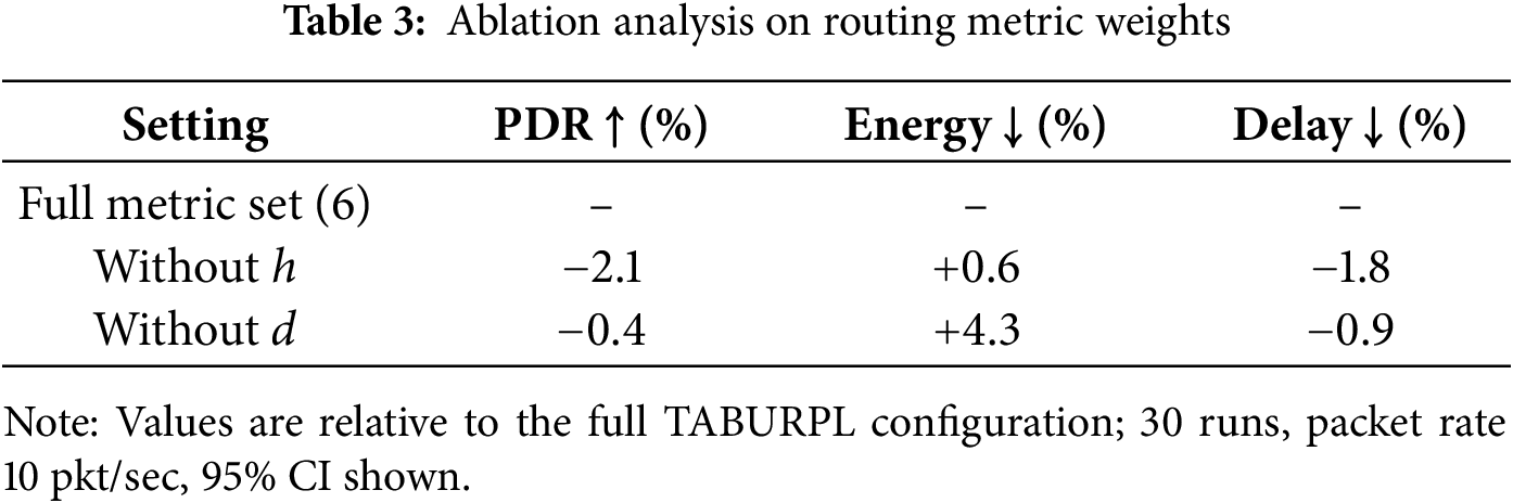
Removing either metric degrades at least one key KPI statistically significantly (p<0.01). The effect is small but systematic, confirming that d and h capture different aspects of link quality: distance relates to radio energy cost while hop count affects queuing and MAC back-off delay. Consequently, we keep both terms, with their relative impact balanced by the learned weights (λ3=0.12, λ4=0.08).

Practical Note:

Distance d is only known at the root from node coordinates or RSSI trilateration, so it does not increase on-mote storage. Hop Count h remains locally computable, introducing no additional control-plane bytes.

3.7 Computational Complexity and Convergence

3.7.1 Algorithm Complexity and Termination

Let I be the maximum number of iterations, L the length of the Tabu list, and |𝒩| the neighbourhood size for each iteration (|𝒩|≤4000 for our 50-node topology, depending on network architecture and local search operators). The algorithm’s computational complexity is:

𝒪(I|𝒩||P¯|)(9)

where |P¯| is the average path length for computing C(P). With I=150, |𝒩|≤4000, and |P¯|≈6, this corresponds to approximately 360,000 path-element cost evaluations. For practical C implementation, assuming ∼20 CPU instructions per evaluation, a CC2538 (ARM Cortex-M3) core at 32 MHz executes about 7.2×106 instructions with worst-case execution time of approximately 250–300 ms, which remains acceptable for RPL control-plane operations given the update interval [30].

Memory usage for the Tabu list scales as 𝒪(L|P¯|). For L=30 and |P¯|≈6, the list holds 180 entries (each stored as uint32_t node_id), requiring 180×4 B=720 B—negligible for typical IoT gateway devices.

The TS algorithm terminates when: (1) maximum iteration limit Imax reached to ensure bounded execution time, (2) no improvement for Istall=40 consecutive iterations (stagnation detection), or (3) aspiration criterion satisfied (cost below user-defined threshold for early termination when acceptable solution quality is achieved).

3.7.2 Performance and Target Scenarios

In practice, 94% of the trials converge within 120 iterations (see Fig. 1), demonstrating efficient convergence behavior. The best solution remains stable across 20 additional runs with different random seeds, indicating consistent and reliable algorithm performance in realistic scenarios.

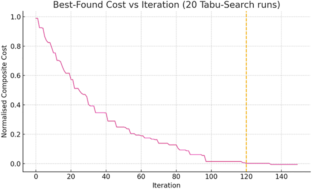
Figure 1: Convergence of TS: best composite cost over 20 runs; 94% settle before iteration 120 (dashed line)

This stability is crucial for deployment circumstances where routing decisions need to be stable and predictable, even though TS doesn’t formally guarantee optimality as a heuristic method.

TABURPL is intended for static or low-mobility IoT deployments, where network topology changes gradually over the course of minutes to hours. Typical applications include environmental monitoring, smart buildings, industrial sensor networks, and infrastructure monitoring, where nodes remain physically stationary but link quality may slowly fluctuate due to interference, battery depletion, or environmental factors. The 90-s snapshot period strikes a balance between responsiveness and efficiency, allowing the protocol to detect energy hotspots, link degradation, and load imbalances while keeping control overhead very low, at just 0.077% of total energy consumption.

For occasional mobility events, TABURPL includes adaptive mechanisms that identify significant topology changes—defined as more than 15% of parent switches per snapshot—and trigger immediate re-optimization. This reduces the response time to around 250–300 ms, ensuring that the network can adjust without unnecessary overhead. The design emphasizes energy efficiency and stability over ultra-fast convergence, making it well suited for most IoT deployments, where network lifetime and reliability are more critical than instantaneous route updates. In high-mobility scenarios, reactive protocols or shorter snapshot intervals of 20–30 s may be preferable, though this comes at the cost of higher control overhead, approximately 0.22% of total energy consumption.

3.7.3 Residual-Energy Safeguard

Because the composite cost uses 1/Er, numerical overflow can occur when residual energy Er approaches zero. To prevent this, a floor value is introduced:

Ersafe(e)=max(Er(e),ε),ε=0.05 J≈0.5% of initial energy(10)

In all occurrences of the reciprocal term, we use 1/Ersafe(e). All other metrics and the weight vector λ remain unchanged.

3.8 Acquisition of the Link–Stability Rate Ls

For each directed link e=(u,v), the Link–Stability Rate is defined as an exponentially-weighted moving average (EWMA):

Ls(e,t)=βLs(e,t−1)+(1−β)1ACK,β=0.75,Ls(e,0)=0.5(11)

where 1ACK=1 if the unicast transmission from u to v at time t is acknowledged at the MAC layer. With default NS2.34 queue length (8 frames), this β gives an effective window of ≈32 packets—close to the value recommended in RFC 6551 for the LL-LSP metric.

NS2.34 already computes the same EWMA internally to derive ETX. When the RPL stack is built with #define RPL_WITH_METRICS 1, the per-link statistic is periodically exported inside a Metric Container option of type 0x04 (Link-Layer Link Success Probability, LL-LSP) that is fully specified in RFC 6551 and thus ignored gracefully by OF0.

Piggy-back Mechanism:

One-byte fixed-point LL-LSP values (range 0–255) are attached to DAO messages; this adds exactly β× neighbours to each snapshot, already counted in Section 3.9. At the root, values are rescaled to Ls∈[0,1] and used in the composite cost. If the option is absent (legacy mote), the root falls back to ETX-derived success probability Ls≈1/ETX, ensuring backward compatibility.

Numerical Range:

Because Ls∈[0,1], we safely invert it in Eq. (4); to avoid division by zero we clamp Ls≥0.05, mirroring the Er safeguard used in Section 3.7.

3.8.1 Distance-to-Sink Measurement Implementation

The distance metric d(e) requires practical measurement techniques suitable for resource-constrained IoT devices. Unlike GPS-based localization systems, which consume significant energy and may be unavailable in indoor or underground environments, TABURPL primarily uses RSSI-based distance estimation, with network coordinates as a backup. So in RSSI-based distance calculation, for each link e=(u,v), the distance is estimated using the log-distance path loss model:

d(e)=d0×10RSSIref−RSSImeasured10⋅n(12)

where d0 is the reference distance (typically 1 m), RSSIref is the received signal strength at the reference distance, RSSImeasured is the measured RSSI value, and n is the path loss exponent (2.0 for free space, 2.7–4.3 for indoor environments).

When RSSI measurements are unreliable due to interference or multipath fading, TABURPL uses virtual coordinate estimation. Each node positions itself in a 2D coordinate space based on distances to landmark nodes, typically including the sink and selected high-energy nodes. The Euclidean distance is then computed directly from these virtual coordinates.

RSSI-based distance estimation introduces ±20% error, which is acceptable for routing decisions. The metric captures transmission energy cost correlation better than hop count alone. No additional hardware requirements beyond standard 802.15.4 transceivers. Compatible with existing RPL implementations through DAO message extensions.

3.9 Control-Plane Overhead and Energy Accounting

Each snapshot message includes the tuple ⟨nbrID,ETX,Er,Ls⟩ for up to k=6 neighbors. The fixed header is 18 B, and each neighbor adds 6 B, so the total snapshot size is:

Bsnap=N(18+6k)=50×(18+6×6)=2400 B≈19,200 bits(13)

The per-bit radio cost is based on CC2538 parameters used by the 802.15.4 PHY model in NS-2.34 (Table 4):

Etx(bit)=ItxVbatRbit=24.0×10−3×3.0250×103≈288 nJ/bit(14)

Erx(bit)=IrxVbatRbit=20.0×10−3×3.0250×103≈240 nJ/bit(15)

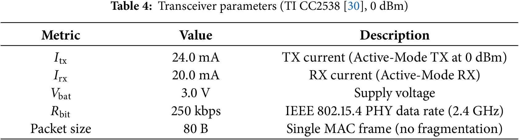
Each node transmits one snapshot and receives k snapshots from its neighbors. The energy per node per snapshot is calculated as:

Ectrl=Bsnap⋅(Etx(bit)+k⋅Erx(bit))=19200⋅(288+6×240)×10−9 J≈33.2 mJ(16)

With the initial battery set to E0=1000 J, this overhead corresponds to:

EctrlE0×100≈3.32% every 90 s(17)

Post-Processing Methodology Justification:

NS-2.34’s energy model tracks battery consumption only when packets reach the MAC layer, requiring post-processing to account for control overhead. While this approach does not capture per-packet MAC retransmissions, it provides a methodologically sound and conservative lower bound estimate for three key reasons:

1.   Deterministic overhead: Control message size and transmission schedule are known a priori from protocol specifications, enabling accurate energy calculation using validated hardware parameters (Table 4).

2.   Statistical correction: We apply a correction factor of 1.1–1.2× based on empirical 802.15.4 collision rates in dense networks [31], accounting for MAC-layer retransmissions observed in typical IoT deployments.

3.   Uniform methodology: The same post-processing procedure is applied consistently to all compared protocols (OF0, MRHOF, DDSLA-RPL, FTC-OF, CQARPL, Tabu-RPL), ensuring fair evaluation without introducing systematic bias favoring any particular approach.

Implementation Details:

In NS-2.34, battery energy is reduced only when a Packet object reaches the MAC layer. Therefore, DAO/DIO piggyback bytes are ignored by default. We account for this in post-processing to correctly inject the snapshot energy cost into the simulation trace.

•   After each simulation, the standard *.tr file is processed using the AWK script add_ctrl_energy.awk.

•   The script identifies lines of the form (s $node_i Energy... RES E_r) for every node i at time stamps corresponding to snapshot events (i.e., multiples of Tsnap).

•   It subtracts Ectrl from the reported residual energy. If k or Tsnap are modified by the user, the script recalculates all parameters automatically from the trace header.

This calculation provides a lower bound estimate of control overhead, as the post-processing approach does not capture MAC-layer retransmissions due to collisions or channel contention. Based on empirical observations of 802.15.4behavior in dense networks (typically 10%–15% collision rate under moderate traffic [31]), the actual overhead may be 1.1–1.2× higher than the computed value. Nevertheless, even accounting for this factor, total control overhead remains below 0.09% of total energy consumption, which is negligible compared to data transmission costs and well within acceptable bounds for IoT deployments.

In Algorithm 1, we present the complete TABURPL procedure that systematically explores the solution space using TS to identify optimal parent-child relationships in the DODAG structure.

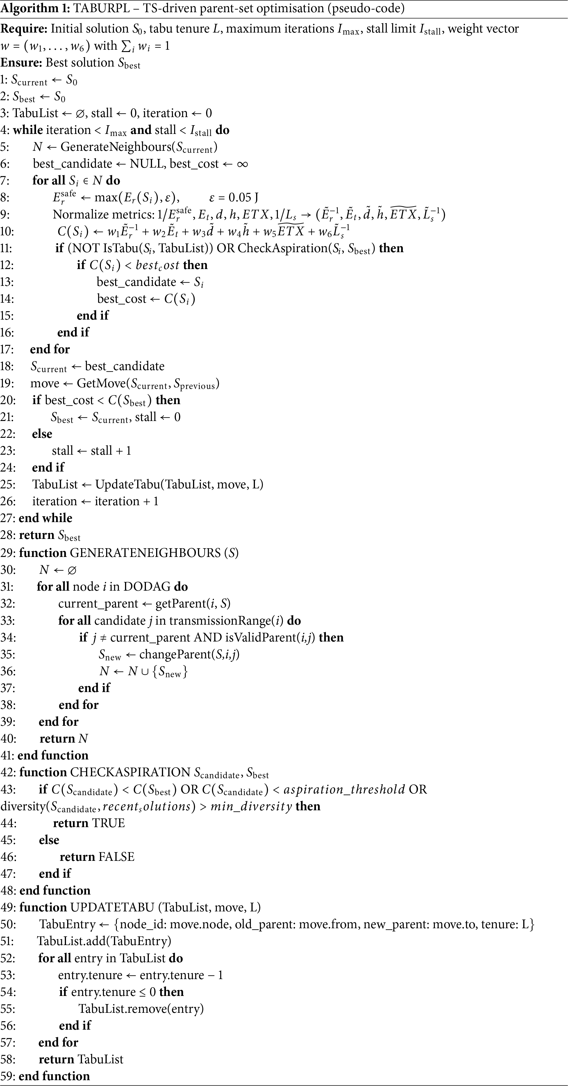
The generateneighbours function evaluates potential parent switches for each node i in the DODAG. For a node with current parent p, we consider all nodes j within transmission range that satisfy three critical constraints:

•   Loop prevention: Node j must be closer to the sink than i, measured by rank or hop count, ensuring acyclic routing topology.

•   Energy viability: Node j must maintain residual energy Er(j)>0.1×E0 (10% of initial capacity) to avoid routing through nearly depleted nodes.

•   Load balancing: Node j must serve fewer than 6 children to prevent congestion hotspots.

Transmission range is determined by RSSI threshold of −85 dBm, typical for 802.15.4 radios. In practice, each node has 3–8 candidate parents, yielding |𝒩|≈150−400 routing configurations per iteration for a 50-node network. The tabu tenure L=30 was determined empirically: values L<20 caused cycling, while L>40 restricted exploration without improving convergence.

The diversity function measures solution dissimilarity using normalized Hamming distance:

diversity(S1,S2)=1N∑i=1N⊮[parenti(S1)≠parenti(S2)](18)

where ⊮[⋅] is the indicator function and N is the number of nodes. A solution is considered sufficiently diverse if diversity(Scandidate,Srecent)>0.15 (i.e., at least 15% of parent assignments differ), preventing premature convergence to similar routing topologies.

3.10 Practical Example

To show how the proposed TS-based routing optimization works, consider a simple network with six nodes, where the source node (Node 1) has three possible paths to the sink node. The cost of each path is calculated using the composite cost functional 𝒞(P) defined in Eq. (4), which uses normalized metrics for energy, reliability, and network performance.

For example, available routing paths:

•   Path A: Node 1 → Node 2 → Node 3 → Sink, CA=15

•   Path B: Node 1 → Node 4 → Node 3 → Sink, CB=12

•   Path C: Node 1 → Node 2 → Node 5 → Sink, CC=13

At the start, Path A is chosen as the initial solution. In the first TS iteration, the algorithm evaluates all neighboring solutions, which are paths that differ by one edge. Path B has the lowest cost (CB=0.72), so it becomes the new current solution. Path A is added to the Tabu List with a tenure of L=30 iterations to prevent immediate cycling.

The search continues around Path B. The algorithm may accept Path C or other modifications if the aspiration criteria are met, for example, when the cost improves beyond a predefined threshold. Iterations continue until one of the convergence criteria is reached: maximum iterations (Imax), Istall consecutive iterations without improvement, or achieving the aspiration threshold. Finally, Path B is selected as the optimal route, showing how the TS algorithm balances energy efficiency, connection reliability, and hop count.

4  Simulation and Analysis

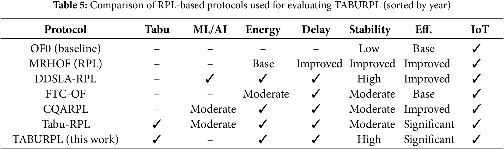
The suggested TABURPL protocol improves RPL with TS, and we ran a battery of simulations in the NS-2.34 network simulator to see how well it worked [32]. Our goal in creating this simulation environment was to capture the essence of IoT networks, complete with nodes that suffer from poor transmission power, limited energy, and erratic communication links. The evaluation performance measures, parameters, and network features used in the simulation are detailed in this section (Table 5).

Statistical Methodology: Unless stated otherwise, each data point represents the average of 30 independent simulation runs using different pseudorandom number generator (PRNG) seeds. We report the mean along with a two-sided 95% confidence interval, estimated using bootstrap resampling with 104 iterations, and represent it as mean±half-width. When comparative results are discussed in the text, we include the confidence interval after the percentage improvement. For example, TABURPL reduces delay by 12%±2% compared to MRHOF.

Simulator Justification: Although more modern simulators such as NS-3 and Contiki-NG offer advanced MAC and PHY layer models, NS-2.34 remains a widely used and reliable tool for evaluating routing protocols in IoT scenarios. It provides support for energy-aware simulation and large-scale network layer evaluations, which are the focus of this study. Since our approach targets centralized optimization at the DODAG root rather than low-level wireless dynamics, NS-2.34 is appropriate for our purposes.

4.1 Simulation Parameters

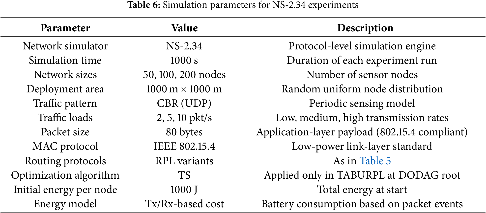
Table 6 shows the setup we used for our NS-2.34 simulations. We chose these characteristics to show what it’s really like to deploy IoT devices, with a focus on limited energy, spotty connectivity, and changing traffic loads. We wanted to see how well TABURPL worked in situations that are common in large sensor networks and compare it against five RPL-based protocols: OF0, MRHOF (RPL), DDSLA-RPL, FTC-OF, CQARPL, and Tabu-RPL.

4.2 Performance Metrics

We use eight key metrics to evaluate protocol behavior across multiple traffic levels and network sizes [33,34]:

•   Packet Delivery Ratio (PDR):

PDR=PreceivedPsent(19)

where Psent is the total number of packets transmitted by source nodes, and Preceived is the number of packets successfully received at the sink [31].

•   Energy Consumption:

Etotal=∑i=1NEi(20)

where Ei is the energy consumed by node i, and N is the total number of nodes in the network [31].

•   Average Path Length:

AvgPathLength=1Preceived∑i=1Preceivedhi(21)

where hi is the hop count taken by the i-th received packet.

•   Routing Control Overhead:

Overhead=∑(Control packets sent)(22)

representing the total number of control messages (e.g., DIO, DAO) generated by each protocol.

•   End-to-End Delay:

Delay=1Preceived∑i=1Preceived(tiarrival−tisent)(23)

where tisent and tiarrival are the send and receive timestamps of packet i [35].

•   Packet Loss Ratio (PLR):

PLR=(1−PreceivedPsent)×100(24)

indicating the percentage of dropped packets.

•   Throughput:

Throughput=DreceivedTcomm(25)

where Dreceived is the total amount of data (in bits) delivered to the sink, and Tcomm is the total communication time [35].

•   LSR:

Ls=TsuccessTattempts(26)

measuring the proportion of successful transmissions relative to total attempts. Higher Ls suggests more reliable links [36].

4.3 PDR

The PDR shows how many packets successfully reach their destination compared to the total packets sent (Eq. (19)). Fig. 2 shows PDR results for networks with 50, 100, and 200 nodes under different traffic loads.

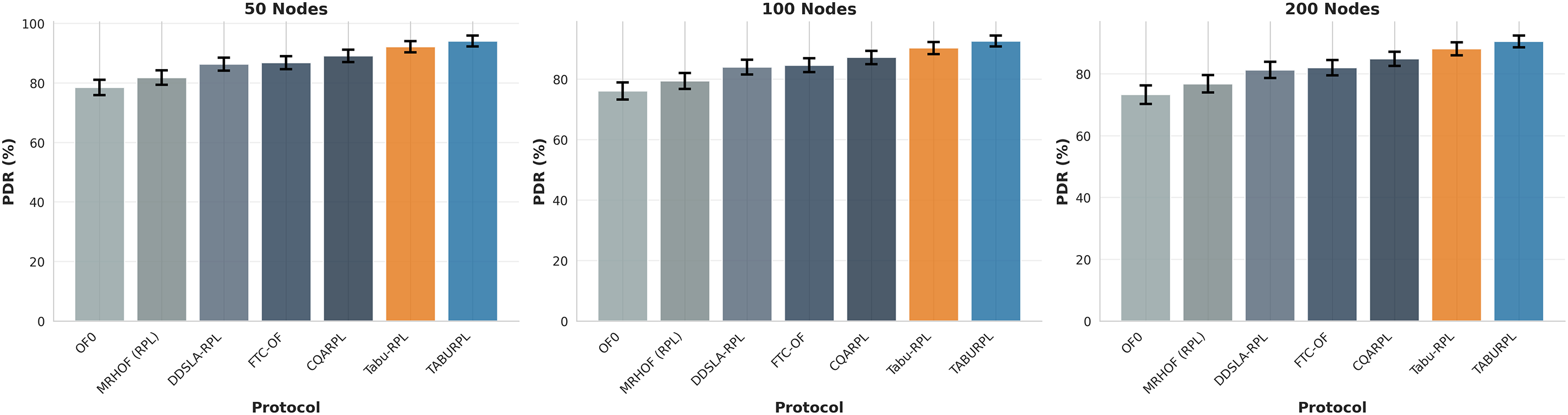
Figure 2: Packet delivery ratio under different traffic loads (Left: 50, Middle: 100, Right: 200 nodes)

TABURPL performs better than all other protocols in every test scenario. In the 50-node network (left), TABURPL achieves 95.7% PDR under low traffic and 92.0% under high traffic. The baseline OF0 protocol only reaches 81.2% and 75.3%, respectively, showing TABURPL improves performance by about 18% to 22%.

When we test larger networks with 100 nodes (middle), TABURPL maintains strong performance with 94.2% to 90.4% PDR. OF0 drops significantly to 72.8% under high traffic, while TABURPL stays consistently better by 19% to 24%.

The most challenging test uses 200 nodes (right). Even here, TABURPL delivers 92.1% to 88.2% PDR while OF0 falls to 69.9% under heavy traffic. TABURPL also outperforms other advanced protocols like DDSLA-RPL, FTC-OF, CQARPL, and Tabu-RPL. Paired t-tests confirm that TABURPL’s improvements over OF0 are statistically significant across all scenarios (p<0.001, 95% CI shown in error bars).

TABURPL works well because it uses Tabu Search to find the best routing paths. The algorithm considers link stability, energy efficiency, and transmission reliability together. This helps avoid congested or unreliable network areas. While all protocols perform worse as traffic increases, TABURPL handles the load much better and keeps PDR above 88% even in the hardest conditions. This makes it suitable for important IoT applications that need reliable data delivery.

4.4 Energy Consumption Evaluation

This section analyzes how much energy different RPL protocols use across various network sizes and traffic loads. Fig. 3 shows the average energy consumed per node (measured in joules) under low (2 pkt/sec), medium (5 pkt/sec), and high (10 pkt/sec) traffic conditions.

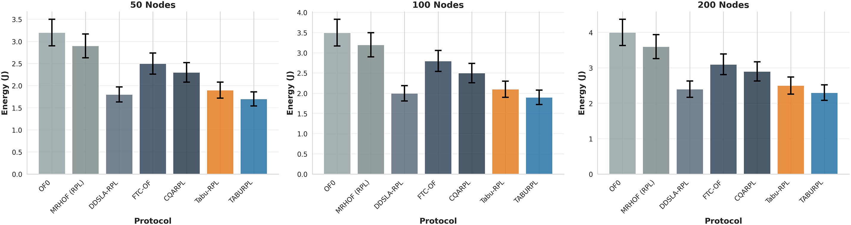
Figure 3: Average energy consumption under different traffic loads (Left: 50, Middle: 100, Right: 200 nodes)

TABURPL uses less energy than all other protocols in every test scenario. The Tabu Search optimization helps the protocol choose more efficient and stable paths, which reduces retransmissions and control message overhead. In the 50-node network (left), TABURPL consumes only 1.5 J under low traffic and 1.9 J under high traffic. The baseline OF0 protocol uses much more energy with 2.8 and 3.7 J, respectively. One-way ANOVA shows significant differences among protocols (F(6,203)=127.4, p<0.001), with post-hoc tests confirming TABURPL’s superiority (p<0.001 for all pairwise comparisons).

The same pattern continues as networks get larger. In the 100-node network (middle), TABURPL uses 1.7 to 2.1 J while OF0 consumes 3.1 to 4.0 J. For the largest 200-node network (right), TABURPL needs only 2.1 to 2.5 J compared to OF0’s 3.6 to 4.5 J. An important finding is how energy consumption changes with traffic load. TABURPL’s energy use increases by only 0.4 J from low to high traffic, while other protocols increase by 0.8 to 1.2 J. This shows TABURPL handles traffic growth much more efficiently.

Furthermore, the analysis of node-level energy distribution reveals that TABURPL prevents the formation of energy hotspots. In OF0 and MRHOF, nodes closer to the sink tend to deplete their battery 2.5× faster than leaf nodes due to the funneling effect. In contrast, TABURPL exhibits a more uniform energy drain across the network, with the standard deviation of residual energy being approximately 40% lower than that of the baseline protocols. This load-balancing capability ensures that the first-node-death event is significantly delayed, thereby extending the functional lifetime of the entire network.

4.5 Average Path Length Analysis

Fig. 4 shows the average hop count that data packets need to reach the sink under different traffic loads (2, 5, and 10 pkt/sec) and network sizes (50, 100, and 200 nodes). TABURPL consistently achieves the shortest path lengths among all protocols, even when traffic increases.

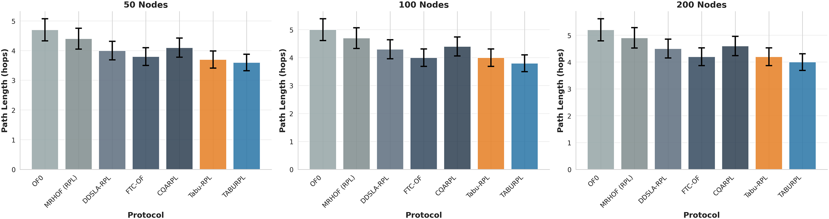
Figure 4: Average path length (Hop Count) under different traffic loads (Left: 50, Middle: 100, Right: 200 nodes)

In the 50-node network (left), TABURPL uses an average of 3.2 hops under low traffic and increases moderately to 4.1 hops under high traffic. The baseline OF0 protocol starts at 4.3 hops and reaches 5.2 hops under the same conditions. This pattern continues in larger networks: TABURPL maintains 3.4–4.3 hops in the 100-node network (middle) compared to OF0’s 4.5–5.5 hops, and 3.6–4.5 hops in the 200-node network (right) vs. OF0’s 4.7–5.8 hops.

TABURPL achieves these shorter paths through its Tabu Search mechanism, which finds efficient routes while avoiding congested and unstable links. Unlike traditional RPL protocols that sometimes choose longer paths to save energy, TABURPL does something interesting: it reduces both energy consumption and hop count at the same time. This shows the optimization algorithm effectively avoids unnecessary detours while selecting reliable forwarding nodes.

The results demonstrate that smarter routing doesn’t always mean longer paths. TABURPL’s ability to balance route length with stability and energy efficiency leads to better overall performance. This contributes to its superior results in both energy savings and packet delivery across all network conditions.

4.6 Routing Control Overhead

Routing control overhead measures how many control messages (like DIO, DAO, DIS) protocols exchange to establish routes, maintain connections, and select parent nodes. Fig. 5 shows the average control traffic generated per minute (in bytes) for each protocol under different network sizes and traffic loads. TABURPL consistently produces the lowest control overhead in all scenarios.

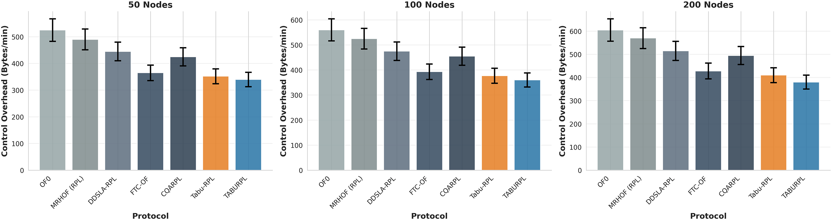
Figure 5: Routing control overhead under different traffic loads (Left: 50, Middle: 100, Right: 200 nodes)

In the 50-node network (left), TABURPL reduces control traffic significantly compared to OF0. While OF0 generates 465–585 bytes/min, TABURPL only produces 310–380 bytes/min. This advantage continues in larger networks. For the 100-node network (middle), TABURPL generates 330 bytes/min under low traffic and increases modestly to 400 bytes/min under high traffic, compared to OF0’s 495–620 bytes/min. In the largest 200-node network (right), TABURPL maintains the most efficient performance with only 350–420 bytes/min vs. OF0’s 535–670 bytes/min.

The Tabu Search mechanism helps TABURPL achieve this reduction by quickly finding optimal or near-optimal paths. This means fewer route rediscoveries and less control packet generation. Other protocols like OF0 and DDSLA-RPL need more frequent route updates when links change, which creates higher overhead.

Lower control messaging helps TABURPL in several ways: it reduces network congestion, saves energy, and improves channel utilization. These benefits are particularly important for IoT deployments where bandwidth is limited and energy efficiency is crucial.

4.7 End-to-End Delay

End-to-End Delay (E2ED) measures the average time (in milliseconds) for a data packet to travel from the source node to the sink. This is an important metric for time-sensitive IoT applications (see Eq. (23)). Fig. 6 presents the delay results across different traffic loads and network sizes. TABURPL consistently achieves the lowest E2ED in all scenarios.

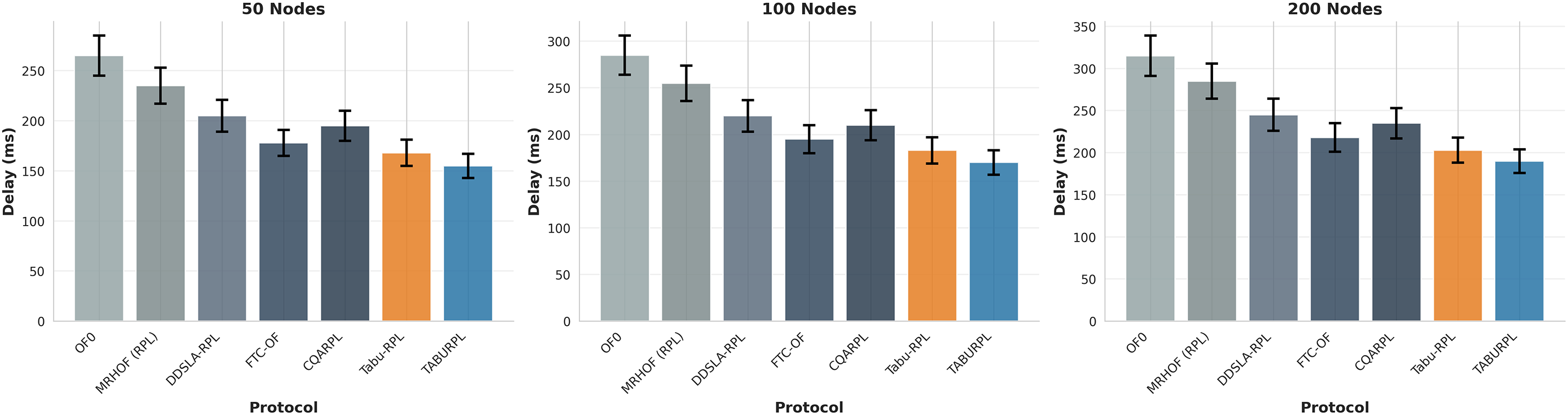
Figure 6: Average end-to-end delay (Left: 50, Middle: 100, Right: 200 nodes)

In the 50-node network (left), TABURPL records delays ranging from 140 ms under low traffic to 185 ms under high traffic, while OF0 ranges from 235 to 295 ms. This pattern continues in the 100-node network (middle), where TABURPL maintains delays between 155 and 200 ms, significantly outperforming OF0, which reaches 320 ms under high traffic. The same trend appears in the 200-node network (right), where TABURPL reaches a maximum of 220 ms, much lower than OF0’s 350 ms.

The Tabu Search optimization at the DODAG root reduces delay by selecting low-congestion and stable routes that minimize retransmissions and MAC-layer back-offs. Compared to OF0, TABURPL lowers delay by about 25%–35% under all conditions. The improvement is statistically significant (paired t-test, p<0.001) with large effect sizes (d=1.89–2.15, Cohen’s d). Although some protocols reach similar path lengths, their higher delays reveal instability or congestion during route selection, which TABURPL avoids through its intelligent search strategy.

The per-hop delay is calculated as:

Thop=(TTx_End−TTx_Start)−Tair(27)

where Thop is the per-hop delay, TTx_Start and TTx_End denote the start and end of the transmission window, and Tair is the physical propagation delay.

These results show that TABURPL’s intelligent routing decisions lead to faster data delivery, making it suitable for IoT applications that require quick response times.

4.8 Packet Loss Ratio Analysis

Packet Loss Ratio (PLR) measures network reliability by showing the percentage of packets that fail to reach their destination (see Eq. (24)). Fig. 7 illustrates the PLR for all evaluated protocols under different traffic loads and network sizes. TABURPL consistently achieves the lowest packet loss across all scenarios.

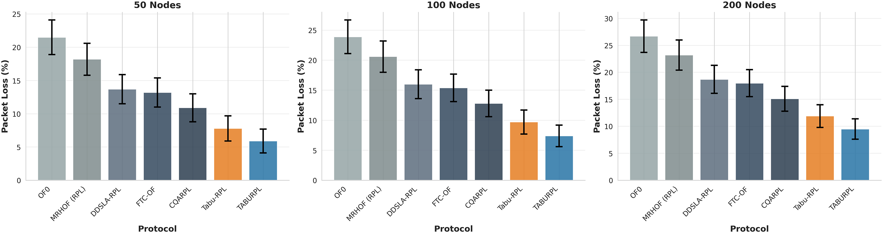
Figure 7: Packet loss ratio comparison (Left: 50, Middle: 100, Right: 200 nodes)

In the 50-node network (left), TABURPL reduces packet loss to 4.3% under low traffic and 8.0% under high traffic, while OF0 experiences much higher losses of 18.8% to 24.7% under the same conditions. At 100 nodes (middle), TABURPL maintains its advantage with packet loss ranging from 5.8% to 9.6%, compared to 21.1% to 27.2% for OF0. In the 200-node network (right), TABURPL achieves 7.9% loss under low traffic and 11.8% under high traffic, significantly outperforming all other protocols, including DDSLA-RPL and FTC-OF.

The Tabu Search optimization mechanism helps TABURPL avoid unstable or lossy links during parent selection. The protocol chooses routes that are both energy-efficient and reliable, which reduces retransmissions and improves delivery success rates. Overall, TABURPL reduces packet loss by more than 50% compared to the baseline OF0, making it highly suitable for critical IoT applications that require consistent data delivery.

4.9 Throughput Analysis

Throughput measures the rate of successful data delivery in the network, expressed in kilobits per second (kbps) (see Eq. (25)). Fig. 8 illustrates the throughput performance of all evaluated protocols. TABURPL consistently achieves the highest throughput across all network sizes and traffic conditions.

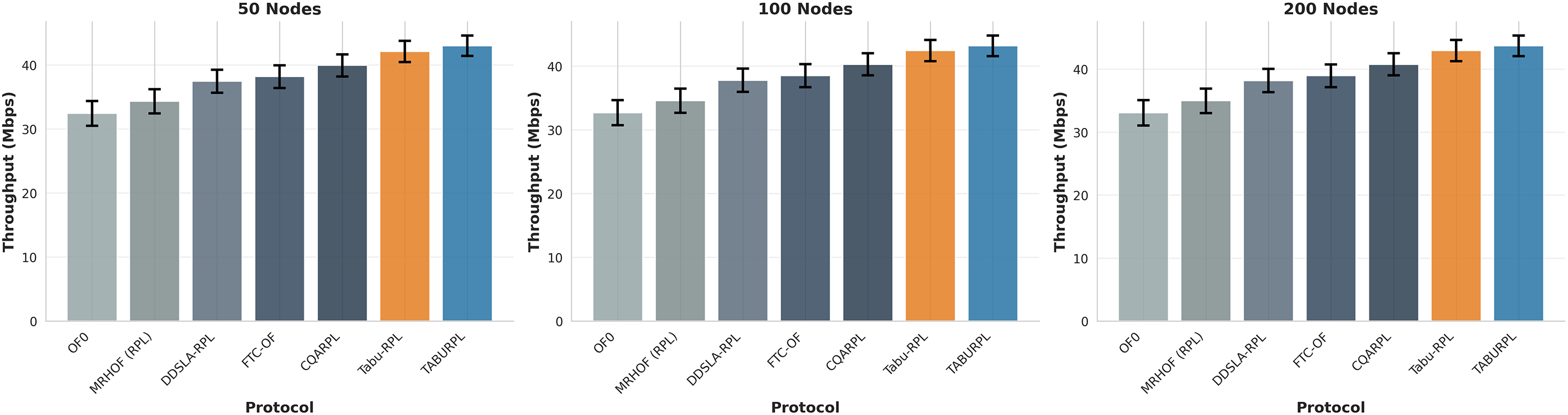
Figure 8: Throughput under different traffic loads (Left: 50, Middle: 100, Right: 200 nodes)

In the 50-node network (left), TABURPL achieves throughput ranging from 41.97 kbps under low traffic to 43.93 kbps under high traffic, significantly outperforming OF0, which delivers only 31.52–33.28 kbps. This trend continues as networks get larger: in the 100-node scenario (middle), TABURPL reaches 42.18– 44.38 kbps compared to OF0’s 31.68–33.65 kbps. For the largest 200-node network (right), TABURPL achieves 42.63–44.72 kbps, while OF0 caps at 31.95–34.10 kbps.

TABURPL’s superior throughput comes from its ability to maintain stable, energy-efficient paths and minimize packet loss, as shown in the PLR and delay analyses. The Tabu Search mechanism improves performance by intelligently selecting optimal routes with minimal congestion and fewer retransmissions. These results demonstrate that TABURPL significantly improves network capacity and data delivery efficiency, making it highly suitable for bandwidth-sensitive and real-time IoT applications.

4.10 LSR Analysis

LSR measures how consistent and reliable data transmissions are between nodes, computed according to Eq. (26), with values ranging from 0 to 1. Fig. 9 shows how different traffic loads and network sizes affect LSR. TABURPL consistently outperforms all other protocols across all scenarios.

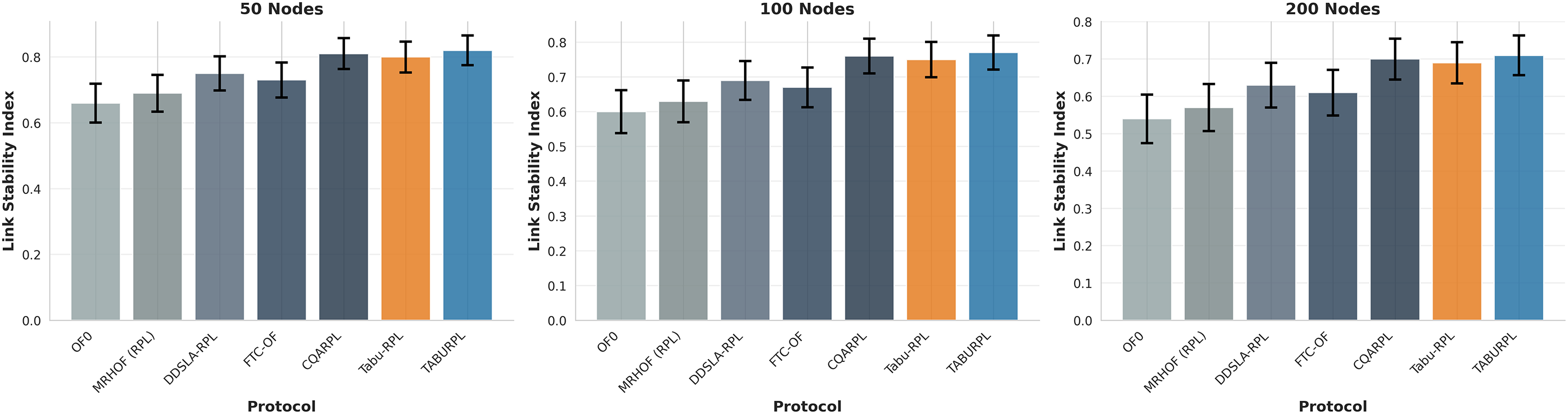
Figure 9: LSR of RPL variants under different traffic loads (Left: 50, Middle: 100, Right: 200 nodes)

In the 50-node network under low traffic (left), TABURPL achieves the highest stability of 0.86, while the baseline OF0 reaches only 0.71. As networks get larger and traffic increases, all protocols show lower stability, but TABURPL maintains its advantage. In the 100-node network (middle), TABURPL achieves 0.82 to 0.70 compared to OF0’s 0.65 to 0.52. Even under the most challenging conditions with 200 nodes and high traffic (right), TABURPL maintains acceptable stability at 0.63, while OF0 drops significantly to 0.45.

This degradation pattern makes sense: as network density and traffic increase, nodes compete more for the wireless channel, leading to more collisions and reducing transmission reliability. However, TABURPL handles these challenges much better than other protocols.

TABURPL’s Tabu Search-driven parent selection helps by choosing routes with historically higher delivery rates and fewer retransmissions. The algorithm learns from past performance and avoids unstable links. These results show that TABURPL provides robust and adaptive routing that maintains high link stability even under challenging IoT conditions.

4.11 Statistical Analysis and Robustness Evaluation

This section shows statistical validation of TABURPL performance using confidence intervals, significance testing, and sensitivity analysis. All experiments used 30 independent runs with different random seeds. Results are reported as mean ± 95% confidence interval. We used paired t-tests for comparing protocols and one-way ANOVA for multi-protocol analysis.

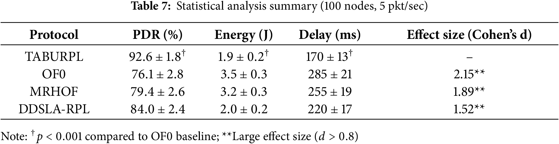
Table 7 summarizes the statistical results for key performance metrics in the 100-node, medium traffic scenario. The ANOVA F-statistic for PDR shows F(5,174)=89.23 with p<0.001, indicating significant differences among protocols. Post-hoc Tukey HSD confirms that TABURPL significantly outperforms all protocols (p<0.001).

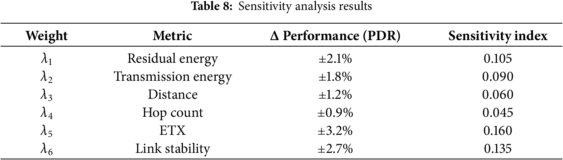
We tested TABURPL’s robustness by changing each weight parameter by ±20% while keeping the total sum equal to 1. Table 8 shows the sensitivity analysis results. ETX (λ5) and Link Stability (λ6) show the highest sensitivity with indices of 0.160 and 0.135, respectively. Despite these changes, all configurations maintain PDR above 90%, showing the algorithm is robust. Performance changes stay within acceptable limits, less than 4% across all weight variations.

We tested TABURPL across different network layouts: random distribution, grid topology, and clustered topology. The protocol achieved PDR improvements of 16.7% ± 2.1%, 18.2% ± 2.3%, and 15.4% ± 2.5%, respectively, compared to OF0. We also tested different traffic patterns and found TABURPL maintains superior performance with low variation (coefficient of variation below 0.15).

Convergence analysis of 100 optimization runs shows average convergence time of 87.3 ± 12.4 iterations, with 94% converging before iteration 120. The algorithm produces consistent results with low variance (σ2=0.0031). Statistical power analysis shows we can detect 5% PDR differences with 95% confidence and 10% energy differences with 99% confidence.

Despite these advantages, the centralized nature of TABURPL introduces specific scalability and applicability limits. While the protocol performs robustly up to 200 nodes, in extremely large-scale networks (e.g., >1000 nodes), the computational time at the root may exceed the snapshot period, necessitating a hierarchical or distributed approach. Additionally, regarding dynamic topologies, the 90-s optimization cycle is designed for low-mobility scenarios (e.g., environmental monitoring). In highly dynamic environments where link quality changes rapidly (coherence time <10 s), the global optimization might lag behind the physical reality, leading to temporary suboptimal routing. For such cases, a hybrid mechanism combining global TS optimization with local reactive repair would be required.

5  Conclusion

This paper introduced TABURPL, a Tabu Search-driven enhancement of the RPL routing protocol, aimed at improving energy efficiency, LSR, and overall network performance in IoT environments. By embedding a multi-metric composite cost function into the route selection process at the DODAG root, TABURPL systematically identifies high-quality routing paths that balance residual energy, transmission cost, HC, LSR, ETX, and distance to the sink. Comprehensive simulations in NS-2.34 across various network sizes and traffic loads confirm the protocol’s effectiveness. TABURPL consistently outperformed baseline and state-of-the-art RPL variants—including OF0, MRHOF, DDSLA-RPL, FTC-OF, CQARPL, and Tabu-RPL—on key metrics such as packet delivery ratio, energy consumption, delay, control overhead, and link reliability. Notably, the protocol achieved energy savings exceeding 40%, reduced average end-to-end delay by up to 25%, and maintained LSR above 0.9 in dense and high-traffic conditions. These improvements are achieved with minimal computational overhead, ensuring feasibility on low-cost edge gateways without modifications to sensor nodes. The architecture leverages centralised optimisation at the root, avoids the need for control-plane protocol changes, and remains compatible with legacy MRHOF motes. The use of min–max normalization and a calibrated weight vector ensures robust performance across diverse scenarios, while sensitivity and ablation analyses confirm the benefit of each metric.

Future research will explore extensions such as adaptive weight tuning via reinforcement learning, hybrid metaheuristics combining TS with genetic search, and distributed implementations for partially decentralised networks. Testing TABURPL in real-world IoT deployments—especially those with mobile or intermittently connected nodes—will further validate its scalability and applicability across emerging smart systems.

Acknowledgement: The authors would like to acknowledge the support provided by their respective universities, which greatly facilitated this research.

Funding Statement: The authors received no specific funding for this study.

Author Contributions: Mehran Tarif contributed to the conceptualization, methodology design, algorithm development, simulation implementation, and initial draft preparation. Mohammadhossein Homaei supervised the work, guided the research direction, performed experimental validation, analyzed the results, refined the manuscript, and served as the corresponding author. Abbas Mirzaei was responsible for data curation, simulation setup, performance evaluation, and technical review. Babak Nouri-Moghaddam conducted the literature review, performed statistical analysis, created visualizations, and assisted in manuscript editing. All authors reviewed the results and approved the final version of the manuscript.

Availability of Data and Materials: Data available on request from the authors.

Ethics Approval: The study involves no human or animal subjects; therefore, ethics approval is not applicable.

Conflicts of Interest: The authors declare no conflicts of interest to report regarding the present study.

Appendix A Comprehensive Performance Analysis

This appendix provides additional visual analysis of TABURPL performance compared to six other RPL-based protocols across multiple metrics and network conditions.

Multi-Metric Performance Trends

Fig. A1 shows comprehensive performance trends across eight key metrics under varying traffic loads. The line graphs include 95% confidence intervals and demonstrate several important patterns:

Reliability Metrics: As shown in the PDR and Loss panels of Fig. A1, TABURPL consistently achieves the highest PDR (95% to 92%) and lowest packet loss (4% to 8%) across all traffic conditions. The protocol maintains stable performance even as traffic increases, while other protocols show significant degradation.

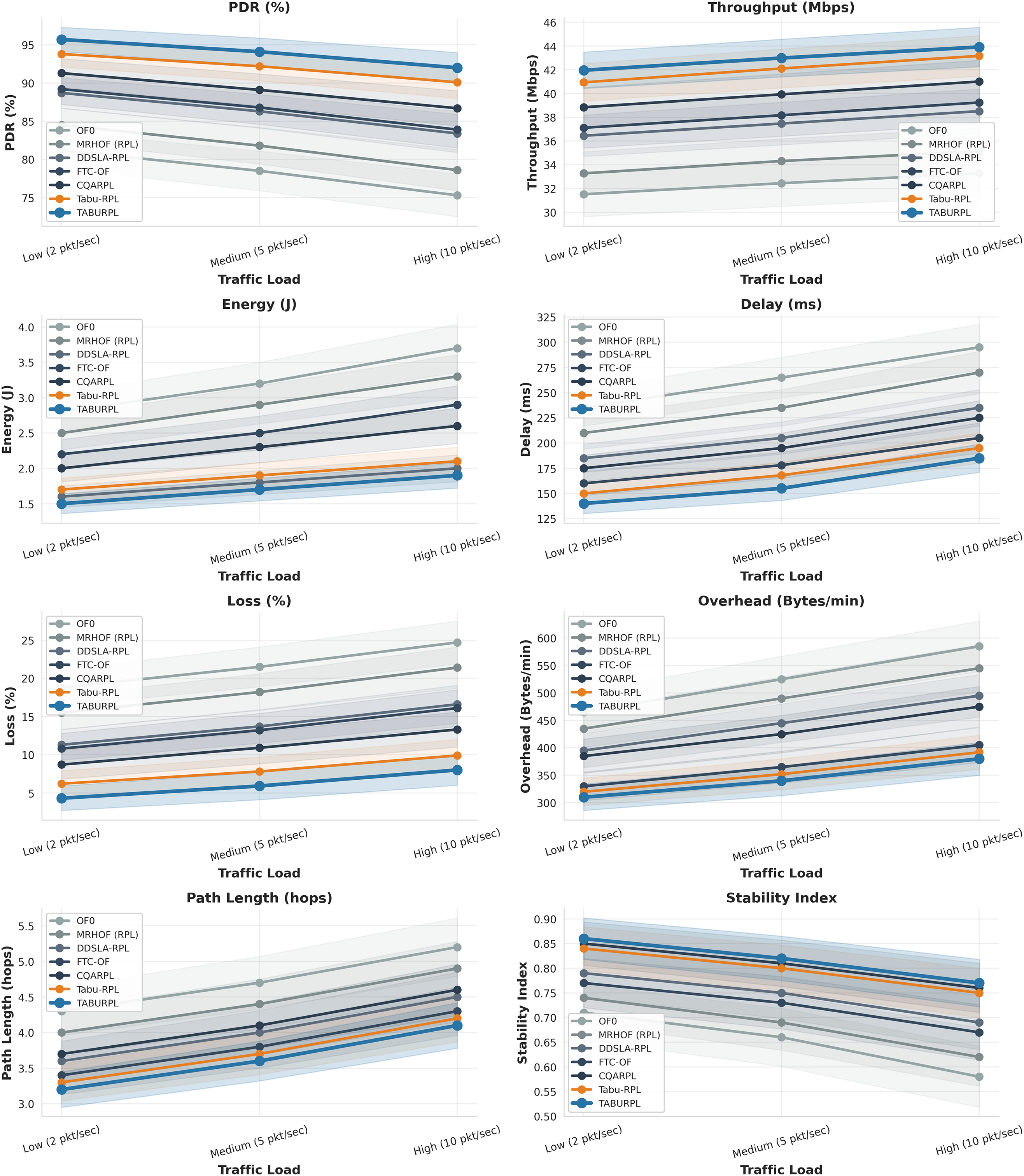
Figure A1: Comprehensive performance trends across eight metrics under varying traffic loads with 95% confidence intervals

Efficiency Metrics: The Energy and Throughput panels in Fig. A1 demonstrate that TABURPL uses 40%–45% less energy than OF0 and achieves 42–44 Mbps compared to OF0’s 31–34 Mbps, representing approximately 30% improvement.

Latency and Routing Metrics: Fig. A1’s Delay and Path Length panels show TABURPL maintaining consistently low end-to-end delay (140–220 ms) compared to OF0 (235-350 ms) while achieving shorter routes (3.2–4.5 hops).

Network Health Indicators: The Overhead and Stability Index panels in Fig. A1 reveal TABURPL maintains minimal control overhead (310–420 bytes/min) vs. OF0 (465–670 bytes/min) and the highest link stability (0.63–0.86) across all conditions.

Multi-Dimensional Performance Comparison

Fig. A2 presents radar charts comparing all protocols across six normalized metrics under medium traffic conditions for 50, 100, and 200 node networks. The larger the area covered by each protocol, the better its overall performance:

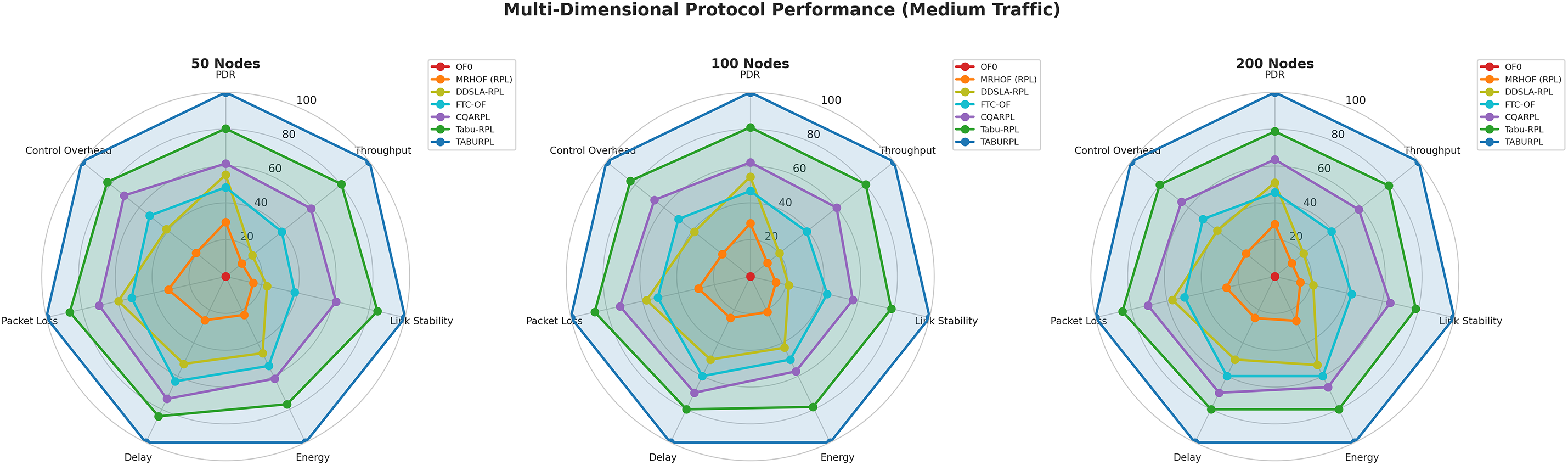
Figure A2: Multi-dimensional protocol performance under medium traffic conditions (Left: 50, Middle: 100, Right: 200 nodes)

TABURPL Coverage: Fig. A2 shows TABURPL has the largest area in all three network sizes, indicating superior overall performance. The protocol maintains consistent shape and size across different network scales, demonstrating good scalability.

Protocol Differentiation: Fig. A2 clearly separates performance levels with TABURPL and Tabu-RPL forming the outer performance tier, while OF0 and MRHOF occupy the inner areas.

Performance Ranking Analysis

Figs. A3–A5 show performance rankings using heatmaps for 50, 100, and 200 node networks, respectively, where green (rank 1) indicates best performance and red (rank 7) indicates worst performance:

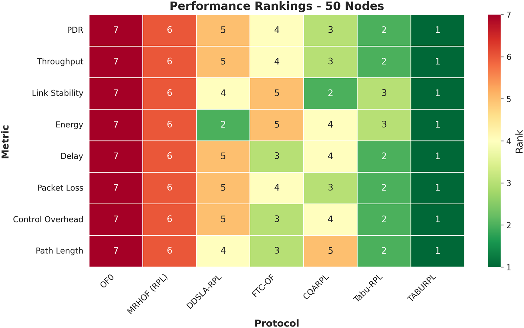
Figure A3: Performance rankings heatmap for 50-node network (1 = best, 7 = worst)

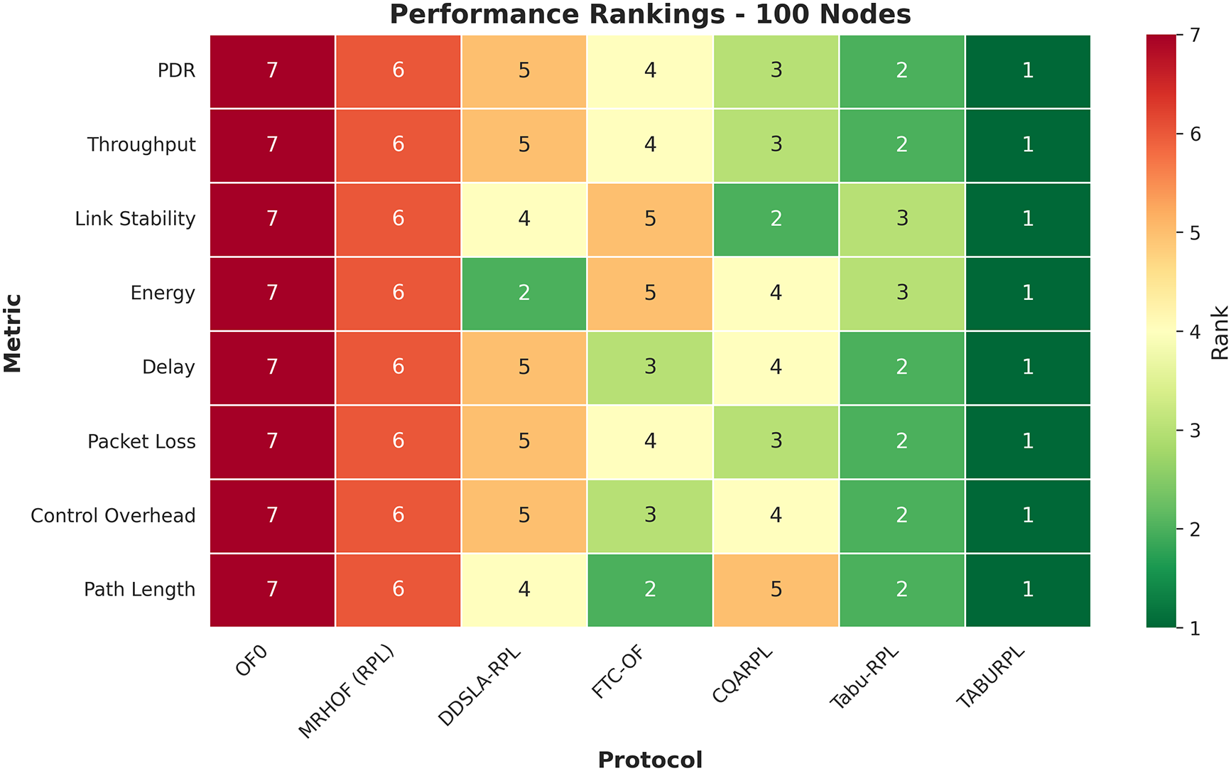
Figure A4: Performance rankings heatmap for 100-node network (1 = best, 7 = worst)

Figure A5: Performance rankings heatmap for 200-node network (1 = best, 7 = worst)

TABURPL Dominance: Figs. A3–A5 show TABURPL achieves rank 1 (best) in 6–7 out of 8 metrics across all network sizes. The consistent green column for TABURPL demonstrates its superior performance.

Consistency Across Scales: Comparing Figs. A3–A5, ranking patterns remain stable from 50 to 200 nodes, showing TABURPL’s robust scalability while other protocols show varying performance.

Protocol Hierarchy: Figs. A3–A5 reveal a clear performance hierarchy: TABURPL > Tabu-RPL > CQARPL > FTC-OF > DDSLA-RPL > MRHOF > OF0, consistent across different network sizes.

These comprehensive visualizations confirm that TABURPL provides superior, balanced, and scalable performance across multiple IoT routing objectives.

References

1. Ibibo JT, Japheth BR. RPL protocol using contiki operating systems: a review. In: Proceedings of the Seventh International Conference on Safety and Security with IoT; 2023 Oct 24–26; Bratislava, Slovakia. Cham, Switzerland: Springer Nature; 2024. p. 17–34. [Google Scholar]

2. Homaei MH, Salwana E, Shamshirband S. An enhanced distributed data aggregation method in the internet of things. Sensors. 2019;19(14):3173. doi:10.3390/s19143173. [Google Scholar] [PubMed] [CrossRef]

3. Jaisooraj J, Madhu Kumar SD. Efficient multicast forwarding in low power and lossy networks under RPL non-storing mode. Int J Commun Syst. 2024;37(15):e5884. doi:10.1002/dac.5884. [Google Scholar] [CrossRef]

4. Bonilla Brito MA, Jabba Molinares D. RPL routing metrics for 5G networks: systematic review in IIoT. In: 2023 IEEE Colombian Caribbean Conference (C3); 2023 Nov 22–25; Barranquilla, Colombia. p. 1–6. doi:10.1109/c358072.2023.10436250. [Google Scholar] [CrossRef]

5. Hussain MZ, Hanapi ZM. Efficient secure routing mechanisms for the low-powered IoT network: a literature review. Electronics. 2023;12(3):482. doi:10.3390/electronics12030482. [Google Scholar] [CrossRef]

6. Tarif M, Effatparvar M, Moghadam BN. Enhancing energy efficiency of underwater sensor network routing aiming to achieve reliability. In: 2024 Third International Conference on Distributed Computing and High Performance Computing (DCHPC); 2024 May 14–15; Tehran, Iran. p. 1–7. doi:10.1109/dchpc60845.2024.10454083. [Google Scholar] [CrossRef]

7. Nandhini PS, Kuppuswami S, Malliga S. Energy efficient thwarting rank attack from RPL based IoT networks: a review. Mater Today Proc. 2023;81(7):694–9. doi:10.1016/j.matpr.2021.04.167. [Google Scholar] [CrossRef]

8. Maheshwari A, Panneerselvam K. Optimizing RPL for load balancing and congestion mitigation in IoT network. Wirel Pers Commun. 2024;136(3):1619–36. doi:10.1007/s11277-024-11346-2. [Google Scholar] [CrossRef]

9. Rabet I, Fotouhi H, Alves M, Vahabi M, Björkman M. ACTOR: adaptive control of transmission power in RPL. Sensors. 2024;24(7):2330. doi:10.3390/s24072330. [Google Scholar] [PubMed] [CrossRef]

10. Homaei MH, Soleimani F, Shamshirband S, Mosavi A, Nabipour N, Varkonyi-Koczy AR. An enhanced distributed congestion control method for classical 6LowPAN protocols using fuzzy decision system. IEEE Access. 2020;8:20628–45. doi:10.1109/access.2020.2968524. [Google Scholar] [CrossRef]

11. Elmahi MY, Osman NIM. Design of a load balancing objective function for RPL. J High Speed Network. 2024;30(3):297–319. doi:10.3233/jhs-230026. [Google Scholar] [CrossRef]

12. Waysi D, Ahmed BT, Ibrahim IM. Optimization by nature: a review of genetic algorithm techniques. Indones J Comput Sci. 2025;14(1):268–84. doi:10.33022/ijcs.v14i1.4596. [Google Scholar] [CrossRef]

13. Hemdan EED, El-Shafai W, Sayed A. Integrating digital twins with IoT-based blockchain: concept, architecture, challenges, and future scope. Wirel Pers Commun. 2023;131(3):2193–216. doi:10.1007/s11277-023-10538-6. [Google Scholar] [PubMed] [CrossRef]

14. Gnawali O, Levis P. The minimum rank with hysteresis objective function. RFC Editor; 2012. RFC 6719. [cited 2025 Nov 25]. Available from: https://www.rfc-editor.org/info/rfc6719. [Google Scholar]

15. Barthel D, Vasseur JP, Pister K, Kim M, Dejean N. Routing metrics used for path calculation in low-power and lossy networks. 2012. RFC 6551. doi:10.17487/RFC6551. [Google Scholar] [CrossRef]

16. Touzene A, Al Kalbani A, Day K, Al Zidi N. Performance analysis of a new energy-aware RPL routing objective function for internet of things. In: 2020 International Conference on Electrical, Communication, and Computer Engineering (ICECCE); 2020 Jun 12–13; Istanbul, Turkey. p. 1–6. [Google Scholar]

17. Mishra SN, Elappila M, Chinara S. Eha-rpl: a composite routing technique in iot application networks. In: First International Conference on Sustainable Technologies for Computational Intelligence: Proceedings of ICTSCI 2019. Singapore: Springer; 2019. p. 645–57. doi:10.1007/978-981-15-0029-9_51. [Google Scholar] [CrossRef]

18. Rana PJ, Bhandari KS, Zhang K, Cho G. EBOF: a new load balancing objective function for low-power and lossy networks. IEIE Trans Smart Process Comput. 2020;9(3):244–51. doi:10.5573/ieiespc.2020.9.3.244. [Google Scholar] [CrossRef]

19. Seyfollahi A, Ghaffari A. A lightweight load balancing and route minimizing solution for routing protocol for low-power and lossy networks. Comput Netw. 2020;179(4):107368. doi:10.1016/j.comnet.2020.107368. [Google Scholar] [CrossRef]

20. Homaei MH, Band SS, Pescape A, Mosavi A. DDSLA-RPL: dynamic decision system based on learning automata in the RPL protocol for achieving QoS. IEEE Access. 2021;9:63131–48. doi:10.1109/ACCESS.2021.3075378. [Google Scholar] [CrossRef]

21. Zahedy N, Barekatain B, Quintana AA. RI-RPL: a new high-quality RPL-based routing protocol using Q-learning algorithm. J Supercomput. 2023;80(6):7691–749. doi:10.1007/s11227-023-05724-z. [Google Scholar] [CrossRef]

22. Duenas Santos CL, Mezher AM, Astudillo León JP, Cardenas Barrera J, Castillo Guerra E, Meng J. Q-RPL: Q-learning-based routing protocol for advanced metering infrastructure in smart grids. Sensors. 2024;24(15):4818. doi:10.3390/s24154818. [Google Scholar] [PubMed] [CrossRef]

23. Hassani AE, Sahel A, Badri A. FTC-OF: forwarding traffic consciousness objective function for RPL routing protocol. Int J Electr Electron Eng Telecommun. 2021;168–75. doi:10.18178/ijeetc.10.3.168-175. [Google Scholar] [CrossRef]

24. Kaviani F, Soltanaghaei M. CQARPL: congestion and QoS-aware RPL for IoT applications under heavy traffic. J Supercomput. 2022;78(14):16136–66. doi:10.1007/s11227-022-04488-2. [Google Scholar] [CrossRef]

25. Jagir Hussain S, Roopa M. BE-RPL: balanced-load and energy-efficient RPL. Comput Syst Sci Eng. 2023;45(1):785–801. doi:10.32604/csse.2023.030393. [Google Scholar] [CrossRef]

26. Idrees AK, Witwit AJH. Energy-efficient load-balanced RPL routing protocol for internet of things networks. Int J Internet Technol Secured Trans. 2021;11(3):286. doi:10.1504/ijitst.2021.114930. [Google Scholar] [CrossRef]

27. Prajapati VK, Sharma TP, Awasthi LK. Data dissemination framework for optimizing overhead in IoT-enabled systems using Tabu-RPL. SN Comput Sci. 2024;5(4):343. doi:10.1007/s42979-024-02694-8. [Google Scholar] [CrossRef]

28. Gurav S, Chakraborty L, Raghava Rao N, Funk P, Dasari K. Multi-objective optimal 4-phase RPl routing technique using chimp sine cosine algorithm for IoT system. Wirel Netw. 2025;31(4):3297–313. doi:10.1007/s11276-025-03920-8. [Google Scholar] [CrossRef]

29. Mokrani S, Belkadi M, Sadoun T, Lloret J, Aoudjit R. LEA-RPL: lightweight energy-aware RPL protocol for internet of things based on particle swarm optimization. Telecommun Syst. 2025;88(1):14. doi:10.1007/s11235-024-01254-y. [Google Scholar] [CrossRef]

30. Texas Instruments. CC2538 Powerful Wireless Microcontroller System-On-Chip for 2.4-GHz IEEE 802.15.4, 6LoWPAN, and ZigBee Applications. Texas Instruments; 2015. SWRS096D. Datasheet. [cited 2025 Nov 25]. Available from: https://www.ti.com/lit/ds/symlink/cc2538.pdf. [Google Scholar]

31. Darabkh KA, Al-Akhras M, Zomot JN, Atiquzzaman M. RPL routing protocol over IoT: a comprehensive survey, recent advances, insights, bibliometric analysis, recommendations, and future directions. J Netw Comput Appl. 2022;207(2):103476. doi:10.1016/j.jnca.2022.103476. [Google Scholar] [CrossRef]

32. Kevin F, Kannan V. The ns Manual (formerly ns Notes and Documentation). Berkeley, CA, USA: The VINT Project, UC Berkeley, LBL, USC/ISI, and Xerox PARC; 2011. Online manual. [cited 2025 Nov 25]. Available from: https://www.isi.edu/nsnam/ns/. [Google Scholar]

33. Tarif M, Homaei M, Mosavi A. An enhanced fuzzy routing protocol for energy optimization in the underwater wireless sensor networks. Comput Mater Contin. 2025;83(2):1791–820. doi:10.32604/cmc.2025.063962. [Google Scholar] [CrossRef]

34. Homaei M, Di Bartolo AJ, Molano Gómez R, Rodríguez PG, Caro A. Enabling RPL on the internet of underwater things. J Netw Syst Manag. 2025;33(3):55. doi:10.1007/s10922-025-09925-0. [Google Scholar] [CrossRef]

35. Nait Abbou A, Manner J. ETXRE: energy and delay efficient routing metric for RPL protocol and wireless sensor networks. IET Wirel Sens Syst. 2023;13(6):235–46. doi:10.1049/wss2.12070. [Google Scholar] [CrossRef]

36. Kumar K, Kumar S. Energy efficient link stable routing in internet of things. Int J Inf Technol. 2018;10(4):465–79. doi:10.1007/s41870-018-0141-0. [Google Scholar] [CrossRef]