An Integrated Attention-BiLSTM Approach for Probabilistic Remaining Useful Life Prediction

1  Introduction

In modern industrial systems, Prognostics and Health Management (PHM) plays a crucial role in maintaining equipment functionality, reducing failure rates, and minimizing maintenance costs. By leveraging advanced sensing technologies, PHM collects operational data from equipment, which is then processed through techniques such as data analysis and information fusion to assess real-time health status and predict potential failures. These insights support managerial decision-making regarding maintenance actions [1,2].

During operation, equipment is subject to performance degradation due to various external destructive factors, ultimately leading to failure. Research on Remaining Useful Life (RUL) focuses on analyzing performance degradation characteristics to forecast mechanical failures and prevent potential accidents. The total lifespan of equipment refers to the duration from its initial normal state through progressive degradation until functional failure occurs. RUL is defined as the expected operational time from a given inspection point until failure occurs, under the condition of no maintenance. RUL prediction models utilize degradation trajectories and integrate current and historical data to estimate the remaining operational life effectively. However, conventional techniques such as Convolutional Neural Networks (CNNs) and Long Short-Term Memory (LSTM) networks are often applied directly to raw signals that contain random noise, which can significantly impair their performance. Given the importance of temporal features, Bidirectional Long Short-Term Memory (BiLSTM) has been widely adopted in RUL prediction due to its superior capability in capturing temporal dependencies [3,4]. As illustrated in Fig. 1, which displays four randomly selected engine operation sequences from the C-MAPSS dataset, noticeable noise is commonly present in the raw temporal signals. Such noise induces substantial signal fluctuations and leads to highly degraded encoded sequence information, thereby reducing RUL prediction accuracy.

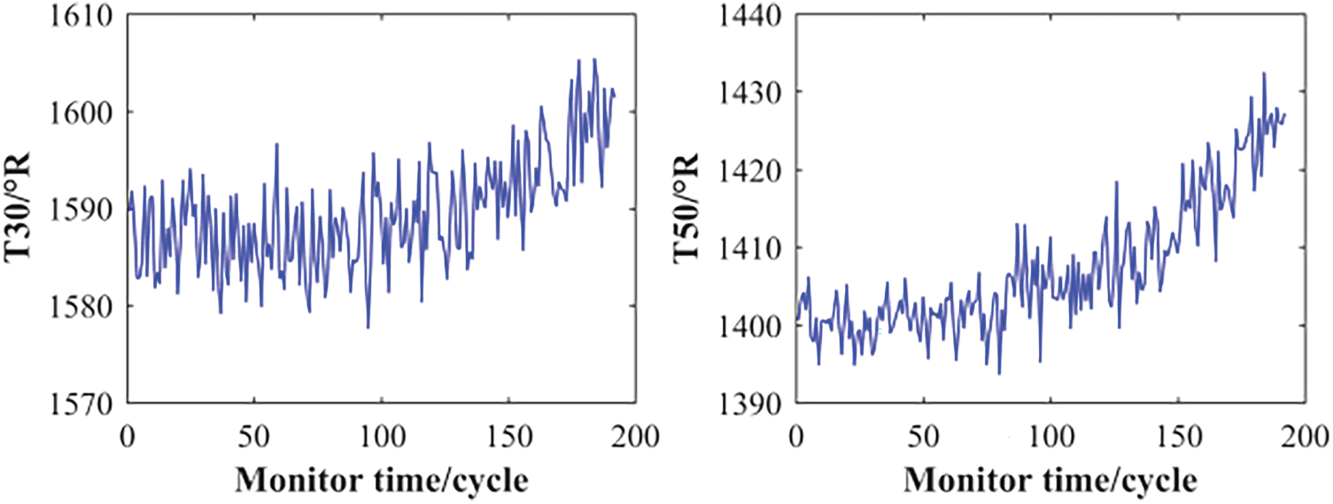
Figure 1: Raw time-series signals with widespread random noise

Although BiLSTM networks and attention mechanisms have been extensively explored, most existing studies only focus on achieving more accurate point predictions [5,6]. In contrast, this study aims to address the paradigm shift from point prediction to probabilistic distribution prediction. We would like to emphasize that the proposed Kernel Density Estimation (KDE) integration framework can convert multiple deterministic prediction points output by the deep learning model into an interpretable probability distribution. This constitutes a key innovation that distinguishes our work from previous efforts, which merely improved network structures to enhance point prediction accuracy.

To address these issues, this study proposes a deep network integrating BiLSTM with an attention mechanism and a prediction framework based on KDE. This combined approach enables comprehensive training and testing of real-time feature data from equipment degradation, thereby providing more scientific and accurate RUL predictions. This work seeks to promote the broader application of deep learning technologies in PHM and enhance equipment reliability and operational safety. By shifting the paradigm from deterministic point estimation to probabilistic risk assessment, the proposed framework equips managers with not only a predicted RUL but also a clear understanding of the associated uncertainty, thereby enabling more scientific and cost-effective maintenance decisions.

2  Related Work

Addressing the complexity of industrial AI, machine learning has emerged as a vital tool for fault diagnosis and smart factory health management. Key contributions collectively underscore this trend: Raouf et al. [7] provided a systemic overview of PHM in smart factories, while Kumar et al. [8] reviewed algorithmic strategies for robotics and machinery. On the implementation front, Raouf et al. proposed a fault classification system using motor current analysis [9] and later a feature aggregation network for detecting bearing faults in industrial robots [10]. RUL prediction aims to estimate the operational lifespan remaining for critical components of equipment by analyzing degradation trajectories and leveraging time-series data from multiple sensors (e.g., vibration signals). Conventional RUL prediction approaches can be broadly categorized into two groups: physics-based models and data-driven methods [11,12].

In recent years, deep learning-based methods have gained widespread adoption. These approaches treat the equipment as a black box, automatically learning high-level abstract features from raw time-series signals through multi-type and multi-dimensional neural network layers. This eliminates the need for manual feature engineering, making them particularly suitable for complex systems with high-dimensional and unstructured operational data. Common architectures include CNN-based, LSTM-based [3,4], and TCN-based [13–15] models. In practice, hybrid models combining multiple neural networks are often developed to enhance performance. For instance, Zha et al. [13] proposed an RUL prediction model integrating XGBoost for feature extraction and an improved temporal convolutional network. He et al. [16] developed a bearing RUL prediction model using a dual correlation adaptive gated graph convolutional network (DCAGGCN). Liao et al. [17] introduced an LSTM-based feedforward neural network (LSTM-FNN) with a bootstrap method (LSTMBS) for uncertainty prediction in RUL estimation. Xiang et al. [18] developed a multicellular LSTM (MCLSTM) structure based on layer-partitioned and multi-cell units, establishing a deep learning framework for RUL prediction. Chen et al. [19] proposed a novel approach to improve the accuracy of bearing RUL prediction by employing a prototypical network to identify abrupt changes in health states. Yu et al. [20] integrated similarity curve matching into a bidirectional recurrent network-based autoencoder scheme for RUL estimation. Zhang et al. [21] devised a bidirectional gated recurrent unit with a temporal self-attention mechanism (BiGRU-TSAM), which assigns self-learned weights to each considered time instance for RUL prediction. Al-Dulaimi et al. [22] presented a hybrid deep neural network (HDNN) framework, noted as the first to concurrently integrate two DL models in parallel.

Currently, numerous studies have integrated deep learning networks with attention mechanisms [23–25]. Han et al. [26] proposed a novel parallel convolutional LSTM dual-attention (PCLD) model incorporating both long short-term memory networks and a dual-attention mechanism. Zhang et al. [27] combined slow feature analysis-assisted attention with a dual-LSTM network to enhance feature representation. Liu et al. [28] adopted a two-phase training strategy: the model is first pre-trained to capture general equipment operating states, and then fine-tuned on a single dataset to adapt to specific working conditions, while a sequential feature attention mechanism is employed to integrate multi-dimensional time-series data.

Despite advances in deep learning for RUL prediction, existing methods still struggle with two key challenges in real industrial settings: limited robustness under complex noise and fluctuating conditions, which obscures true degradation trends, and the inability to shift from deterministic point estimates to probabilistic uncertainty quantification, leaving prediction reliability unassessed.

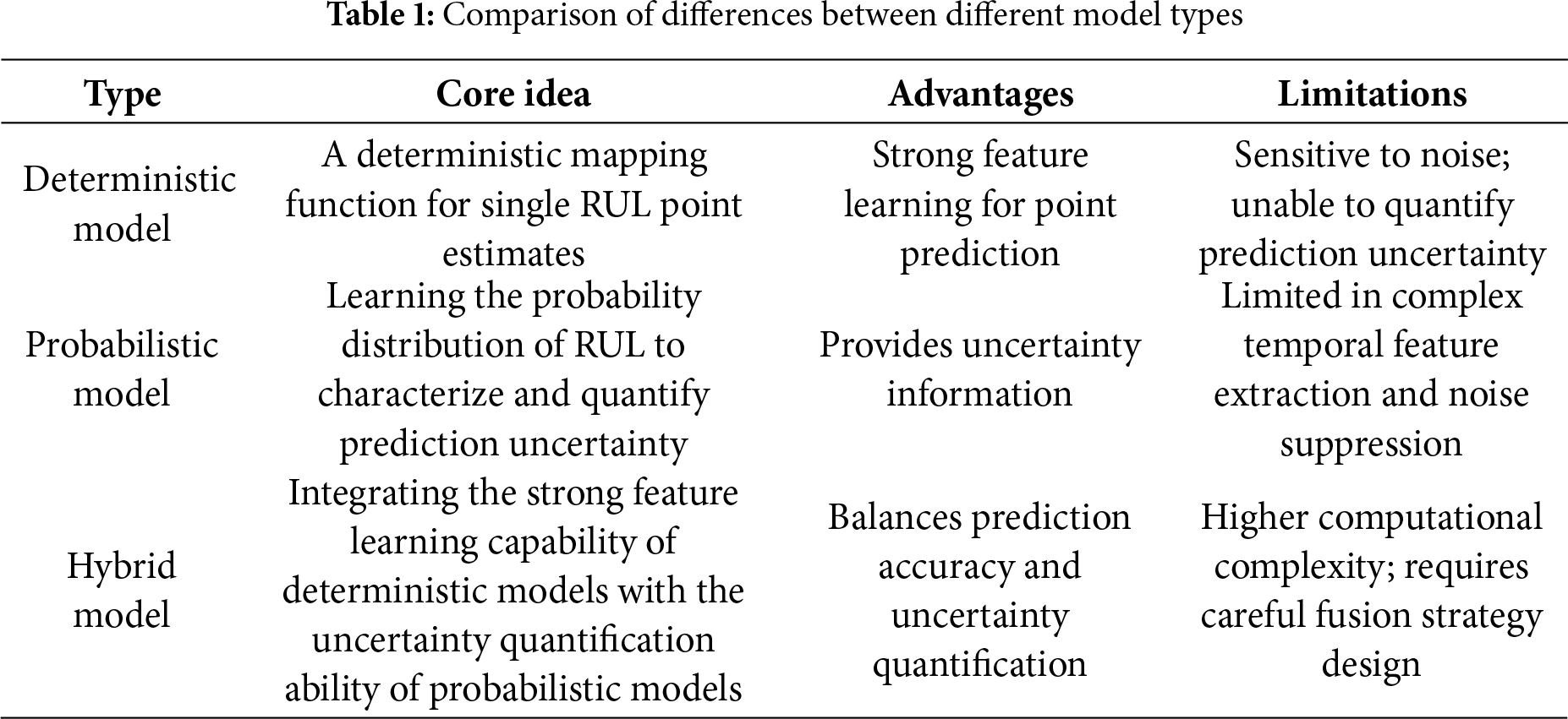
To critically synthesize and analyze the work covered in existing literature, this study summarizes the differences between deterministic models, probabilistic models, and hybrid models in terms of core ideas, advantages, limitations, and representative methods, as presented in Table 1.

This paper proposes an integrated deep learning framework for the probabilistic prediction of RUL of mechanical equipment. At the conceptual level, this work shifts the paradigm from deterministic point estimation to probabilistic distribution prediction. The key innovation lies in integrating KDE to convert multiple deterministic model outputs into a complete and interpretable probability density function, thereby transforming the prediction from a single value into a quantified uncertainty. On the practical front, our method provides a full probability distribution that enables risk-informed decision-making, moving beyond a single point estimate of unknown reliability. This allows maintenance strategies to evolve from simplistic threshold-based triggers to dynamic, risk-based planning, offering significant practical value for optimizing operational economics and safety. The main innovations can be summarized as follows:

An Attention- BiLSTM architecture

The proposed Attention-BiLSTM architecture leverages bidirectional layers to capture both historical and future context, overcoming the limitation of unidirectional models in learning long-term, bidirectional dependencies. An integrated additive attention mechanism automatically prioritizes critical degradation phases while suppressing irrelevant noise.

A probabilistic prediction framework based on KDE

This framework generates a set of prediction samples for KDE by performing multiple samplings from the posterior distribution of network weights. Applying KDE to these generated samples yields a full probability density distribution of the RUL. This synergistic design ensures stable model optimization while constituting an end-to-end probabilistic prediction solution.

A shift from deterministic point prediction to probabilistic distribution prediction

While most existing studies focus on improving point prediction accuracy of RUL through network structure enhancements, the proposed probabilistic framework not only provides a point estimate of RUL but also enables the quantification of prediction uncertainty, offering a reliable basis for risk-informed maintenance decision-making.

3  Methodology

3.1 Deep Neural Network Based on BiLSTM with Attention Mechanism

The workflow of the proposed probabilistic RUL prediction framework is illustrated in Fig. 2. The figure clearly depicts the end-to-end data flow, starting from the input of raw multi-sensor time-series data, followed by data preprocessing and sliding window segmentation, bidirectional feature encoding via the BiLSTM layer, calculation of key time-step weights by the attention mechanism layer, output of deterministic predictions through the fully connected layer, activation of Monte Carlo Dropout for multiple forward samplings to model uncertainty, and finally fusion of all sampling points using KDE to generate a probability density distribution. This distribution provides a basis for risk quantification in decision-making.

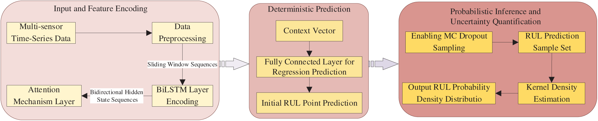
Figure 2: Flowchart of the probabilistic RUL PREDICTION FRAMEWORK

To address the challenge of predicting the RUL of equipment, a deep fusion network incorporating a BiLSTM architecture is proposed, with the aim of enhancing the extraction of temporal features and complex patterns. The core idea leverages the bidirectional temporal modeling capability of BiLSTM to fully capture contextual relationships in time-series data through the integration of both forward and backward directions. This mechanism overcomes the limitations of traditional unidirectional LSTM in modeling long-range dependencies and significantly improves the capture of dynamic correlations within time-series data. The workflow is illustrated in Fig. 3.

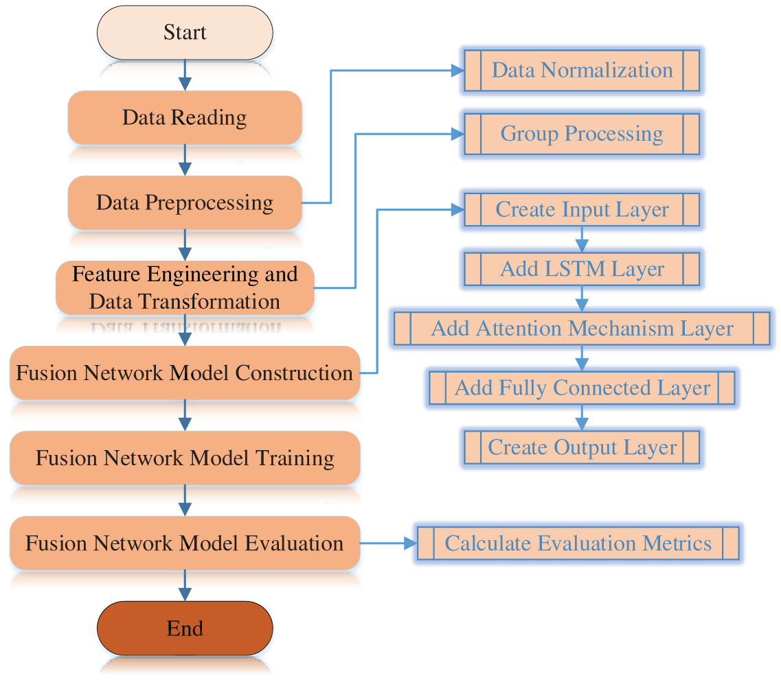
Figure 3: Workflow diagram of fusion network model

BiLSTM has demonstrated strong capabilities in capturing sequential dependencies. The computational process for the forward module of the model is given as follows [3]:

i→(t)=σ(ω→iix→t+ω→hih→(t−1)+bt→)(1)

f→(t)=σ(ω→ifx→t+ω→hfh→(t−1)+b→f)(2)

g→(t)=tanh⁡(ω→igx→t+ω→hgh→(t−1)+b→g)(3)

o→(t)=σ(ω→iox→t+ω→hoh→(t−1)+b→o)(4)

c→(t)=f→(t)⊙c→(t−1)+i→(t)⊙g→(t)(5)

h→(t)=o→(t)⊙tanh⁡c→(t)(6)

Similarly, formulation of the backward part of the BiLSTM albeit with a reversed temporal sequence:

i←(t)=σ(ω←iix←t+ω←hih←(t−1)+b←t)(7)

f←(t)=σ(ω←ifx←t+ω←hfh←(t−1)+b←f)(8)

g→(t)=tanh⁡(ω→igx→t+ω→hgh→(t−1)+b→g)(9)

o←(t)=σ(ω←iox←t+ω←hoh←(t−1)+b←o)(10)

c←(t)=f←(t)⊙c←(t−1)+i←(t)⊙g←(t)(11)

h←(t)=o←(t)⊙tanh⁡c←(t)(12)

In Eqs. (1)–(12), i(t), f(t), g(t), and o(t) represent the input gate, forget gate, candidate cell state, and output gate at time t, respectively; h(t) and c(t) denote the hidden state and cell state at time t, respectively; σ denotes the sigmoid function, ⊙ denotes the Hadamard product, wii, whi, wif, whf, wio, who, wig, whg are learnable weights, bi, bf, bg, bo are bias terms, → indicates the forward direction, and ← indicates the backward direction. The above equations collectively constitute the core computational mechanism of the BiLSTM network. Through a series of differentiable control structures—including the input gate, forget gate, and output gate—the network adaptively manages the state of its internal memory cells. The forget gate f(t) determines how much information to retain from the historical memory cell c(t − 1) based on the current input and the previous hidden state; a value closer to 1 indicates more memory retention. The input gate i(t) works in conjunction with the candidate state g(t) to decide how much new information from the current input should be updated into the memory cell c(t). Finally, the output gate o(t) controls how much information from the current memory cell c(t) is output as the hidden state h(t) and passed to subsequent layers. By processing sequences along both forward and backward time axes, the BiLSTM can integrate contextual information at each time step.

The BiLSTM integrates two oppositely oriented LSTM layers to capture long-term temporal dependencies from bidirectional data. After processing through multiple LSTM layers, the model employs data smoothing to filter out noise interference from the raw input signals, thereby facilitating more accurate extraction of temporal features and improving the precision of RUL prediction. The architecture of the model is illustrated in Fig. 4, and its final output is expressed as follows:

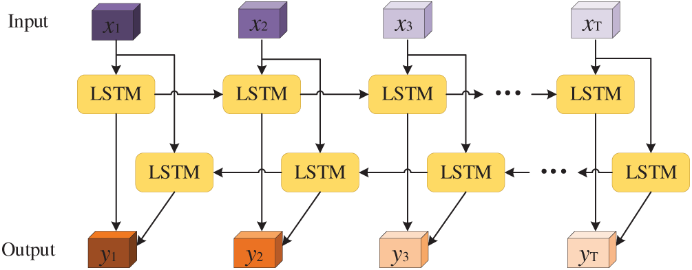
Figure 4: Schematic diagram of the BiLSTM model workflow

h(t)=h→(t)⊕h←(t)(13)

The Additive Attention Layer, a classical implementation of the attention mechanism originally proposed by Bahdanau et al. in 2015 (also referred to as Bahdanau attention), computes the relevance between queries and keys through learnable parameters. Its core idea involves mapping queries and keys to the same dimension via separate linear transformations, followed by an additive operation and a nonlinear activation function to derive the attention weights [29]. For a given input sequence {x1,…,xt}, this encoder produces a forward hidden state sequence {h1→,…,ht→} and a backward hidden state sequence {h1←,…,ht←}. The encoded representation of any element xj is formed by concatenating its corresponding forward and backward hidden states. The attention mechanism contains an alignment model that measures how well the annotation hj from the input suits the hidden state si−1 from the output. The calculation formula is as follows:

eij=vaTtan⁡h(Wasi−1+Uahj)(14)

where Wa∈Rm×m and Ua∈Rm×2m are learnable weight matrix, va∈Rm is a weight vector used to compress to a scalar, and m is the dimension of the attention hidden layer.

The weights are calculated by applying the softmax operation to the alignment scores, and they represent the probability that the input xj is aligned with the output yi. The weight distribution can be obtained by normalizing the scores with softmax.

αij=softmax(eijm)(15)

As output of the attention mechanism, the context vector is calculated as the annotations hj:

Coni=∑j=1Nαijhj(16)

The model in Eq. (14) learns to evaluate the relevance between the hidden state hj (at the j-th time step of the input sequence) and the prediction target for the current prediction task. Subsequently, these scores are normalized into a probability distribution αij via the Softmax function in Eq. (15). Finally, as shown in Eq. (16), the hidden states of all time steps are weighted and summed according to their attention weights, generating a context vector cij that condenses the key information of the sequence.

3.2 KDE-Based Probabilistic RUL Prediction Framework

The innovation of the proposed prediction framework lies in the synergistic mechanism between residual learning and stochastic regularization. The residual pathway enables cross-layer propagation of raw signals through parallel linear transformations, whose mathematical essence establishes a high-speed channel for gradient flow. Experimental results demonstrate that this design effectively mitigates the gradient vanishing problem when handling long-term temporal dependencies in sensor signals. Meanwhile, LayerNorm standardizes the activation values of neurons, maintaining the data distribution of each layer’s output within a stable range. Since each forward propagation effectively samples from the posterior distribution of network weights, the predictive distribution obtained through multiple sampling iterations naturally incorporates model epistemic uncertainty. This elegantly introduces Bayesian inference into conventional neural networks [30] and enables probabilistic outputs without altering the base architecture. The selection of the KDE method is primarily based on two considerations. First, as a non-parametric method, KDE does not require prior assumptions about the distribution shape of predictions, enabling more flexible fitting of complex distribution patterns (e.g., skewed or multimodal distributions) that may occur in real-world data. Second, it offers high computational efficiency, making it particularly suitable for combination with Monte Carlo Dropout sampling and thus more feasible and practical for engineering applications.

Theoretical analysis indicates that the generalization capability of this architecture stems from the synergy of multiple regularization mechanisms: Dropout provides a model averaging effect in deep networks, LayerNorm maintains feature distribution stability, and residual connections ensure optimization feasibility. Each forward pass utilizes a randomly generated Dropout mask, effectively sampling a distinct sub-network from the learned weight posterior. This process yields a discrete set of T prediction points, capturing the epistemic uncertainty arising from model parameters. Residual connections are incorporated after the second BiLSTM layer, with their outputs summed to those of the attention layer to mitigate gradient vanishing in deep networks. Stochastic regularization is implemented via Dropout layers applied after each BiLSTM layer and the first fully-connected layer, with a dropout rate of 0.2 determined through grid search.

For practical decision-making, key quantiles can be easily derived from the probability density distribution to define a predictive confidence interval. By evaluating this failure risk, strategies like condition-based maintenance can be optimized to balance the costs of unexpected downtime against those of premature component replacement. The main workflow is illustrated in Fig. 5.

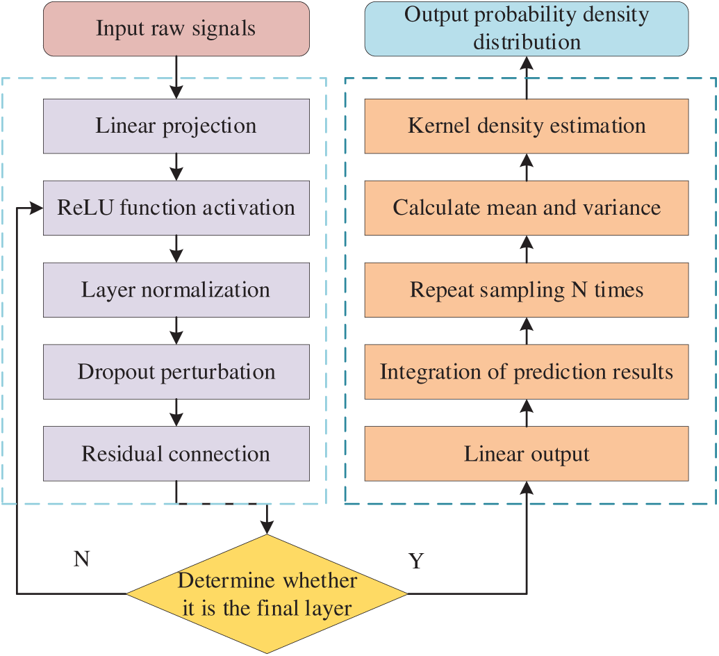
Figure 5: Implementation flowchart of the RUL prediction framework

Following the approach in reference [31], in Bayesian learning, for a given input x*, obtaining its predictive distribution requires marginalizing over all model parameters:

f(y∗|x∗,X,Y)=∫f(y∗|x∗,ω)f(ω|X,Y)dω(17)

where ω={N^k}k=1L denotes the set of random variables for an L-layer model.

To approximate the predictive distribution, T sets of vectors are sampled from a Bernoulli distribution with probability {p1,…,pL}, enabling empirical estimation of the first two moments:

Ef(y∗|x∗)(y∗)≈1T∑t=1Ty^∗(x∗,N^kt,…,N^Lt)(18)

Monte Carlo estimator is referred to as MC-Dropout. In practice, it is equivalent to performing T forward passes through the deep network and averaging the outputs. We provide a novel derivation for this result, which allows us to derive well-founded uncertainty estimates. Empirically, the integration can be approximated by averaging the network weights (i.e., scaling each Wi by pi at test time). Similarly, for regression tasks, the predictive mean and variance can be computed as:

Ef(y∗|x∗)((y∗)T(y∗))≈ς−1ID+1T∑t=1Ty^∗(x∗,N^1t,…,N^Lt)Ty^∗(x∗,N^1t,…,N^Lt)(19)

Varf(y∗|x∗)(y∗)≈ς−1ID+1T∑t=1Ty^∗(x∗,N^1t,…,N^Lt)Ty^∗(x∗,N^1t,…,N^Lt)−Ef(y∗|x∗)(y∗)TEf(y∗|x∗)(y∗)(20)

where the predictive uncertainty is estimated via the sample variance over T forward passes plus the inverse model precision, denoted by ς. Since the model precision is often related to the ratio between learning rate r1 and weight decay r2, we define ς=r1/r2.

This prediction framework utilizes multiple forward passes with Dropout enabled, performing N predictions for each model in the ensemble to approximate Bayesian inference. The final prediction is obtained by aggregating all sampled outputs through averaging, while the resulting probability density distribution reflects the model’s predictive uncertainty. Theoretical studies have demonstrated that residual connections can enhance the optimization behavior of the network. Dropout can be interpreted as a Bayesian approximation of Gaussian processes, with its key advantage lying in the provision of predictive distributions rather than point estimates—this is crucial for risk assessment in RUL prediction applications.

In engineering practice, when applying KDE, an ensemble strategy is adopted: each of the 10 base models performs 100 independent predictions, resulting in a total of 1000 predictive samples. These predictions are processed via KDE to generate probability distribution curves of the RUL. Research indicates that under large-sample conditions, the choice of kernel function has limited influence on the shape of the probability density function. The mathematical formulation can be expressed as follows:

f^(x)=1n∑i=1n1hκ(x−xih)=1n∑i=1n1h2πe−12(x−xih)2(21)

In the Eq. (21), κ represents the Gaussian kernel function, x−xih denotes the normalized distance variable, and h is the bandwidth parameter, which controls the smoothness of the kernel. We adopted the commonly used Scott’s rule to adaptively determine the optimal bandwidth, which provides excellent smoothing for data approximating a normal distribution. The specific formula is h=n−1d+4, where n denotes the number of samples and d represents the dimension.

Unlike deterministic RUL prediction models, the proposed framework employs KDE to model the probability density distribution of the RUL prediction, thereby enabling uncertainty quantification—an essential feature for supporting maintenance decision-making by management.

4  Case Study

4.1 Dataset Description

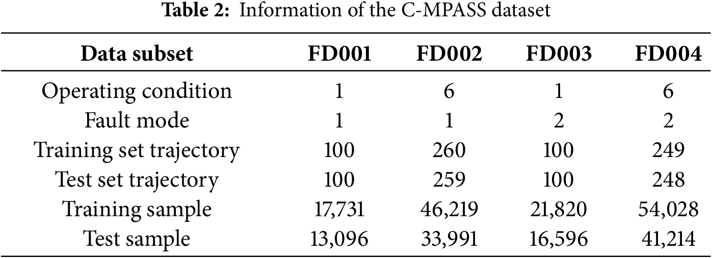
To validate the effectiveness of the proposed RUL prediction method, time-series data from 21 sensors in the C-MAPSS dataset [32] were utilized, with the aircraft engine model illustrated in Fig. 6. These sensors capture measurements such as temperature, pressure, and rotational speed from various locations within the engine. By simulating turbofan engine degradation under diverse conditions and faults, the dataset captures complex performance dynamics. The significant variation in complexity and fault types among its subsets makes them an ideal testbed for a thorough evaluation of model adaptability and generalizability. Detailed information on the four subsets of C-MAPSS is provided in Table 2. As shown in the table, FD002 and FD004 are more complex than the other subsets, containing more training and testing trajectories and involving six different operating conditions. Following the setup in [4], sensor outputs that remain constant throughout the lifecycle—providing no useful information for RUL prediction. Thus, 14 sensor signals were selected for both training and testing, specifically from sensors numbered 2, 3, 4, 7, 8, 9, 11, 12, 13, 14, 15, 17, 20, and 21.

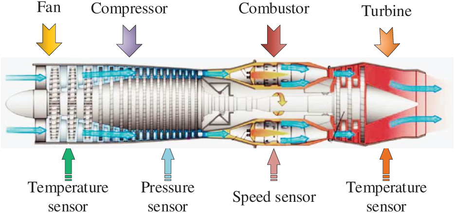
Figure 6: Schematic diagram of the C-MPASS aero-engine model

In accordance with [4], a sliding window of size 30 was applied to segment the sensor data. For sequences shorter than 30 time steps, the segmented data were padded using the first available value. To direct the model’s focus toward the critical degradation phase near failure, the RUL labels in early stages were truncated to a constant value. A sliding step of 1 was adopted to maximize training data utilization by generating a large number of overlapping windows, thereby enriching the training samples. Data normalization, which has been shown to be crucial in RUL prediction, was performed using min-max scaling on all sensor readings, with the maximum RUL value set to 125.

4.2 Network Hyperparameters

The hyperparameter configuration of the proposed deep fusion network reflects a carefully balanced design tailored for time-series regression tasks. The input window length was set to 30 time steps, sufficiently capturing engine degradation trends without introducing excessive noise. The corresponding 14 input features represent the most predictive sensor indicators retained after preprocessing. The hidden architecture comprises two LSTM layers, each with 50 units, providing adequate memory capacity to learn temporal dependencies while controlling model complexity to avoid overfitting. Subsequent fully connected layers consist of 96 and 128 neurons, respectively. This progressively expanding structure facilitates hierarchical feature abstraction, enabling the extraction of high-level patterns from sequential encodings for accurate prediction.

The Adam optimizer was selected for its ability to adaptively adjust the learning rate without manual scheduling. The MSE loss function was used to heavily penalize large prediction errors. An early stopping mechanism with a patience of 10 epochs was employed to terminate training promptly when validation loss ceased to improve and restore the optimal weights, effectively preventing overfitting. A learning rate decay mechanism was also adopted, reducing the learning rate to one-tenth of its original value if no improvement was observed after 5 epochs. For model training, the batch size was set to 32 and the number of training epochs to 100, with all experiments conducted under the TensorFlow framework. Training was performed on a workstation equipped with an NVIDIA RTX 3080 GPU, using an initial learning rate of 0.001 and a learning rate scheduling strategy. The complete training process took approximately 1–1.5 h, with slight variations across different dataset subsets.

4.3 Evaluation Metrics

To validate the effectiveness and reliability of the proposed model, the following evaluation metrics were employed: Root Mean Square Error (RMSE) and Score function.

1.   RMSE: This metric measures the deviation between predicted values and actual values. It is defined as follows:

RMSE=1N∑k=1N(Δk)2(22)

2.   Score: In practical applications, late predictions may lead to more severe consequences than early predictions. To reflect this, the Score function imposes a higher penalty on late predictions compared to early ones. It is calculated as follows:

Score={∑k=1N(eΔk13−1),Δk<0∑k=1N(eΔk10−1),Δk≥0(23)

In Eqs. (22) and (23), Δk=RUL^k−RULk, N represents the number of samples, while RUL^k and RULk denote the predicted and true values of RUL, respectively.

4.4 RUL Prediction Results

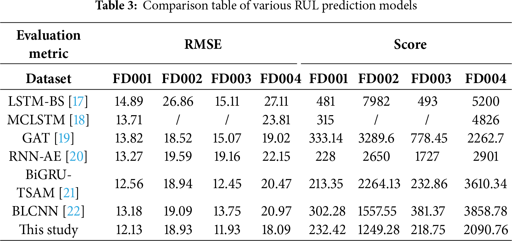
This section presents a comparative analysis between the proposed BiLSTM-based fusion network and several state-of-the-art methods referenced in Table 3, including LSTM-BS [17], MCLSTM [18], GAT [19], RNN-AE [20], BiGRU-TSAM [21], and BLCNN [22]. The BiLSTM-based fusion network demonstrates superior performance over most comparative methods across multiple subsets. Notably, it achieves significant improvements in both RMSE and Score metrics on the more challenging and complex subsets, FD003 and FD004.

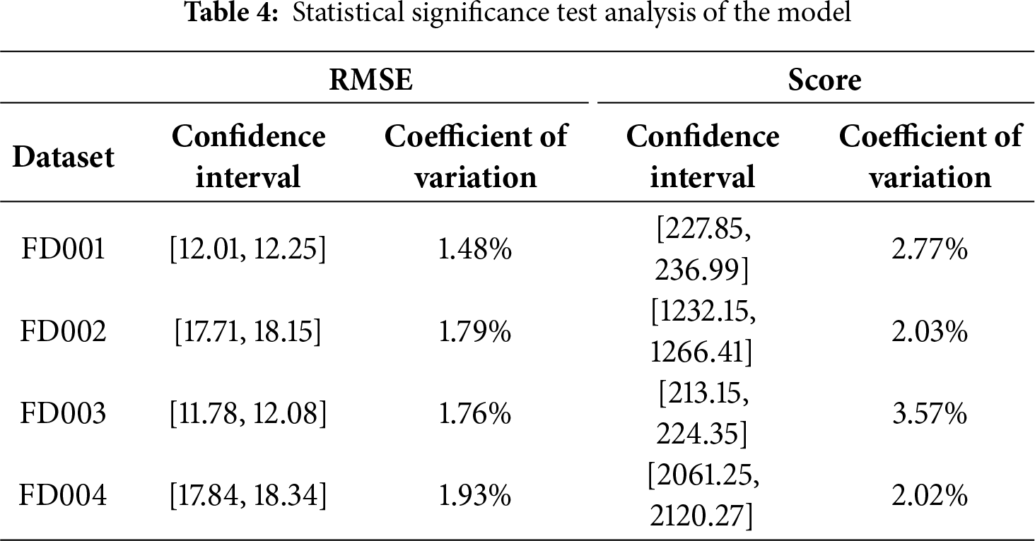
To verify the statistical significance and robustness of the proposed method, we conducted systematic replicate experiments. For the four subsets of the C-MAPSS dataset, the model was independently run under identical experimental settings using 10 different random seeds (42, 123, 456, 789, 999, 111, 222, 333, 444, 555). Each experiment included a complete workflow of data preprocessing, model training, and evaluation to ensure strict consistency of experimental conditions. The significance test analysis of the proposed method is presented in Table 4, which includes the mean, coefficient of variation, and 95% confidence interval of the RMSE and Score metrics, providing a comprehensive evaluation of the model’s robustness across different datasets.

To further analyze the RUL prediction accuracy on the C-MAPSS dataset, visualizations of the prediction results for all four subsets are provided in Figs. 7 and 8. Fig. 7 illustrates the overall prediction performance across all test engines within each subset, while Fig. 8 depicts the results for individual engines. As shown in the subplots of Fig. 7, a noticeable deviation between the predicted and actual RUL values is observed when the true RUL is high. However, as the true RUL approaches zero, the predicted and actual curves converge, demonstrating improved alignment and smoother fitting. The overall trends captured in Fig. 8 reveal that the predicted curves consistently follow the true RUL trajectories, particularly during the critical degradation phase of the engines. This indicates the model’s capability to accurately reflect the gradual decline in RUL and capture the underlying degradation trends. These results visually underscore the robustness of the model in scenarios involving rapid health deterioration, highlighting its practical suitability for providing timely and accurate early warnings in industrial fault prediction systems.

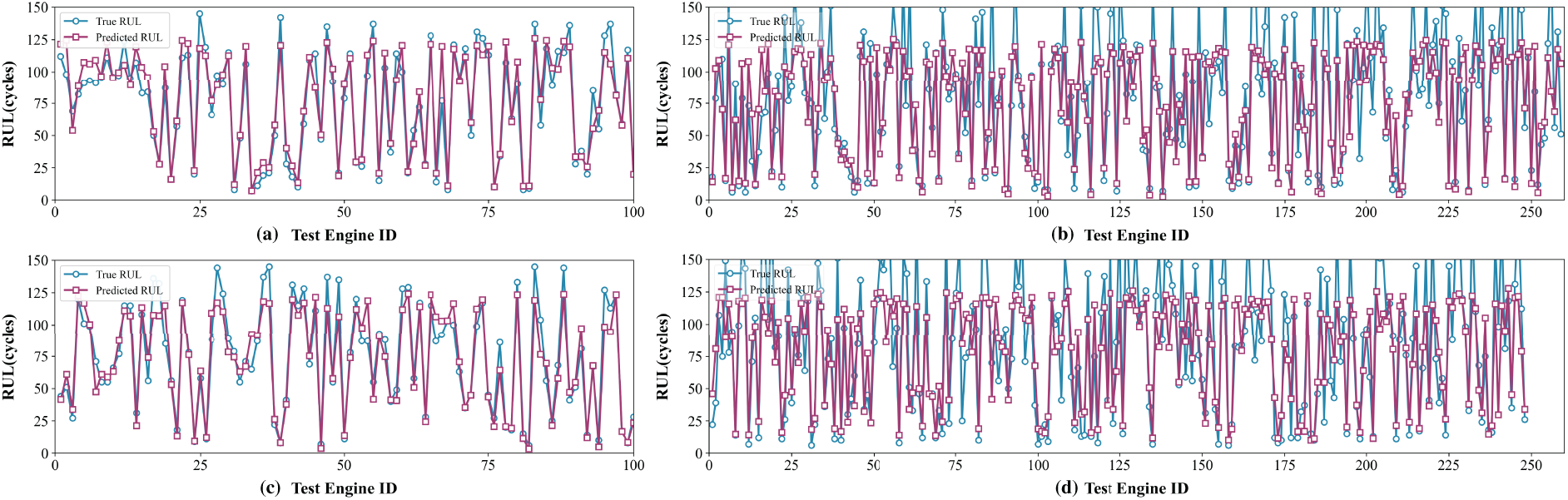
Figure 7: RUL prediction results for all engines in FD001 (a), FD002 (b), FD003 (c), and FD004 (d)

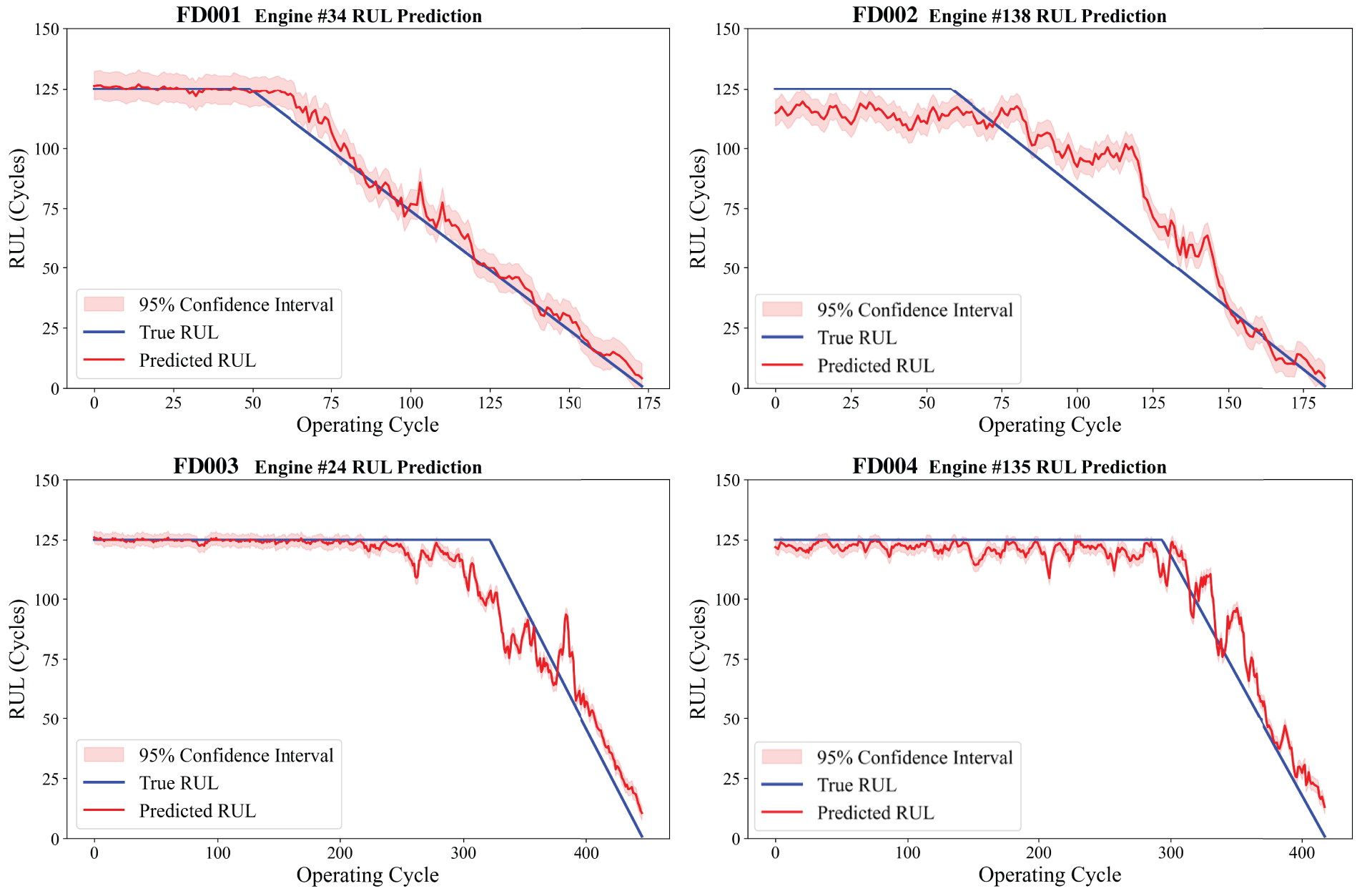
Figure 8: RUL prediction results for a representative individual engine from each subset

In addition, the probability density prediction distribution for individual engine lifetimes within four subsets was visualized, as shown in Figs. 9–12. The results demonstrate that the proposed method achieves accurate RUL predictions under various operating conditions and scenarios, with prediction errors consistently lower than those of the traditional LSTM model. The probability density curves exhibit a Gaussian distribution, and the predicted RUL means show minimal deviation from the actual values. From a maintenance perspective, the shape and spread of these distributions are highly informative. For instance, in Fig. 10a,b, the narrow and sharp distribution indicates high prediction confidence, suggesting that maintenance can be scheduled with high certainty around the mean RUL. The proposed framework not only maintains a low mean squared error but also generates probability distribution curves, which are unavailable through traditional method. This advancement shifts the prediction paradigm from “point estimation” to “risk quantification,” highlighting the value of probabilistic prediction in maintenance decision-making.

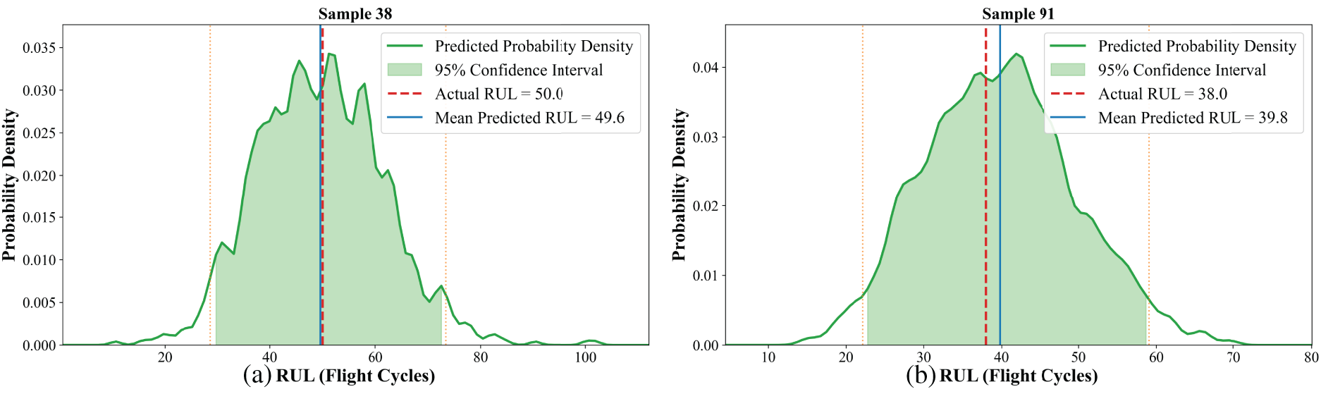
Figure 9: Probability density prediction distribution of sample 38 (a) and sample 91 (b) in the FD001 subset

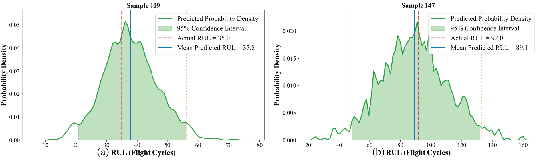
Figure 10: Probability density prediction distribution of sample 109 (a) and sample 147 (b) in the FD002 subset

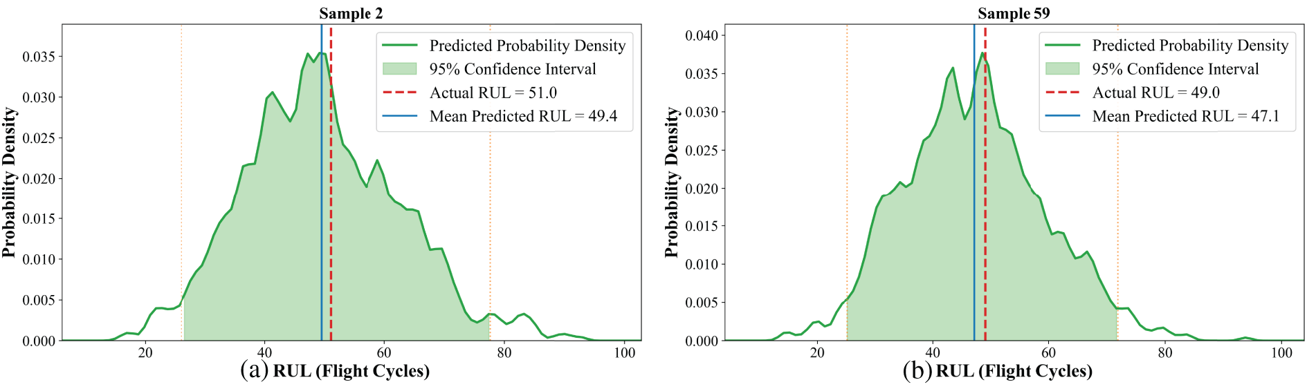
Figure 11: Probability density prediction distribution of sample 2 (a) and sample 59 (b) in the FD003 subset

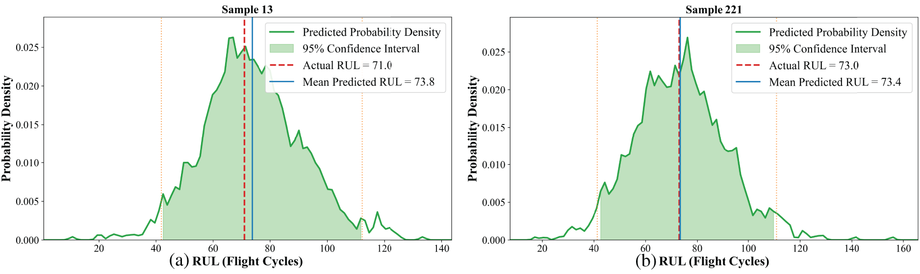
Figure 12: Probability density prediction distribution of 13 (a) and sample 221 (b) in the FD004 subset

The model exhibits two main types of RUL prediction bias: (1) slight overestimation during early-to-mid operation due to weak degradation signals being masked by noise. Although the attention mechanism aims to focus on key information, the model struggles to extract strongly predictive early degradation patterns from complex multi-sensor signals when degradation features are not yet prominent. (2) occasional significant underestimation near failure end for units with abrupt performance drops, likely due to insufficient training data on such rapid degradation patterns. This is likely because training data contains relatively few examples of rapid failure, preventing the model from adequately learning the dynamics of fast degradation.

4.5 Ablation Study

To quantitatively evaluate the individual contribution of each key component in the proposed framework—namely the Attention mechanism, Residual Connections, and the KDE-based probabilistic framework, a comprehensive ablation study was conducted. The objective is to isolate the impact of these components on the model’s overall prediction performance and its uncertainty quantification capability.

The ablation experiments were performed on four subsets under identical experimental settings (e.g., hyperparameters, training-testing split) as the full model. We designed three model variants for comparison: Variant A (w/o Attention), Variant B (w/o Residual), and Variant C (w/o KDE). The results of the ablation study are summarized in Table 5.

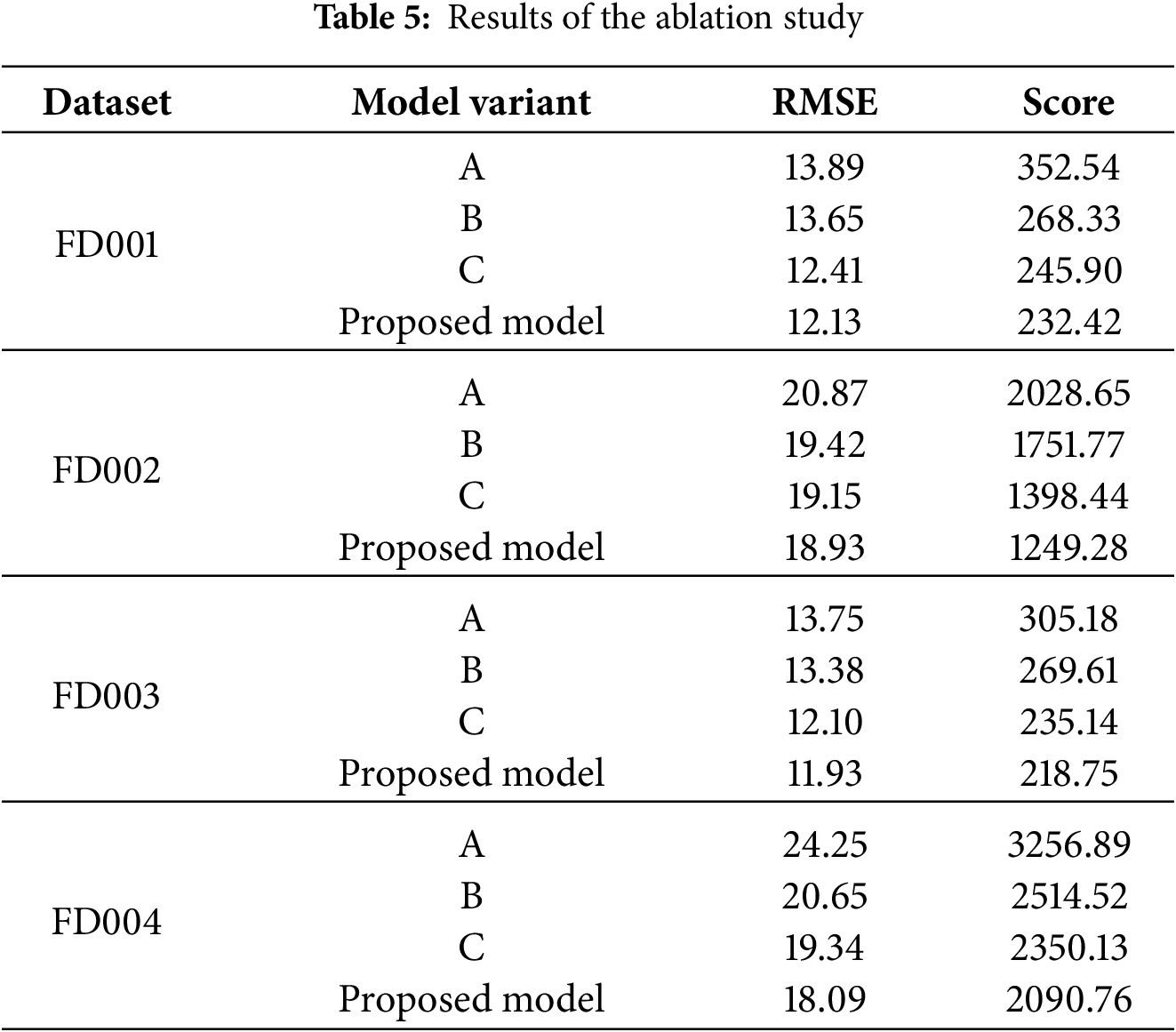
In conclusion, the attention mechanism enables temporal feature selection, residual connections ensure stable training of deep networks, and the KDE framework provides essential uncertainty quantification for risk-conscious decision-making. Their synergistic integration in the full model is justified by its superior and robust performance across all evaluation scenarios.

5  Conclusion

This study has successfully established an integrated deep learning framework for the probabilistic prediction of RUL, effectively addressing key challenges in processing noisy sensor data and quantifying predictive uncertainty. This work provides a complete probabilistic RUL prediction solution spanning from data processing to decision-making. The value of this solution lies in the fact that the output probability distribution can be directly applied to risk assessment and maintenance strategy optimization, thereby offering a new technical approach for health management of complex mechanical systems. The main conclusions are as follows:

The proposed fusion neural network significantly enhances a superior capability in modeling complex, nonlinear degradation patterns from multi-sensor time-series data, outperforming conventional models and achieving higher prediction accuracy on the benchmark C-MAPSS dataset.

A well-balanced trade-off among model capacity, training efficiency, and generalization ability is achieved. The framework strikes a careful balance between model capacity and generalization through the synergistic use of residual connections and stochastic regularization, ensuring stable training and robust performance.

The incorporation of KDE enhances the robustness of RUL predictions and enables uncertainty quantification. The framework improves the accuracy of interval predictions, thereby offering more reliable decision support for equipment health management.

Although the proposed framework demonstrates superior performance in RUL probability prediction, several limitations remain. The current work primarily relies on homogeneous sensor sequences and has not yet explored the deep integration of multi-modal sensor information. Furthermore, the model’s cross-equipment transfer learning capability requires validation, and a dynamic updating mechanism for online streaming PHM systems has not been implemented.

Future research will focus on extending the framework to incorporate multi-source heterogeneous information fusion, developing efficient transfer learning strategies, and constructing a dynamic prediction framework capable of online adaptive learning, thereby further enhancing the model’s practicality and generalization in complex industrial scenarios.

Acknowledgement: Not applicable.

Funding Statement: This research was funded by scientific research projects under Grant JY2024B011.

Author Contributions: The authors confirm contribution to the paper as follows: Conceptualization, Bo Zhu, Zhonghua Cheng; methodology, Shuai Yue; software, Enzhi Dong; validation, Kexin Jiang; formal analysis, Bo Zhu; investigation, Enzhi Dong, Shuai Yue, Chiming Guo; resources, Shuai Yue; data curation, Shuai Yue, Chiming Guo; writing—original draft preparation, Bo Zhu; writing—review and editing, Enzhi Dong, Kexin Jiang, Zhonghua Cheng; visualization, Kexin Jiang; supervision, Zhonghua Cheng, Chiming Guo; project administration, Zhonghua Cheng, Chiming Guo. All authors reviewed the results and approved the final version of the manuscript.

Availability of Data and Materials: Data available on request from the authors. The data that support the findings of this study are available from the corresponding author, Zhonghua Cheng, upon reasonable request.

Ethics Approval: Not applicable.

Conflicts of Interest: The authors declare no conflicts of interest to report regarding the present study.

References

1. Qiu LJ, Wu MH. PHM technology framework and its key technologies review. Foreign Electron Meas Technol. 2018;37(2):10–5. (In Chinese). doi:10.19652/j.cnki.femt.1700638. [Google Scholar] [CrossRef]

2. Kong JZ, Liu J, Zhu JZ, Zhang X, Tsui KL, Peng ZK, et al. Review on lithium-ion battery PHM from the perspective of key PHM steps. Chin J Mech Eng. 2024;37(4):14–35. doi:10.1186/s10033-024-01055-z. [Google Scholar] [CrossRef]

3. Jin RB, Chen ZH, Wu KY, Wu M, Li XL, Yan RQ. Bi-LSTM-based two-stream network for machine remaining useful life prediction. IEEE Trans Instrum Meas. 2022;71:3511110. doi:10.1109/TIM.2022.3167778. [Google Scholar] [CrossRef]

4. Song JW, Park YI, Hong JJ, Kim SG, Kang SJ. Attention-based bidirectional LSTM-CNN model for remaining useful life estimation. In: 2021 IEEE International Symposium on Circuits and Systems (ISCAS); 2021 May 22–28; Virtual. p. 1–5. doi: 10.1109/ISCAS51556.2021.9401572. [Google Scholar] [CrossRef]

5. Cai S, Zhang JW, Li C, He ZQ, Wang ZM. A RUL prediction method of rolling bearings based on degradation detection and deep BiLSTM. Electron Res Arch. 2024;32(5):3145–61. doi:10.3934/era.2024144. [Google Scholar] [CrossRef]

6. Guo XF, Wang KZ, Yao S, Fu GJ, Ning Y. RUL prediction of lithium ion battery based on CEEMDAN-CNN BiLSTM model. Energy Rep. 2023;9(1):1299–306. doi:10.1016/j.egyr.2023.05.121. [Google Scholar] [CrossRef]

7. Raouf I, Kumar P, Khalid S, Kim HS. Comprehensive analysis of current developments, challenges, and opportunities for the health assessment of smart factory. Int J Precis Eng Manuf-Green Technol. 2025;12(4):1321–38. doi:10.1007/s40684-025-00694-4. [Google Scholar] [CrossRef]

8. Kumar P, Khalid S, Kim HS. Prognostics and health management of rotating machinery of industrial robot with deep learning applications—a review. Math. 2023;11(13):3008. doi:10.3390/math11133008. [Google Scholar] [CrossRef]

9. Raouf I, Lee H, Kim HS. Mechanical fault detection based on machine learning for robotic RV reducer using electrical current signature analysis: a data-driven approach. J Comput Des Eng. 2022;9(2):417–33. doi:10.1093/jcde/qwac015. [Google Scholar] [CrossRef]

10. Raouf I, Kumar P, Kim HS. Deep learning-based fault diagnosis of servo motor bearing using the attention-guided feature aggregation network. Expert Syst Appl. 2024;258(4):125137. doi:10.1016/j.eswa.2024.125137. [Google Scholar] [CrossRef]

11. Ma MY. Application of deep learning in fault diagnosis and life prediction of rolling bearings [dissertation]. Nanjing, China: Nanjing University of Information Science and Technology; 2024. doi: 10.27248/d.cnki.gnjqc.2024.000262. [Google Scholar] [CrossRef]

12. Zhang ZZ. Research on remaining useful life prediction methods for mechanical equipment based on deep learning [dissertation]. Jinan, China: Shandong University; 2024. doi: 10.27272/d.cnki.gshdu.2024.000382. [Google Scholar] [CrossRef]

13. Zha WT, Ye YH. An aero-engine remaining useful life prediction model based on feature selection and the improved TCN. Franklin Open. 2024;6(5):100083. doi:10.1016/j.fraope.2024.100083. [Google Scholar] [CrossRef]

14. Chen FD, Yu Y, Li YJ. An aero-engine remaining useful life prediction model based on clustering analysis and the improved GRU-TCN. Meas Sci Technol. 2025;36(1):016001. doi:10.1088/1361-6501/ad825a. [Google Scholar] [CrossRef]

15. Zhu B, Dong E, Cheng Z, Zhan X, Jiang K, Wang R. An integrated approach to condition-based maintenance decision-making of planetary gearboxes: combining temporal convolutional network auto encoders with wiener process. Comput Mater Contin. 2025;86(1):1–26. doi:10.32604/cmc.2025.069194. [Google Scholar] [CrossRef]

16. He D, Zhao J, Jin Z, Huang C, Yi C, Wu J. DCAGGCN: a novel method for remaining useful life prediction of bearings. Reliab Eng Syst Saf. 2025;260(9):110978. doi:10.1016/j.ress.2025.110978. [Google Scholar] [CrossRef]

17. Liao Y, Zhang L, Liu C. Uncertainty prediction of remaining useful life using long short-term memory network based on bootstrap method. In: Proceedings of the 2018 IEEE International Conference on Prognostics and Health Management (ICPHM); 2018 Jun 11–13; Seattle, WA, USA. p. 1–8. doi: 10.1109/ICPHM.2018.8448804. [Google Scholar] [CrossRef]

18. Xiang S, Qin Y, Luo J, Pu H, Tang B. Multicellular LSTM-based deep learning model for aero-engine remaining useful life prediction. Reliab Eng Syst Saf. 2021;216:107927. doi:10.1016/j.ress.2021.107927. [Google Scholar] [CrossRef]

19. Chen X, Tian Z. A novel method for identifying sudden degradation changes in remaining useful life prediction for bearing. Expert Syst Appl. 2025;278(3):127315. doi:10.1016/j.eswa.2025.127315. [Google Scholar] [CrossRef]

20. Yu W, Kim IY, Mechefske C. An improved similarity-based prognostic algorithm for RUL estimation using an RNN autoencoder scheme. Reliab Eng Syst Saf. 2020;199:106926. doi:10.1016/j.ress.2020.106926. [Google Scholar] [CrossRef]

21. Zhang J, Jiang Y, Wu S, Li X, Luo H, Yin S. Prediction of remaining useful life based on bidirectional gated recurrent unit with temporal self-attention mechanism. Reliab Eng Syst Saf. 2022;221(4):108297. doi:10.1016/j.ress.2021.108297. [Google Scholar] [CrossRef]

22. Al-Dulaimi A, Zabihi S, Asif A, Mohammadi A. A multimodal and hybrid deep neural network model for remaining useful life estimation. Comput Ind. 2019;108:186–96. doi:10.1016/j.compind.2019.02.004. [Google Scholar] [CrossRef]

23. Chen Z, Wu M, Zhao R, Guretno F, Yan R, Li X. Machine remaining useful life prediction via an attention-based deep learning approach. IEEE Trans Ind Electron. 2021;68(3):2521–31. doi:10.1109/TIE.2020.2972443. [Google Scholar] [CrossRef]

24. Shan Y, Xiao L, Fang X. Predicting the remaining useful life of aircraft engines using spatial and temporal attention mechanisms. IEEE Trans Instrum Meas. 2025;74:1–14. doi:10.1109/TIM.2025.3545540. [Google Scholar] [CrossRef]

25. Gao Z, Jiang W, Wu J, Dai T. Multiscale spatiotemporal attention network for remaining useful life prediction of mechanical systems. IEEE Sens J. 2025;25(4):6825–35. doi:10.1109/JSEN.2024.3523176. [Google Scholar] [CrossRef]

26. Han B, Yin P, Zhang Z, Wang J, Bao H, Song L, et al. Remaining useful life prediction of turbofan engines based on dual attention mechanism guided parallel CNN-LSTM. Meas Sci Technol. 2025;36(1):016160. doi:10.1088/1361-6501/ad8946. [Google Scholar] [CrossRef]

27. Zhang W, Zhang X, Yan X, Xu Y, Cai J. Remaining useful life prediction of motor bearings based on slow feature analysis-assisted attention mechanism and dual-LSTM networks. Struct Health Monit. 2025;1(1):97. doi:10.1177/14759217251324103. [Google Scholar] [CrossRef]

28. Liu M, Zheng D, Gou P, Zhang J, Lai Z, Chen D, et al. A two-phase equipment remaining useful life prediction model with sequence-feature attention mechanism. IEEE Trans Instrum Meas. 2025;74(4):1–14. doi:10.1109/TIM.2025.3576953. [Google Scholar] [CrossRef]

29. Bahdanau D, Cho K, Bengio Y. Neural machine translation by jointly learning to align and translate. arXiv:1409.0473. 2014. doi:10.48550/arXiv.1409.0473. [Google Scholar] [CrossRef]

30. Le Folgoc L, Baltatzis V, Desai S, Devaraj A, Ellis S, Manzanera OEM, et al. Is MC dropout Bayesian? arXiv:2110.04286. 2021. doi: 10.48550/arXiv.2110.04286. [Google Scholar] [CrossRef]

31. Gal Y, Ghahramani Z. Dropout as a Bayesian approximation: representing model uncertainty in deep learning. arXiv:1506.02142. 2015. doi: 10.48550/arXiv.1506.02142. [Google Scholar] [CrossRef]

32. Saxena A, Goebel K, Simon D, Eklund N. Damage propagation modeling for aircraft engine run-to-failure simulation. In: Proceedings of the International Conference on Prognostics and Health Management; 2008 Oct 6–9; Denver, CO, USA. Piscataway, NJ, USA: IEEE; 2008. p. 1–9. doi:10.1109/PHM.2008.4711414. [Google Scholar] [CrossRef]