
 Submit a Paper
 Propose a Special lssue
 Open Access
ARTICLE
Actor–Critic Trajectory Controller with Optimal Design for Nonlinear Robotic Systems
1 Graduate Institute of Automation Technology, National Taipei University of Technology, Taipei, 10608, Taiwan
2 Computer Science and Information Engineering, National Taipei University of Technology, Taipei, 10608, Taiwan
* Corresponding Author: Nien-Tsu Hu. Email:
Computers, Materials & Continua 2026, 87(1), 83 https://doi.org/10.32604/cmc.2025.074993
Received 22 October 2025; Accepted 18 December 2025; Issue published 10 February 2026
 View Full Text
 Download PDF
Abstract
Trajectory tracking for nonlinear robotic systems remains a fundamental yet challenging problem in control engineering, particularly when both precision and efficiency must be ensured. Conventional control methods are often effective for stabilization but may not directly optimize long-term performance. To address this limitation, this study develops an integrated framework that combines optimal control principles with reinforcement learning for a single-link robotic manipulator. The proposed scheme adopts an actor–critic structure, where the critic network approximates the value function associated with the Hamilton–Jacobi–Bellman equation, and the actor network generates near-optimal control signals in real time. This dual adaptation enables the controller to refine its policy online without explicit system knowledge. Stability of the closed-loop system is analyzed through Lyapunov theory, ensuring boundedness of the tracking error. Numerical simulations on the single-link manipulator demonstrate that the method achieves accurate trajectory following while maintaining low control effort. The results further show that the actor–critic learning mechanism accelerates convergence of the control policy compared with conventional optimization-based strategies. This work highlights the potential of reinforcement learning integrated with optimal control for robotic manipulators and provides a foundation for future extensions to more complex multi-degree-of-freedom systems. The proposed controller is further validated in a physics-based virtual Gazebo environment, demonstrating stable adaptation and real-time feasibility.Keywords
In recent years, intelligent and optimized methodologies for nonlinear system control have drawn significant attention. Owing to the complexity of nonlinear dynamics, traditional linear control approaches are often inadequate in practical applications. To address unknown dynamics and uncertainties, artificial neural networks (ANNs), especially radial basis function neural networks (RBFNNs), have been widely used for nonlinear system modelling and controller design. With Lyapunov-based adaptation schemes, such RBFNN-based controllers can guarantee that all closed-loop signals are semi-globally uniformly ultimately bounded (SGUUB) [1].
On the other hand, the mathematical foundation of optimal control is based on the Hamilton–Jacobi–Bellman (HJB) equation, which is generally intractable for nonlinear systems. Approximation methods such as Galerkin schemes have been developed to provide feasible solutions, laying the groundwork for the integration of adaptive dynamic programming (ADP) and reinforcement learning (RL) into nonlinear control [2]. From a theoretical standpoint, the foundations of nonlinear analysis and stability are systematically presented in Khalil’s Nonlinear Systems, which covers Lyapunov stability, backstepping, and input–output stability [3]. Similarly, the comprehensive framework of optimal control, extending from linear quadratic regulation (LQR) to nonlinear HJB approaches, is well established in Lewis’s Optimal Control [4].
More recently, advanced RL-based methods have been introduced for robotic systems subject to complex constraints. For instance, Peng et al. developed an event-sampled critic learning strategy to solve the optimal tracking control problem of motion-constrained robot manipulators, reducing computational burden while ensuring stability [5]. Cheng and Dong proposed a single-critic neural network approach for robotic manipulators with input saturation and disturbances, with stability guaranteed through Lyapunov theory [6]. Hu et al. further extended actor–critic network designs to handle manipulators with dynamic disturbances, ensuring SGUUB stability and accurate trajectory tracking [7].
In addition, Wen et al. proposed optimized adaptive tracking and backstepping frameworks that integrate actor–critic RL into nonlinear control. In these works, both virtual and actual control inputs are designed as optimal solutions at each recursive step, and the resulting controllers simultaneously achieve trajectory tracking and performance optimization [8,9]. In the broader context of multi-agent systems (MASs), Wen et al. further introduced an identifier–actor–critic algorithm based on fuzzy logic systems for MASs with unknown nonlinear dynamics, addressing state coupling and ensuring stability under Lyapunov analysis [10]. These representative studies highlight how filtered or composite errors can be exploited to structure the optimal tracking problem in both single-system and multi-agent settings.
Beyond these developments, many tracking designs employ the reference error to streamline stability analysis and shape tracking dynamics [11]. For transient and steady-state guarantees, prescribed-performance control (PPC) provides Lyapunov-based performance envelopes that accommodate uncertainties and actuator limitations in robotic manipulators; recent works further strengthen PPC with Barrier Lyapunov Function (BLF)-based designs, assigned/appointed settling time, and neural adaptations [12–14]. On the optimal-learning side, actor–critic reinforcement learning has been applied to robotic manipulators to enhance practical tracking performance with stability-oriented designs, and RL-based controllers have also been developed for nonlinear syst ems such as single-link manipulators [15,16]. Moreover, model-based actor–critic learning has been exploited for robotic impedance control in complex interactive environments, where the actor–critic framework is used to learn impedance behavior for safe and efficient robot–environment interaction [17].
In parallel, integral and off-policy reinforcement learning techniques have been investigated to address optimal tracking under disturbances, input constraints, and model uncertainty. For perturbed discrete-time systems, H∞ tracking control frameworks based on On/Off policy Q-learning have been proposed, where model-free Q-learning algorithms are shown to guarantee convergence of the learned policy in the presence of external disturbances [18]. For perturbed bilateral teleoperators with variable time delay, nonlinear RISE-based integral RL algorithms have been developed by combining robust integral action with actor–critic structures to achieve both optimal performance and coordination tracking [19]. Off-policy integral RL-based optimal tracking schemes have also been proposed for nonzero-sum game systems with unknown dynamics, further relaxing model requirements while maintaining stability and disturbance attenuation [20].
Together, these contributions indicate that the integration of RBFNNs, Lyapunov stability analysis, HJB approximations, and actor–critic reinforcement learning provides an effective pathway for solving nonlinear optimal tracking problems. At the same time, most existing RL-based optimal tracking schemes still exhibit several limitations: many require partial model knowledge or rely on Persistent of Excitation (PE)-type excitation conditions to guarantee convergence of the actor–critic networks, and the transient dynamics are usually determined implicitly by Lyapunov designs rather than by an explicitly tunable reference-error structure. In addition, the interaction between optimal cost design, actuator constraints, and reference-error shaping has not been fully explored in the context of nonlinear robotic systems.
To clarify how the proposed scheme is tailored to address the above gaps, we explicitly match each limitation with a corresponding design element of our method.
(i) Reliance on partial model knowledge: many RL/HJB/ADP controllers still require certain model components for policy/value formulation and stability analysis; our approach integrates an online actor–critic structure with RBFNN approximation to reduce dependence on precise model parameters while retaining Lyapunov-based stability analysis (see Sections 3 and 4).
(ii) Persistence of excitation (PE) requirements: theoretical convergence of adaptive/learning laws typically relies on PE; we adopt a standard PE condition for weight convergence analysis and provide implementation-oriented discussions/experiments to illustrate stable learning under practical excitation levels (Assumption 2 in Section 3.2; results in Sections 5 and 6).
(iii) Implicit transient tuning: transient behavior is often tuned implicitly through multiple gains without a clear performance knob; we introduce a structured reference-error design with an explicit gain to shape tracking dynamics in a transparent manner, while preserving the Lyapunov proof (see Sections 2 and 4; parameter study in Section 5).
(iv) Lack of a structured reference-error mechanism in optimal learning designs: by embedding the reference-error into the learning/control formulation, the proposed method establishes a one-to-one link between tracking-dynamics shaping and optimal-learning updates, which is validated in both numerical simulations and physics-based environments (see Sections 2, 3, 5 and 6).
Motivated by these developments and limitations, this work proposes a reinforcement learning–based optimal tracking control framework for robotic manipulators, with a particular focus on trajectory tracking under nonlinear dynamics. The key novelty of this work lies in augmenting the actor–critic optimal control framework with a tunable reference error structure, enabling direct adjustment of convergence speed while preserving Lyapunov stability guarantees and real-time implementability in both numerical and physics-based environments.
Contributions of this work are summarized as follows:
1. A structured reference-error formulation that explicitly shapes tracking transients with a tunable gain.
2. A Lyapunov-stability-oriented actor–critic learning design with online approximation.
3. Comparative studies and validations in both numerical simulations and physics-based environments.
The single-link robotic manipulator is widely used as a benchmark system to evaluate nonlinear control methods. Its dynamic equation can be expressed as
where
Following the definition of the manipulator dynamics in Eq. (1), the tracking error with respect to a desired trajectory
To enforce convergence of the tracking error, reference error is defined as
where
Substituting Eq. (1) into the above, the closed-loop error channel can be rearranged as
where
and the augmented state is given by
Introducing the auxiliary input
the error dynamics reduce to
Combining with Eq. (3), the augmented system can be expressed in compact form as
Assumption 1: The system dynamics
Remark 1: Although Eq. (9) is written in a compact state-space form that is linear in the error state vector
To measure tracking performance and input usage, we introduce the performance index in terms of a running-cost surrogate:
with the running cost
where
Definition 1: A control strategy
Here,
According to optimal control theory, the Hamilton–Jacobi–Bellman (HJB) equation for this problem can be written as
where
By applying the optimality condition
Thus, the solution to the control problem requires finding the optimal policy
3 Optimal Control with Reinforcement Learning
3.1 Radial Basis Function Neural Network (RBFNN) Approximation
To facilitate the construction of the optimal tracking control law, the optimal performance function
where
Since neural networks have the capability to approximate continuous functions with arbitrary accuracy on a compact domain, the residual term
where
By substituting the approximation Eq. (15) into the decomposition Eq. (14), the gradient of
According to the optimal control policy derived in Eq. (13), the optimal input can be rewritten as
By substituting Eqs. (16) and (17) into Eq. (12), the following result can be obtained:
where
Remark 2: The number of radial basis function (RBF) nodes has a direct impact on both the approximation capability and the closed-loop performance. In this work, Gaussian RBFNNs are adopted for both the critic and actor, and the centers are uniformly distributed over the estimated reachable region of the state vector. Preliminary simulations with different node numbers (e.g., 25, 36, and 49) indicate that 36 nodes provide a good trade-off between approximation accuracy and online computational complexity; therefore, this configuration is used in the final simulations.
From the viewpoint of function approximation, too few basis functions lead to insufficient representation power and large residual errors, which may slow down learning and degrade tracking performance. On the other hand, using too many RBF nodes increases the network dimension and may cause overfitting and high-variance responses. In our simulations, when the number of nodes is excessively large, the learned control policy tends to exhibit sharper variations and high-frequency oscillations, resulting in “spiky” tracking trajectories and more aggressive control actions. A similar trade-off between approximation accuracy and model complexity has been reported in adaptive neural network control of robot manipulators, where an optimal number of hidden nodes is sought to avoid both under-fitting and over-fitting of the unknown dynamics [21].
3.2 Actor–Critic Implementation
In practice, the ideal weight vector
The critic network approximates the performance index as
where
Accordingly, the actor generates the control input using both the critic information and its own adaptive weights:
where
Therefore, the actor–critic pair collaborates such that the critic approximates the gradient
The Bellman residual is defined in terms of the Hamiltonian as
since the Hamiltonian at the optimal policy
expanding Eq. (22), the Bellman residual can be written explicitly as
to minimize the Bellman residual error
is introduced. For stability, it is required that
The critic weight updating rule is obtained by applying a normalized negative gradient descent:
where
The actor weight adaptation rule is derived from stability analysis to ensure that the optimized control input remains stable. The actor weights are updated according to
where
Assumption 2: In this work, we adopt the standard concept of persistence of excitation (PE) as a requirement for ensuring sufficient richness in the regressor signal. Let
where
In this section, the stability of the closed-loop system is analyzed using a Lyapunov-based method. Consider the following Lyapunov candidate function:
where
The time derivative of
Applying Eqs. (20), (25) and (26) to Eq. (28), the following equation can be formulated as:
Based on
According to Young’s and Cauchy inequalities [10], we obtain the results below:
Substituting into (29), the following equation follows:
Based on (18), we obtain the equation shown below:
By inserting (35) into (34), the following result is obtained:
Using the fact that:
Eq. (36) is obtained:
Substituting the facts that
Substituting Eqs. (39) and (40) into Eq. (38) yields:
where
Using Young’s and Cauchy inequalities, we obtain the bounds shown below:
By substituting the inequalities in Eqs. (42) and (43) into Eq. (41), we obtain:
Let
where
equivalently,
where
Lemma 1 [1]: Consider a scalar function
By Lemma 1, Eq. (47) can be obtained:
Result. Inequality Eq. (32) implies that the errors
Finally, our proposed actor–critic trajectory controller with optimal design for nonlinear robotic systems is shown in Fig. 1.
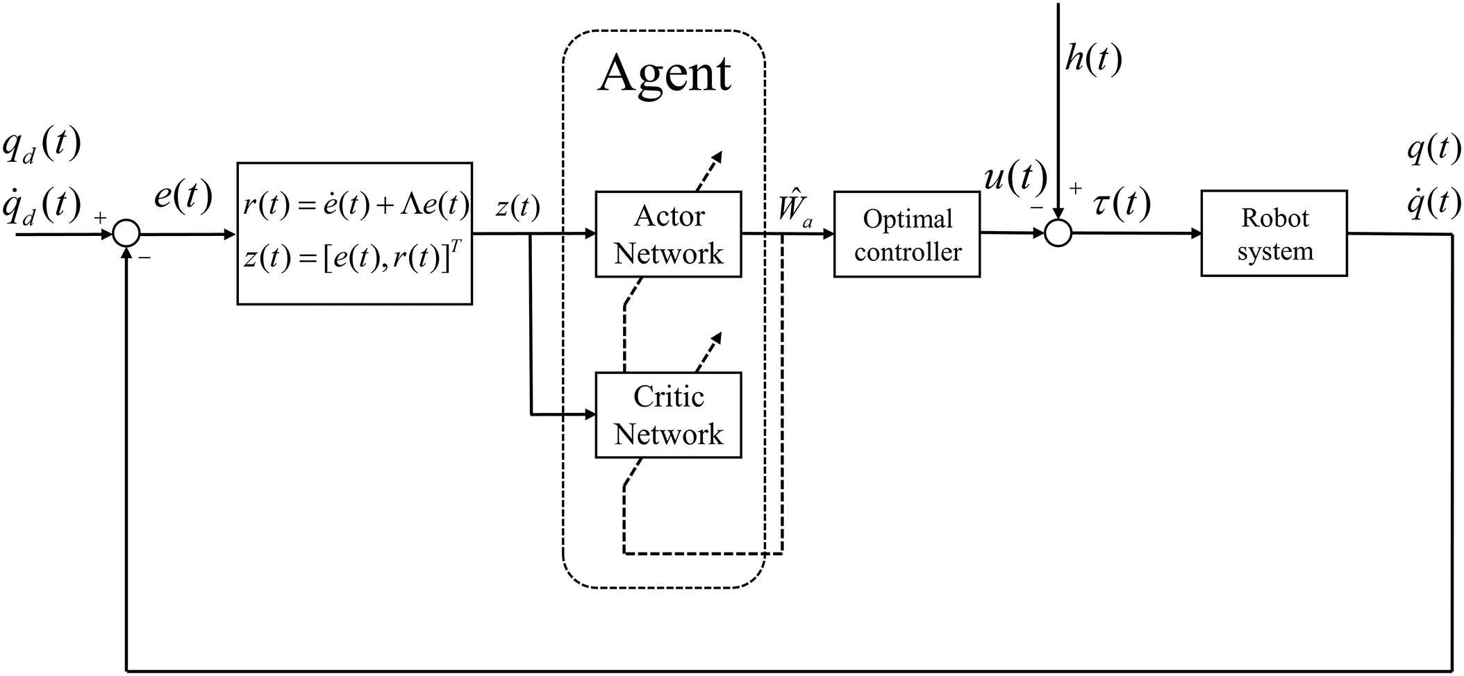
Figure 1: Our proposed actor–critic trajectory controller with optimal design for nonlinear robotic systems
5 Numerical Simulation Results
The effectiveness of the control scheme is assessed on a single-link robotic manipulator governed by Eq. (1). The system parameters follow Section 2.1 and are fixed as
For the neural network approximation, RBFNN with 36 units is adopted. The basis vector takes the form
with each Gaussian basis function given by
where
The control design parameters are selected as
Two controllers are compared under identical conditions. The first follows the method in [8], which uses the tracking error
For the baseline controller based on [8], we reimplemented the algorithm under exactly the same settings as those described above for the proposed method. In particular, both controllers use the same single-link manipulator dynamics in Section 2, the same desired trajectory, the same parameters, and the same RBFNN structure (number of nodes, centers and widths) for the critic and actor. Moreover, the critic and actor learning rates and, the initial weight vectors, and the initial state of the system are chosen to be identical for the baseline and the proposed controller. Therefore, the performance differences observed in this subsection mainly originate from the structural modification introduced in this work, rather than from arbitrary retuning of the underlying parameters.
Fig. 2 presents position and velocity tracking results. The method proposed in this paper produces markedly faster transients; increasing
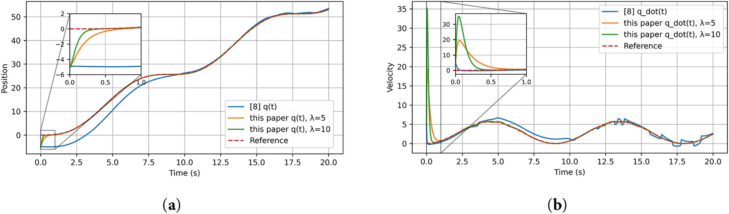
Figure 2: Position and velocity tracking of the single-link manipulator: (a) position comparison between the method in [8] and the proposed method; (b) velocity comparison between the method in [8] and the proposed method. All curves are generated from our own simulations based on the controller structure reported in [8]

Figure 3: Tracking errors of the single-link manipulator: (a) position error; (b) velocity error
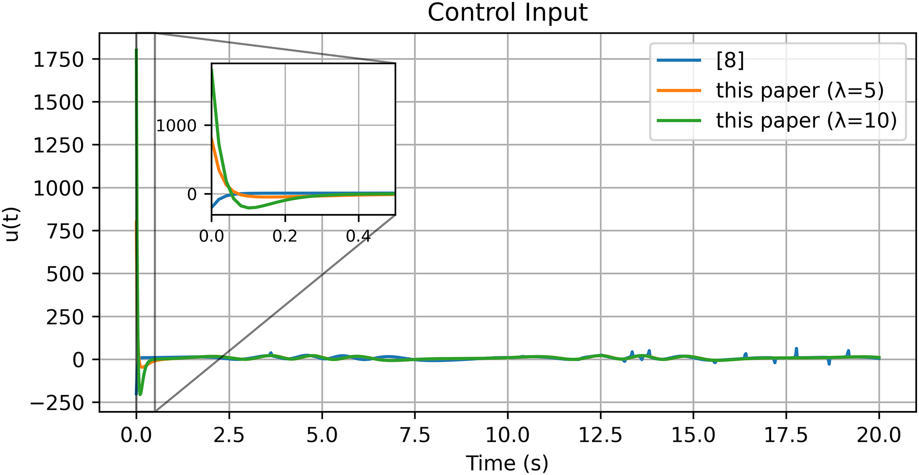
Figure 4: Control input
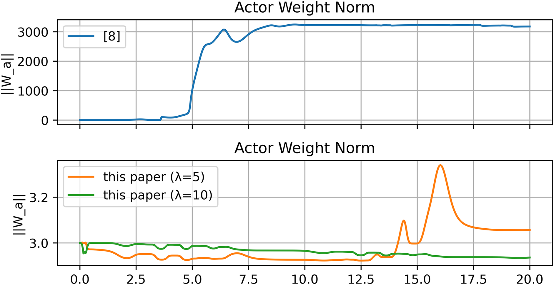
Figure 5: Norm of actor Neural Network (NN) weights
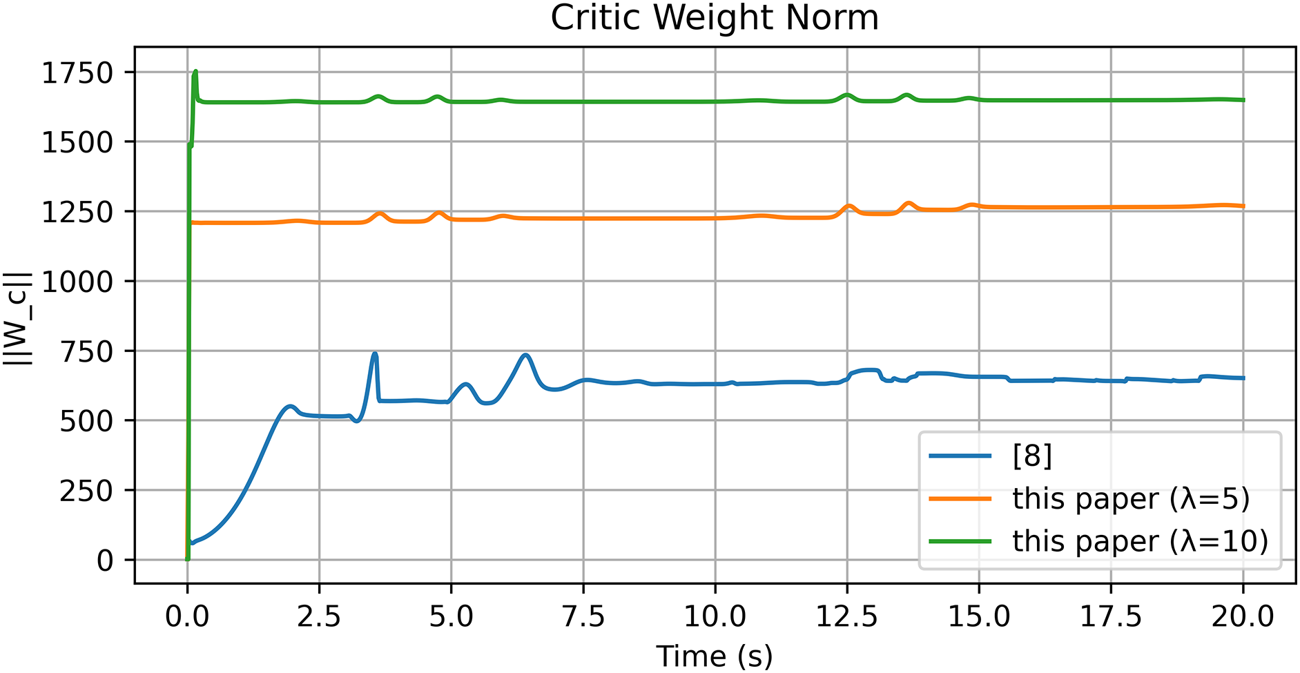
Figure 6: Norm of critic NN weights
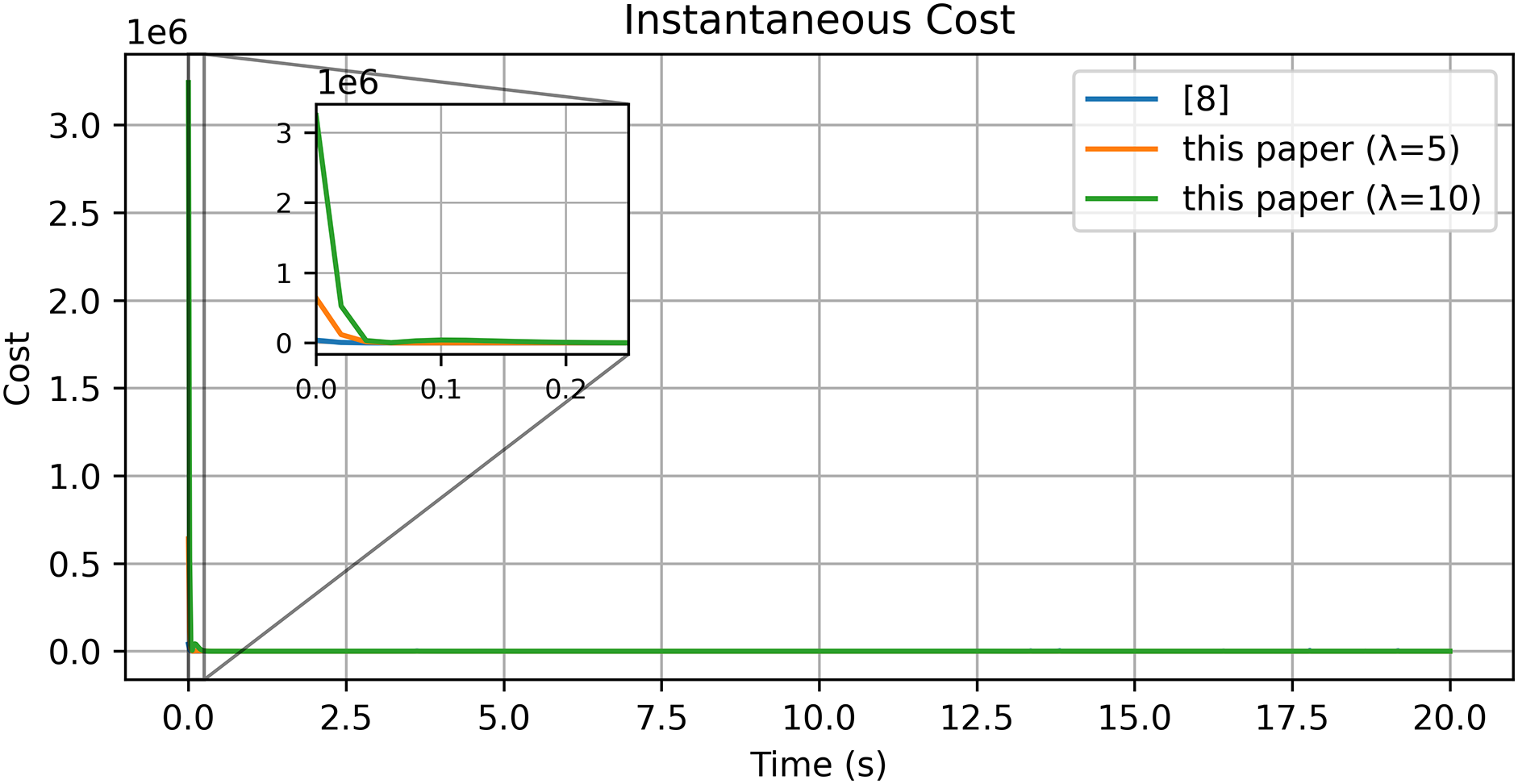
Figure 7: Cost function
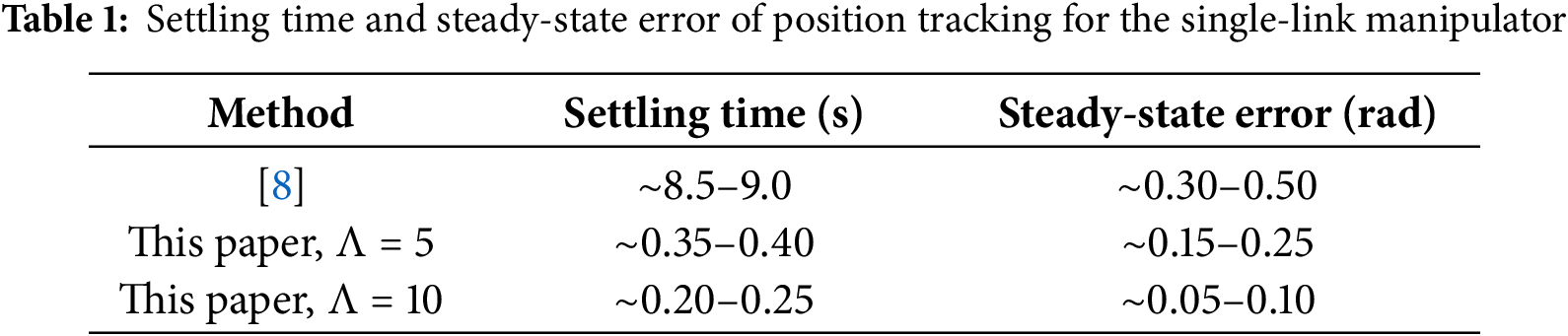
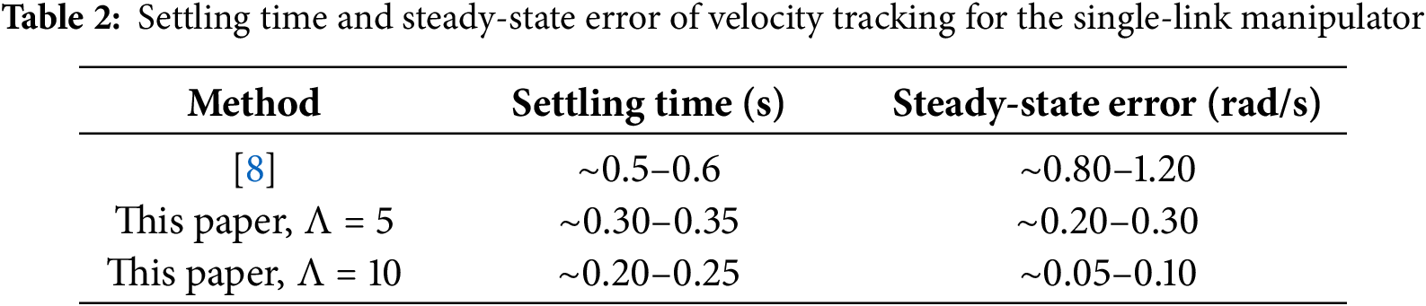
These results, summarized in Tables 1 and 2, substantiate that incorporating the reference error into the Optimal+RL design substantially improves transient speed and reduces post-tracking error; moreover,
Influence of the Reference-Error Gain
To further investigate the influence of the reference-error gain
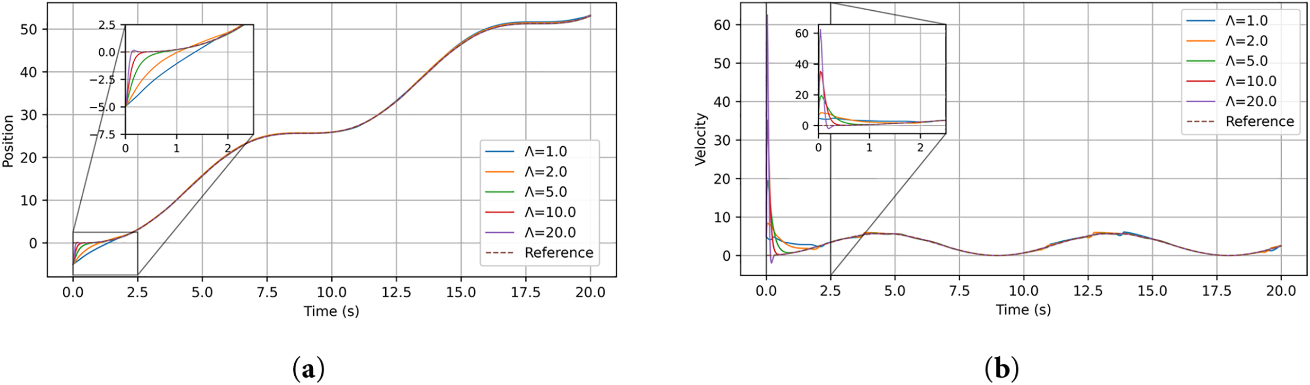
Figure 8: Position and velocity responses of the single-link manipulator under different values of the reference-error gain: (a) joint position; (b) joint velocity
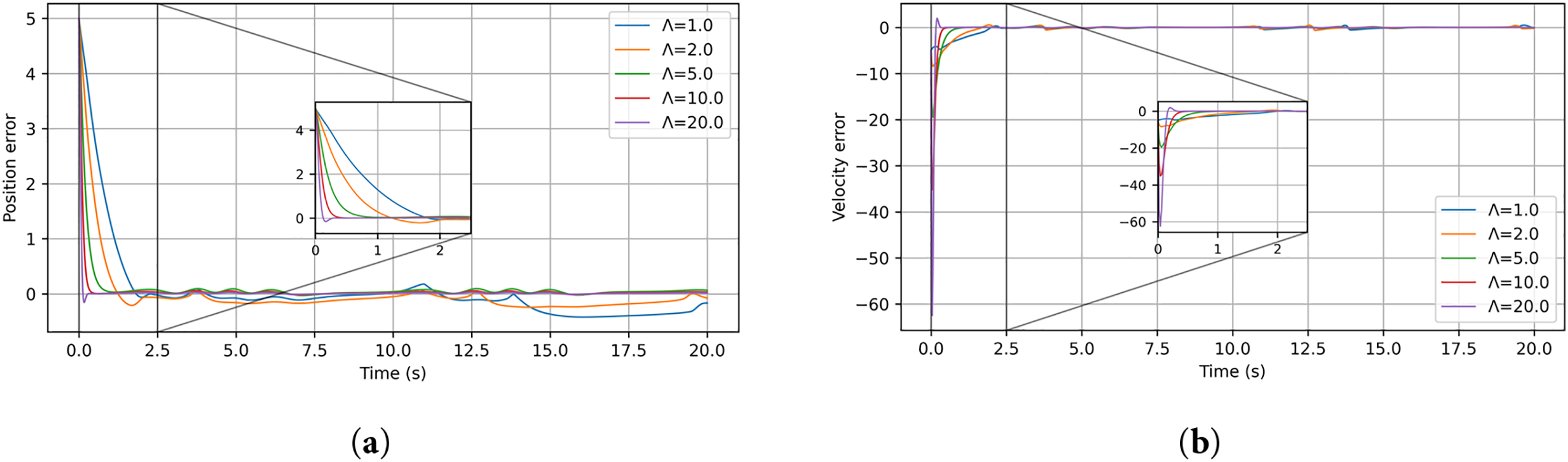
Figure 9: Position and velocity tracking errors of the single-link manipulator under different values of the reference-error gain: (a) position error; (b) velocity error
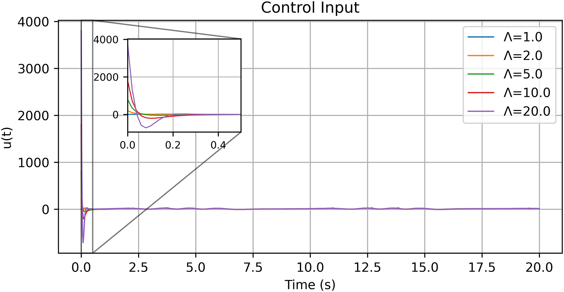
Figure 10: Control input of the single-link manipulator under different values of the reference-error gain
The cases
These observations confirm that
5.2 Nonlinear Mass–Spring–Damper
The second experiment considers a single-Degrees of Freedom (DOF) nonlinear oscillator described by
with damping
the initial condition is
For function approximation, an RBFNN with 36 Gaussian nodes is used centers on
Three tests are performed under identical settings: the method in [8], and the method proposed in this paper using Eq. (3) with
As in Section 5.1, the baseline controller from [8] in this example is also reimplemented using exactly the same controller parameters as the proposed method, so that the comparison is carried out under identical settings.
The position and velocity tracking responses of the three controllers are shown in Fig. 11, and the corresponding tracking errors are plotted in Fig. 12. The control inputs generated by the proposed method and the baseline are depicted in Fig. 13. The evolution of the actor and critic weight norms is illustrated in Figs. 14 and 15, and the associated cost function trajectories are reported in Fig. 16. The settling time and steady-state error of the position and velocity tracking are summarized in Tables 3 and 4, respectively.
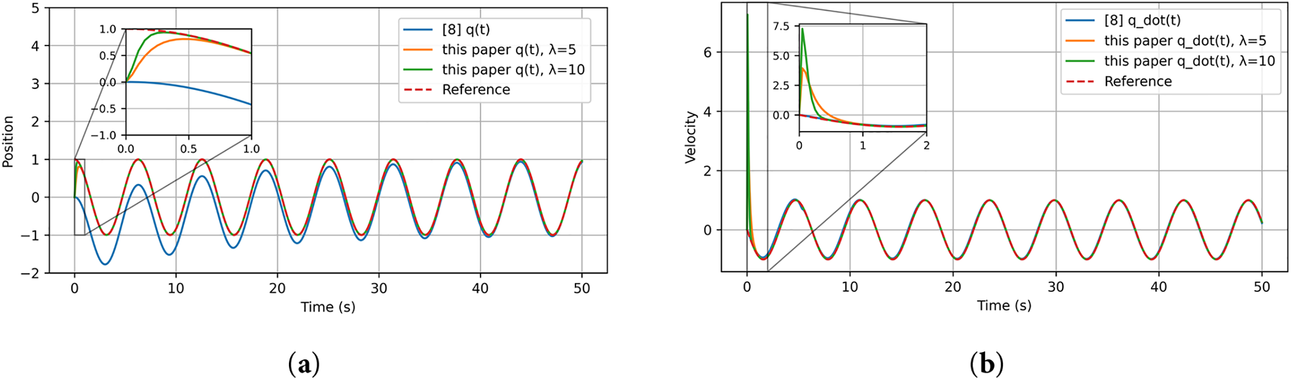
Figure 11: Position and velocity tracking of the nonlinear mass–spring–damper system: (a) position comparison between the method in [8] and the proposed method; (b) velocity comparison between the method in [8] and the proposed method. All curves are obtained from our own simulations based on the reference setup in [8]
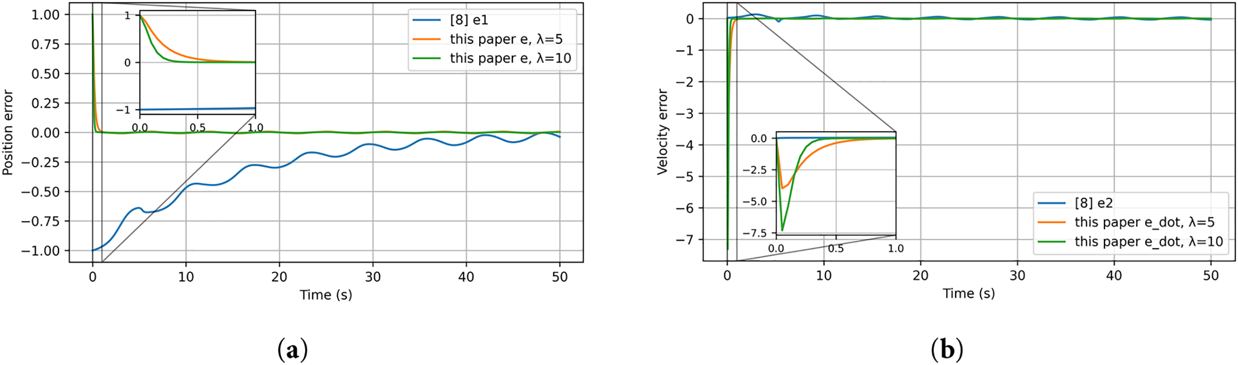
Figure 12: Tracking errors of the nonlinear mass–spring–damper system: (a) position error; (b) velocity error [8]
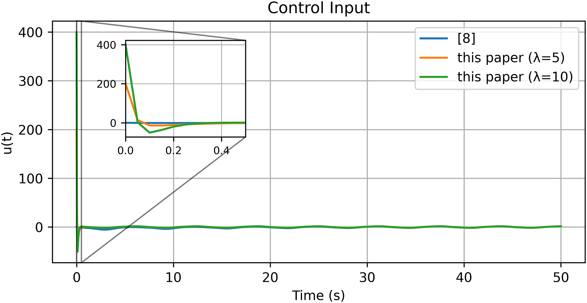
Figure 13: Control input [8]
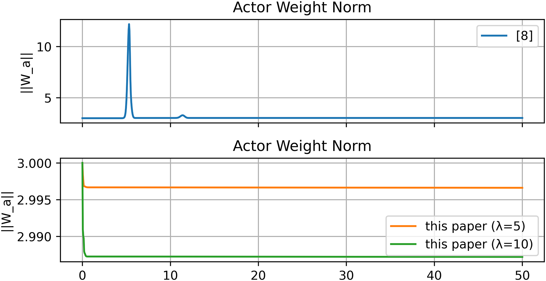
Figure 14: Norm of actor NN weights [8]
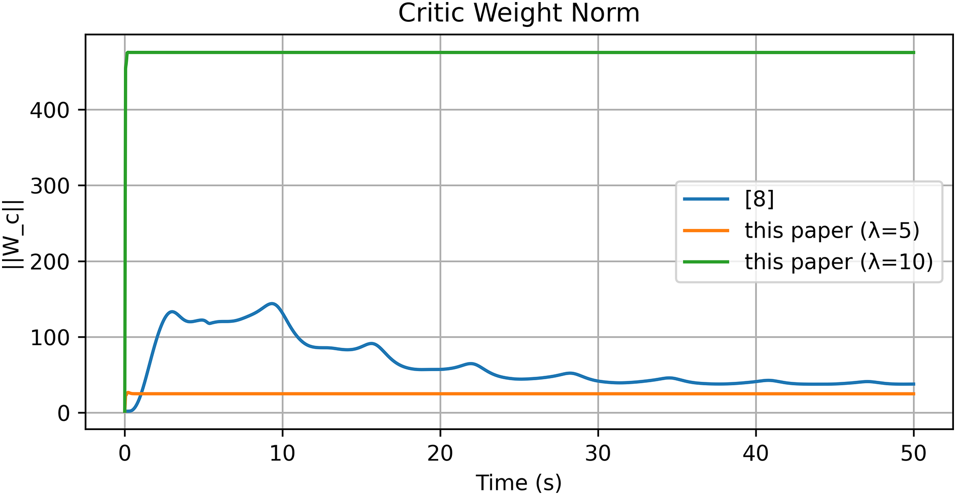
Figure 15: Norm of critic NN weights [8]
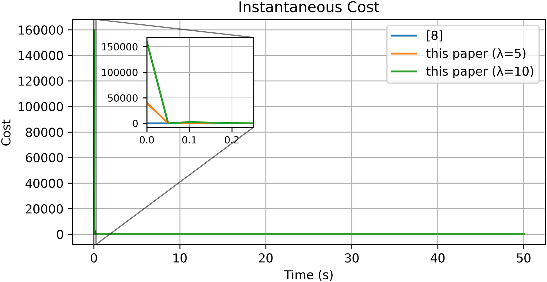
Figure 16: Cost function [8]
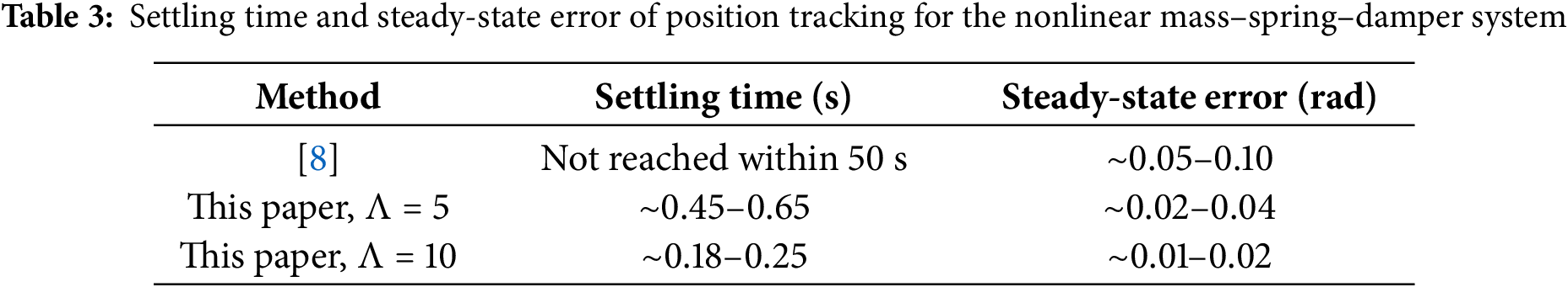
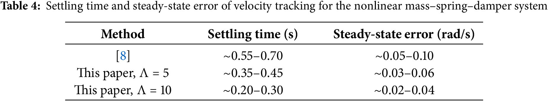
From Figs. 11–16 and Tables 3 and 4, the method in [8] shows poor performance under the chosen nonlinear reference, whereas the proposed reference-error based design achieves faster convergence, smaller steady-state errors, and smoother control effort, as visible in the insets of the velocity and torque plots.
6 Simulation in Virtual Environment—Single-Link Manipulator
To further evaluate the proposed optimal reinforcement learning control strategy, a virtual simulation platform was constructed in the Gazebo environment, which provides physics-based visualization and real-time dynamic interaction. The manipulator model and control framework were configured following the experimental setup described in [15], where the same single-link robotic system was adopted as a benchmark for validation.
The developed Gazebo environment and manipulator model are illustrated in Fig. 17, which replicates realistic joint friction, gravitational effects, and torque constraints.
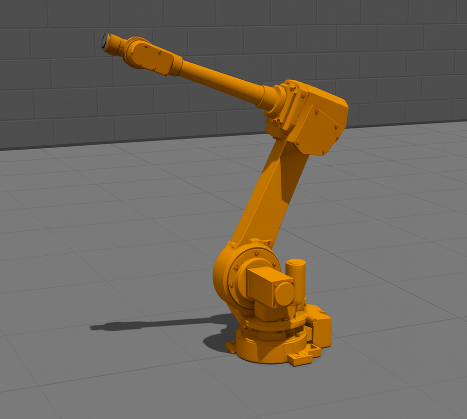
Figure 17: Gazebo simulation environment of the single-link robotic manipulator
The plant dynamics follow the model of Eq. (1):
the parameters are set as
The reference trajectory and its derivatives are defined as follows:
Simulation settings are summarized below:
The time horizon is
In this example, the baseline method of [8] is implemented with the same controller-related parameters as the proposed scheme, including the discount factor, learning rates, RBFNN structure, initial weight vectors and initial state, ensuring that both controllers are tested under the same conditions.
The results obtained in the Gazebo environment are presented in Figs. 18–23. The tracking response in Fig. 18a,b demonstrates that the proposed controller achieves accurate and stable motion tracking, closely following the desired trajectory under virtual dynamics. The position and velocity errors shown in Fig. 19a,b converge rapidly to zero, verifying that the controller maintains robustness and precision even with virtual actuator dynamics and friction. The control input shown in Fig. 20 remains smooth and bounded throughout the operation, indicating that the control effort required in the simulated environment is practical and stable. The evolution of actor and critic weights in Figs. 21–22 remains bounded, confirming the stability and learning consistency of the proposed actor–critic mechanism during the entire simulation.
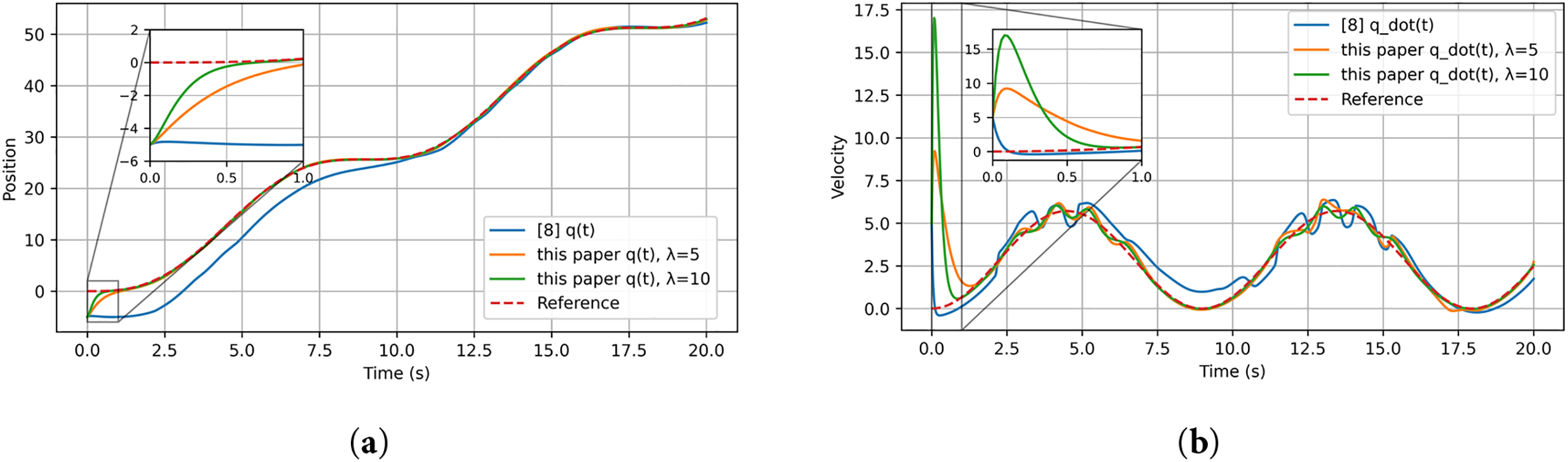
Figure 18: Position and velocity tracking of the single-link manipulator: (a) position comparison between the method in [8] and the proposed method; (b) velocity comparison between the method in [8] and the proposed method. All curves are generated from our own simulations based on the controller structure reported in [8]
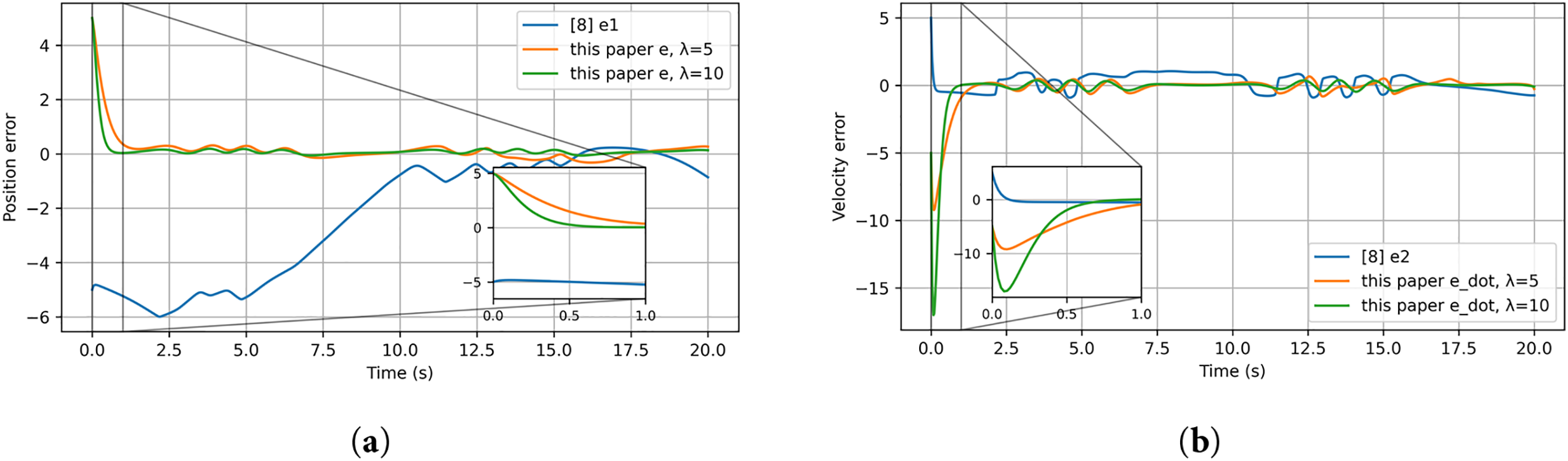
Figure 19: Tracking errors of the single-link manipulator: (a) position error; (b) velocity error [8]
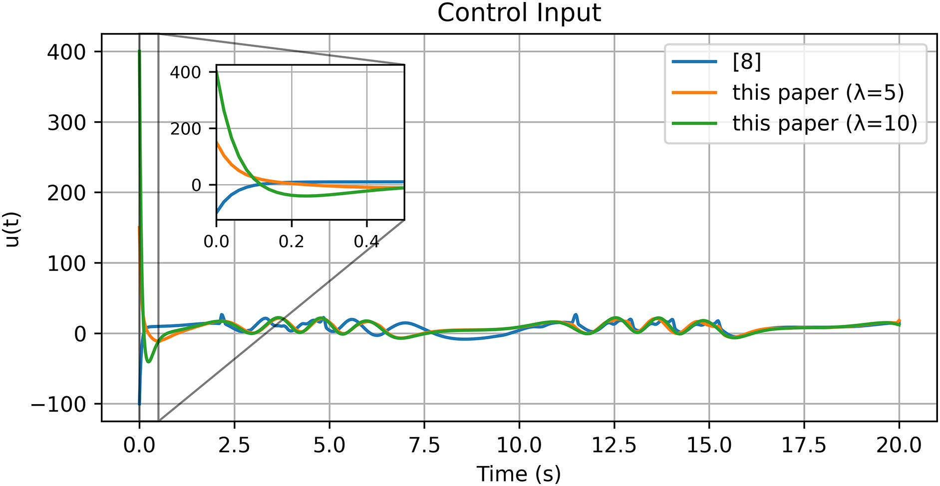
Figure 20: Control input [8]
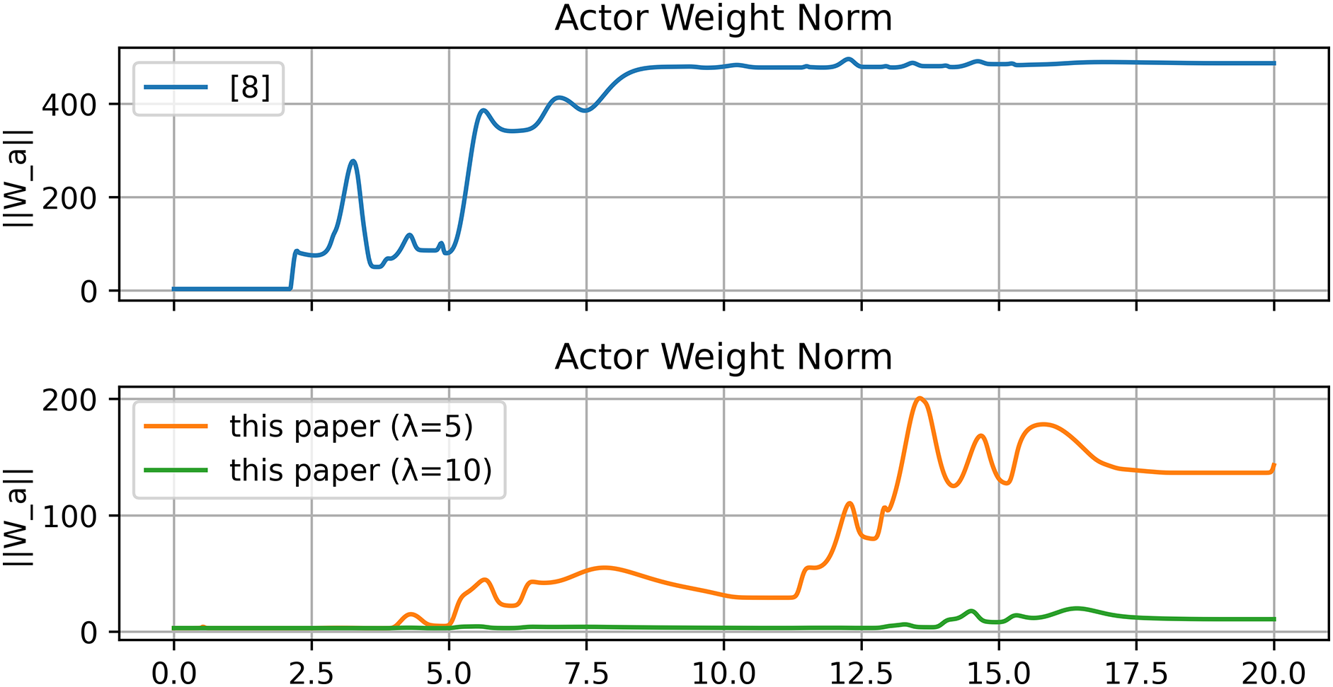
Figure 21: Norm of actor NN weights [8]

Figure 22: Norm of critic NN weights [8]
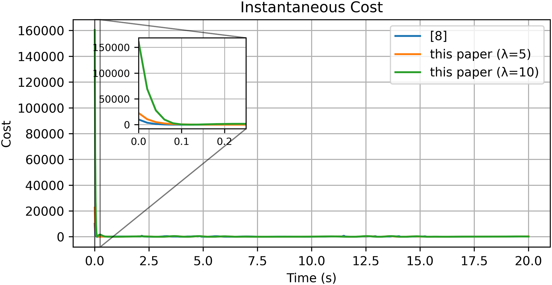
Figure 23: Cost function [8]
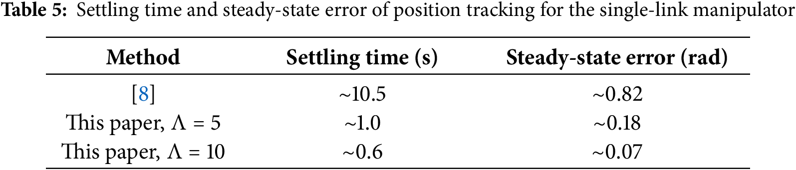
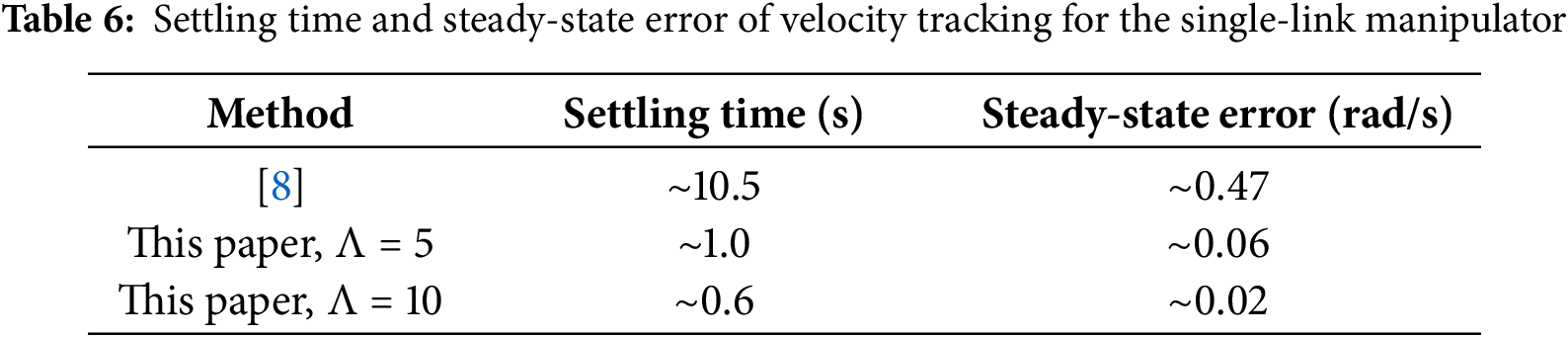
The quantitative performance evaluation is summarized in Tables 5 and 6, showing that the proposed controller significantly improves both transient and steady-state accuracy compared with the benchmark approach [8]. The results verify that the actor–critic optimal control strategy can be effectively implemented in a physics-based virtual manipulator and maintains stable adaptation during real-time operation.
In summary, the Gazebo-based virtual validation confirms the effectiveness and practicality of the proposed controller. The system maintains stable adaptation, bounded control input, and high tracking precision under realistic simulation conditions. The cost function convergence further verifies that the control policy achieves near-optimal performance while ensuring smooth and efficient actuation. These findings demonstrate that the control algorithm can be reliably extended from numerical experiments to physical robotic platforms with consistent performance.
Quantitatively, the proposed method reduces settling time by approximately 90% and steady-state error by 85% compared to [8], confirming the improved real-time performance.
This paper presented an actor–critic optimal tracking framework for nonlinear systems that augments the classical tracking error with a reference error. By reformulating the plant dynamics in the composite error state, the proposed method enables explicit shaping of the convergence rate through the gain
Simulation studies on two benchmarks—a single-link robotic manipulator and a nonlinear mass–spring–damper—demonstrated clear performance gains over the reference approach in [8]. With identical neural approximators and learning gains, the proposed controller achieved substantially faster transients and smaller steady-state errors. On the manipulator, sub-second zero-crossing of the error was obtained for
Overall, the results verify that incorporating the reference error into the Optimal+RL design offers a simple yet effective route to enhance tracking accuracy and convergence speed, without sacrificing stability guarantees. Future work will extend the method to multi-DOF manipulators and implement it on a physical UR5 robot using Robot Operating System (ROS) 2 to evaluate robustness under sensor noise and actuator saturation.
Acknowledgement: Not applicable.
Funding Statement: This work was supported in part by the National Science and Technology Council under Grant NSTC 114-2221-E-027-104.
Author Contributions: Nien-Tsu Hu: Conceptualization, Formal analysis, Funding acquisition, Methodology, Project administration, Resources, Supervision, Validation, Writing—review and editing. Hsiang-Tung Kao: Data curation, Formal analysis, Investigation, Software, Validation, Writing—original draft, Writing—review and editing. Chin-Sheng Chen and Shih-Hao Chang: Supervision, Visualization. All authors reviewed the results and approved the final version of the manuscript.
Availability of Data and Materials: The datasets and source codes generated and analyzed during the current study are not publicly available at this time but are available from the corresponding author upon reasonable request.
Ethics Approval: Not applicable.
Conflicts of Interest: The authors declare no conflicts of interest to report regarding the present study.
References
1. Ge SS, Hang CC, Zhang T. Adaptive neural network control of nonlinear systems by state and output feedback. IEEE Trans Syst, Man, Cybern B. 1999;29(6):818–28. doi:10.1109/3477.809035. [Google Scholar] [PubMed] [CrossRef]
2. Beard RW, Saridis GN, Wen JT. Galerkin approximations of the generalized Hamilton-Jacobi-Bellman equation. Automatica. 1997;33(12):2159–77. doi:10.1016/S0005-1098(97)00128-3. [Google Scholar] [CrossRef]
3. Khalil HK. Nonlinear systems. 3rd ed. Upper Saddle River, NJ, USA: Prentice Hall; 2002. 750 p. [Google Scholar]
4. Lewis FL, Vrabie DL, Syrmos VL. Optimal control. 3rd ed. Hoboken, NJ, USA: John Wiley & Sons, Inc.; 2012. 540 p. [Google Scholar]
5. Peng Z, Cheng H, Shi K, Zou C, Huang R, Li X, et al. Optimal tracking control for motion constrained robot systems via event-sampled critic learning. Expert Syst Appl. 2023;234:121085. doi:10.1016/j.eswa.2023.121085. [Google Scholar] [CrossRef]
6. Cheng G, Dong L. Optimal control for robotic manipulators with input saturation using single critic network. In: Proceedings of the 2019 Chinese Automation Congress (CAC); 2019 Nov 22–24; Hangzhou, China. p. 2344–9. doi:10.1109/cac48633.2019.8996999. [Google Scholar] [CrossRef]
7. Hu Y, Cui L, Chai S. Optimal tracking control for robotic manipulator using actor-critic network. In: Proceedings of the 2021 40th Chinese Control Conference (CCC); 2021 Jul 26–28; Shanghai, China. p. 1556–61. [Google Scholar]
8. Wen G, Philip Chen CL, Ge SS, Yang H, Liu X. Optimized adaptive nonlinear tracking control using actor–critic reinforcement learning strategy. IEEE Trans Ind Inf. 2019;15(9):4969–77. doi:10.1109/tii.2019.2894282. [Google Scholar] [CrossRef]
9. Wen G, Ge SS, Tu F. Optimized backstepping for tracking control of strict-feedback systems. IEEE Trans Neural Netw Learn Syst. 2018;29(8):3850–62. doi:10.1109/TNNLS.2018.2803726. [Google Scholar] [PubMed] [CrossRef]
10. Wen G, Philip Chen CL, Feng J, Zhou N. Optimized multi-agent formation control based on an identifier–actor–critic reinforcement learning algorithm. IEEE Trans Fuzzy Syst. 2018;26(5):2719–31. doi:10.1109/tfuzz.2017.2787561. [Google Scholar] [CrossRef]
11. Kim YH, Lewis FL, Dawson DM. Intelligent optimal control of robotic manipulators using neural networks. Automatica. 2000;36(9):1355–64. doi:10.1016/S0005-1098(00)00045-5. [Google Scholar] [CrossRef]
12. Bu X. Prescribed performance control approaches, applications and challenges: a comprehensive survey. Asian J Control. 2023;25(1):241–61. doi:10.1002/asjc.2765. [Google Scholar] [CrossRef]
13. Ghanooni P, Habibi H, Yazdani A, Wang H, MahmoudZadeh S, Ferrara A. Prescribed performance control of a robotic manipulator with unknown control gain and assigned settling time. ISA Trans. 2024;145(2):330–54. doi:10.1016/j.isatra.2023.12.011. [Google Scholar] [PubMed] [CrossRef]
14. Zhao K, Xie Y, Xu S, Zhang L. Adaptive neural appointed-time prescribed performance control for the manipulator system via barrier Lyapunov function. J Frankl Inst. 2025;362(2):107468. doi:10.1016/j.jfranklin.2024.107468. [Google Scholar] [CrossRef]
15. Rahimi F, Ziaei S, Esfanjani RM. A reinforcement learning-based control approach for tracking problem of a class of nonlinear systems: applied to a single-link manipulator. In: Proceedings of the 2023 31st International Conference on Electrical Engineering (ICEE); 2023 May 9–11; Tehran, Iran. p. 58–63. doi:10.1109/icee59167.2023.10334874. [Google Scholar] [CrossRef]
16. Rahimi Nohooji H, Zaraki A, Voos H. Actor–critic learning based PID control for robotic manipulators. Appl Soft Comput. 2024;151:111153. doi:10.1016/j.asoc.2023.111153. [Google Scholar] [CrossRef]
17. Zhao X, Han S, Tao B, Yin Z, Ding H. Model-based actor–critic learning of robotic impedance control in complex interactive environment. IEEE Trans Ind Electron. 2022;69(12):13225–35. doi:10.1109/tie.2021.3134082. [Google Scholar] [CrossRef]
18. Nam D, Huy D. H∞ tracking control for perturbed discrete-time systems using On/Off policy Q-learning algorithms. Chaos Solitons Fractals. 2025;197:116459. doi:10.1016/j.chaos.2025.116459. [Google Scholar] [CrossRef]
19. Dao PN, Nguyen VQ, Duc HAN. Nonlinear RISE based integral reinforcement learning algorithms for perturbed Bilateral Teleoperators with variable time delay. Neurocomputing. 2024;605:128355. doi:10.1016/j.neucom.2024.128355. [Google Scholar] [CrossRef]
20. Zhao JG, Chen FF. Off-policy integral reinforcement learning-based optimal tracking control for a class of nonzero-sum game systems with unknown dynamics. Optim Control Appl Meth. 2022;43(6):1623–44. doi:10.1002/oca.2916. [Google Scholar] [CrossRef]
21. Liu C, Zhao Z, Wen G. Adaptive neural network control with optimal number of hidden nodes for trajectory tracking of robot manipulators. Neurocomputing. 2019;350:136–45. doi:10.1016/j.neucom.2019.03.043. [Google Scholar] [CrossRef]
22. Vamvoudakis KG, Lewis FL. Online actor–critic algorithm to solve the continuous-time infinite horizon optimal control problem. Automatica. 2010;46(5):878–88. doi:10.1016/j.automatica.2010.02.018. [Google Scholar] [CrossRef]
Cite This Article
 Copyright © 2026 The Author(s). Published by Tech Science Press.
This work is licensed under a Creative Commons Attribution 4.0 International License , which permits unrestricted use, distribution, and reproduction in any medium, provided the original work is properly cited.
 Downloads
 Citation Tools