Fuzzy C-Means Clustering-Driven Pooling for Robust and Generalizable Convolutional Neural Networks

1  Introduction

Deep learning has brought remarkable progress in many fields by learning to extract and organize useful features from data step by step. Within this trend, convolutional neural networks (CNNs) have become the main driving force behind top performance in tasks such as image classification, object detection, and segmentation [1,2]. They are now actively applied to demanding areas like medical imaging and industrial inspection. In real-world applications, however, what matters is not only high accuracy but also predictions that can be reliable. This requires probability estimates that are well-calibrated and models that degrade gracefully when data are noisy or perturbed [3]. Such properties strongly depend on how the intermediate feature representations are formed [4–6]. In short, these trends highlight the need for architectural improvements that prevent information loss when intermediate representations are spatially subsampled [7,8].

CNN is a neural architecture introduced by LeNet-5, proposed by LeCun et al. in 1998, consisting of convolutional layers, downsampling stages, and a subsequent classification head [1] as shown in Fig. 1. Since then, subsampling has served as a key design axis for reducing the spatial dimensionality of inputs at each stage. With the introduction of ImageNet, AlexNet and VGG established max pooling between blocks as the de facto standard for rapidly shrinking per-stage inputs [2,9], while Network in Network popularized global average pooling (GAP) at the head for the final reduction [10]. GoogLeNet combined stride and pooling within multi-scale Inception paths to control per-stage input size, refined in v2/v3 with factorized convolutions and stronger normalization/optimization [11,12]. Inception-v4 and Inception-ResNet fused Inception blocks with residual connections, further strengthening learnable downsampling [13]. The All-CNN family showed that stride-2 convolutions alone can replace fixed pooling with little loss [14], and ResNet made such stride-based transitions standard via identity shortcuts [15]. Under efficiency goals, EfficientNet used depthwise stride-2 operators for spatial reduction [16] and squeeze-and-excitation (SE) and spatial attention modules for channel recalibration and feature refinement [17,18], leaving only a final GAP. More recently, ConvNeXt and ViT minimize or remove local pooling and perform dimensionality reduction via patch embeddings and hierarchical merging [19,20]. In summary, subsampling is a core axis that decides how much to reduce each layer’s input, and its mechanism has shifted from fixed rules to learnable operators.

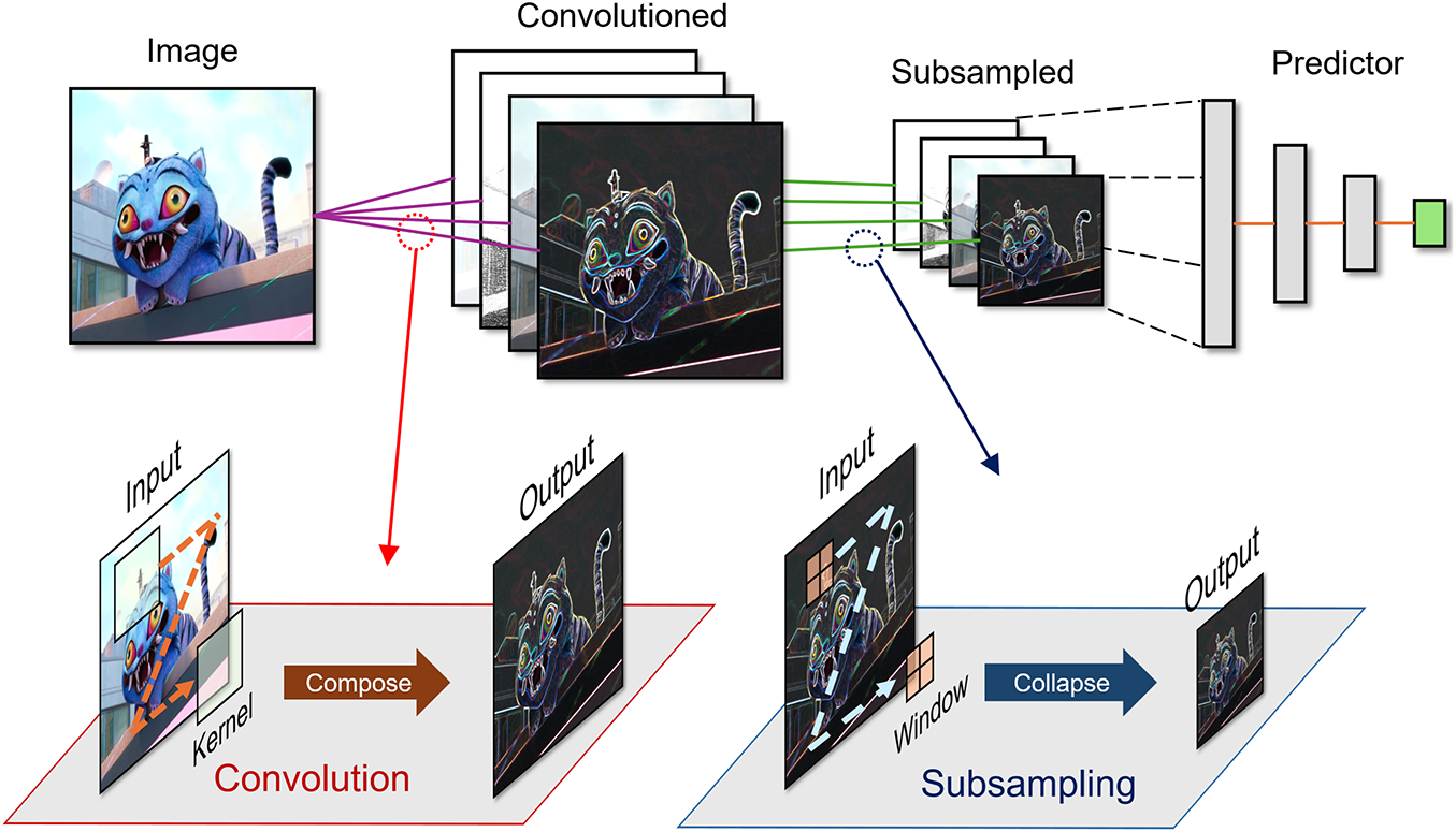
Figure 1: Overview of convolutional neural network and its major components

Among the core components of CNNs, the subsampling stage reduces the spatial size of convolutional feature maps, lowers computational cost, and helps mitigate overfitting [7]. Although many modern backbones now downsample primarily with strided convolutions, the operation that condenses local evidence remains important. Max and average pooling summarize each neighborhood into a single scalar, which can blur boundary details, suppress weak yet informative signals, and miss cues near ambiguous boundaries [8]. To address these issues, adaptive reductions have been proposed. Representative examples include Lp-norm/generalized-mean (GeM) pooling, which interpolates between average-like and max-like behaviors [21–23], and stochastic/mixed pooling, which use randomization or blending to avoid overcommitment [24,25]. These methods aim to preserve fine structure, maintain discriminative cues under distribution shift or noise, and make the reduction step more data-aware.

Nonetheless, important limitations remain. Approaches that learn the pooling exponent or mixing weights, such as Lp/GeM, are prone to overfitting to training-distribution statistics; moreover, when p drifts to extreme values, the power/root operations can induce exploding or vanishing gradients, making training numerically unstable [21,22]. More fundamentally, many methods still collapse each neighborhood to a single scalar and weight primarily by magnitude or empirical rules, thereby failing to explicitly model local ambiguity and uncertainty (e.g., overlapping boundaries or weak yet informative signals) [7].

Fuzzy logic provides a principled mathematical framework for quantifying and handling ambiguity and uncertainty [26]. In the view of fuzzy set theory, a sample is not forced into a single category; instead, it is represented by a membership vector whose components lie in [0, 1] and sum to one. Thus, information that conventional pooling would collapse to a single scalar is first decomposed into a compact, multi-aspect code that can capture overlap among feature groups. Among fuzzy clustering methods, fuzzy C-means (FCM) is a widely used soft partitioning scheme: it alternates centroid estimation with membership updates, assigns higher grades to points closer to a centroid, and uses a fuzzifier m to control assignment sharpness [27,28]. Viewed this way, fuzzy clustering complements the reduction stage in CNNs. Rather than compressing a neighborhood directly along a fixed aggregation axis, one can first obtain a low-dimensional, uncertainty-aware membership code and then summarize with type-specific strengths, allowing the summary to adapt to local mixtures while remaining drop-in compatible with standard backbones. In the design studied here, each location acquires memberships to a small set of latent clusters, and the layer aggregates with cluster-specific pooling exponents.

This paper proposes a fuzzy pooling layer that estimates per-window soft memberships with FCM and aggregates activations using cluster-specific Lp exponents pk. Memberships weight the contributions of each cluster while the per-centroid exponents modulate pooling sharpness, enabling the layer to explicitly capture local ambiguity and uncertainty near boundaries. The module is drop-in compatible with standard CNNs and maintains strong performance under limited training data and unclear inter-class boundaries.

Contributions.

1.    Uncertainty-aware pooling. Introduces a FCM–driven pooling that encodes per-window soft memberships and aggregates with cluster-specific exponents, explicitly modeling local ambiguity that magnitude-based Lp/GeM or stochastic/mixed pooling do not capture.

2.    Drop-in gains across data scarcity. Demonstrates consistent improvements in accuracy and weighted F1 over conventional pooling across backbones and datasets, with the largest margins under limited supervision and subtle class boundaries.

Paper organization. Section 2 reviews pooling methods and related work and discusses their limitations. Section 3 details the design and operation of the proposed fuzzy clustering–based pooling layer. Section 4 evaluates performance across diverse setups, and Section 5 concludes with future directions.

2  Background and Related Work

Pooling in CNNs plays a structural role in shaping the feature hierarchy. By summarizing responses within a local window, it reduces spatial resolution, lowers memory footprint and computational burden, and progressively enlarges the effective receptive field. The resulting compact intermediate representations make subsequent layers more tractable and enable stable scaling from early, high-resolution maps to deeper stages [7,29]. In modern architectures, this reduction is realized either by explicit max/average pooling or by strided convolutions; in both cases, the intent is to transform dense neighborhood activations into concise, higher-level features that support efficient learning and inference [14].

2.1 Value-Based Pooling: From Static to Learned Sharpness

Static operators (max/average). For a window ℛ with activations {xi}i∈ℛ,

yavg=1|ℛ|∑i∈ℛxi,ymax=maxi∈ℛxi.(1)

As shown in Fig. 2a, max pooling selects the largest activation in each window, accentuating strong responses and providing limited shift invariance as in Eq. (1), often leading to aliasing artifacts [30]. During backpropagation, the gradient is routed only to the argmax entry, yielding sparse updates but increasing sensitivity to outliers. In contrast, as shown in Fig. 2b, average pooling spreads gradients uniformly across entries and stabilizes optimization, though it can oversmooth edges and lose boundary-level evidence [7,29].

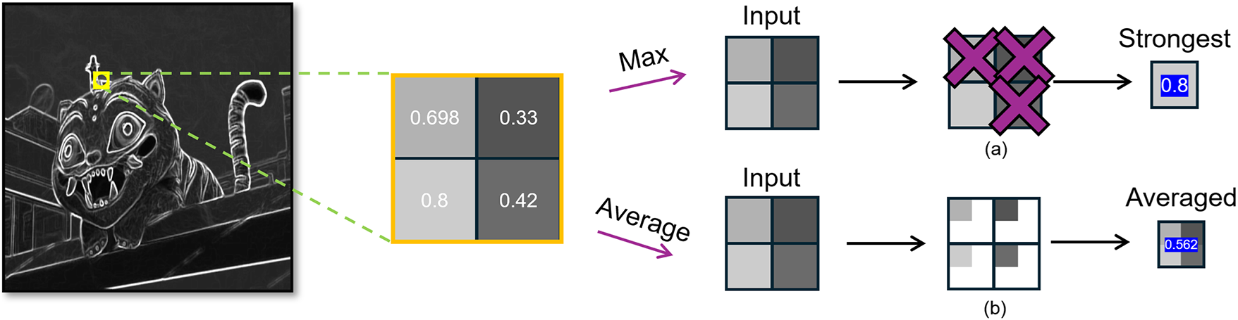
Figure 2: Traditional static pooling. (a) Max pooling keeps only the strongest response; (b) Average pooling takes the mean. Both collapse a local patch to a single scalar

Generalized-mean (Lp) pooling. The generalized mean

yLp = (1|ℛ|∑i∈ℛ|xi|p)1/p,p>0,(2)

controls pooling sharpness with a single parameter p [21–23]. In Eq. (2) when p=1, it equals average pooling; for p→∞, it approximates max pooling; and for 0<p<1, it damps outliers like a geometric mean. As illustrated in Fig. 3a, the normalized L2 case averages squared responses and then takes the square root.

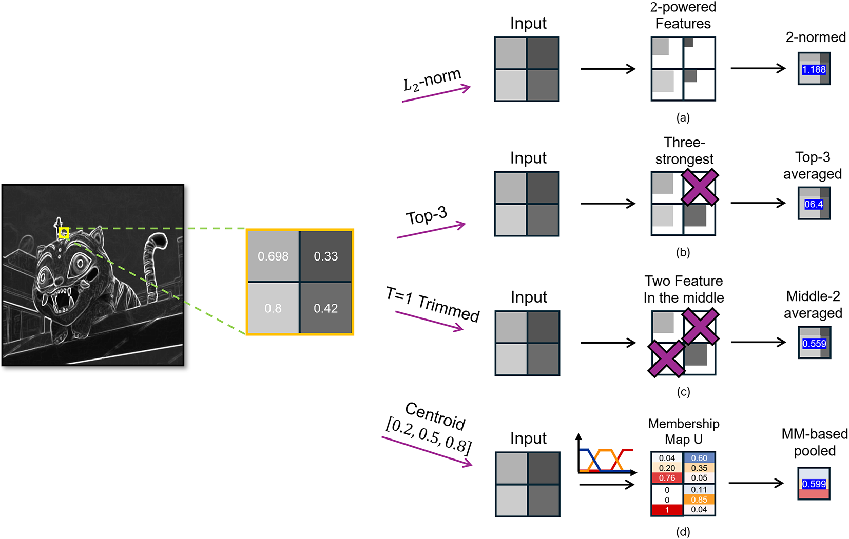
Figure 3: Soft pooling variants on a shared 2×2 neighborhood (yellow box). Each row squares the inputs and aggregates via: (a) normalized L2; (b) Top-K averaging; (c) trimmed mean; (d) Type-1 fuzzy pooling with membership functions

In practice, power-mean pooling benefits from proper normalization for both accuracy and numerical stability. Prior work on Lp/GeM reports improved performance when the pooled output is normalized (e.g., power/mean normalization or downstream normalization layers) [23]. More broadly, Batch Normalization (BN) is known to stabilize training by smoothing the loss landscape and conditioning gradients [31,32].

Order-statistic pooling. This family summarizes responses by rank rather than magnitude. As illustrated in Fig. 3b, Top-K pooling averages the K largest activations (e.g., Top-3 average pooling on a 2×2 neighborhood selects the three largest values and averages them). In Fig. 3c, a trimmed mean discards the T largest and T smallest values (e.g., T=1 on a 2×2 window, i.e., T-1 trimmed pooling), then averages the remainder. Quantile pooling instead selects a specific order statistic, such as the median. With small windows, these rank-based selection masks can change discretely when ranks swap, yielding piecewise-smooth behavior [7].

T-max-avg pooling. This hybrid keeps the maximum if the Top-K responses exceed a threshold T; otherwise, it falls back to the average of Top-K [33]. It balances noise-robustness and peak preservation, though with small windows, it often degenerates to simpler forms.

2.2 Membership-Based Pooling

Unlike value-only reductions, membership-based pooling explicitly represents local ambiguity by assigning each activation a degree of belonging in [0, 1], [26].

Type-1 (membership/rule–driven). Given activations and fixed/learned memberships, pooling is performed as a weighted average. As illustrated in Fig. 3d, learned membership functions (with centers at approximately 0.2, 0.5, and 0.8 in this example) assign weights to entries according to their degrees of belonging before aggregation. This operator is simple and differentiable, but often depends on hand-crafted or task-tuned membership functions, which can limit generality [34,35].

Fuzzy logic has also been integrated into CNN pooling mechanisms and clustering frameworks to enhance feature preservation [36]. FP-CNN [37] introduced a fuzzy pooling operator that adaptively combines max and average pooling through a membership function derived from local feature intensities. Specifically, each pooling region computes a fuzzy membership μ and aggregates responses as μ⋅max+(1−μ)⋅avg, thus balancing sharpness and smoothness while mitigating spatial information loss. Unlike this hybrid formulation, our proposed method generalizes the pooling process through a trainable, membership-driven Lp aggregation that adjusts its exponent per location, offering a more flexible and differentiable fuzzy adaptation mechanism.

Type-2 (uncertain memberships). Here, memberships themselves are uncertain, modeled as intervals with type-reduction prior to defuzzification [38]. It can improve robustness under distribution shifts, but adds complexity and hyperparameters.

Position of this work. Type-1 and Type-2 show the importance of uncertainty-aware pooling, but each faces practical challenges. Our approach addresses these by estimating memberships with FCM and aggregating with cluster-specific exponents, combining adaptability with drop-in compatibility.

3  Fuzzy Clustering–Based Soft Pooling Layer

Design rationale. The analysis in Section 2 suggests three desiderata for a modern pooling operator: (i) avoid collapsing each neighborhood to a single scalar purely by magnitude, so that ambiguous boundary evidence is not discarded; (ii) adapt the sharpness of aggregation to local patterns without the discrete switches of rank-based rules; and (iii) remain numerically stable and efficient, without incurring the overhead of heavy attention mechanisms [17,18] or spectral transforms.

3.1 Overview of the Proposed Layer

Fig. 4 summarizes the workflow of the proposed fuzzy clustering-driven soft pooling layer. Given an input feature map, we compute fuzzy memberships per sample and per location via FCM, using cluster centers shared across the batch. We then realize two pooling variants: (a) Membership Averaging and (b) Membership Maxing. Both variants ultimately perform a normalized generalized-mean (Lp) aggregation whose exponent is adapted per spatial location.

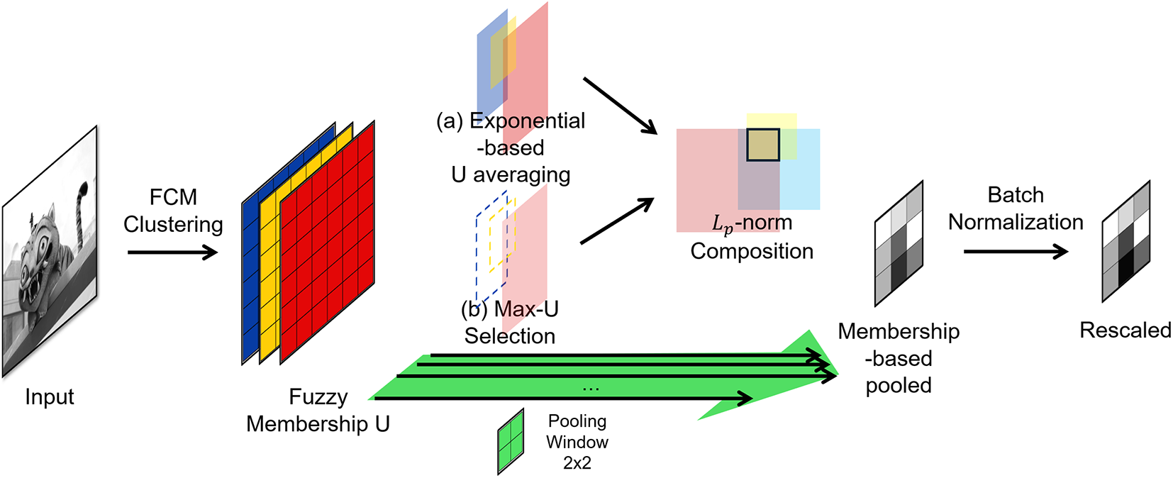
Figure 4: Overview of the proposed fuzzy clustering–based soft pooling layer. FCM yields a per-location membership map U over K latent types. Two branches set the pooling exponent: (a) Membership Averaging and (b) Membership Maxing. The resulting pij guides a normalized Lpij aggregation, followed by BN-style normalization

In practice, the proposed fuzzy pooling layer directly follows each convolutional block, taking its feature map as input without any intermediate transformation. The output retains the same channel dimension and is passed to the next convolution or fully connected layer. Thus, it functions as a drop-in replacement for conventional Max or Average pooling within standard CNN architectures.

3.2 Input Structure and Clustering

Assume a feature tensor X∈RB×H×W×C and let xb,ij∈RC denote the C-dimensional feature at spatial location (i,j) in sample b. And also let {ck}k=1K denote trainable cluster centers in RC (shared across the batch). Define the per-sample, per-location, per-cluster distance as in Eq. (3).

db,ij,k = ‖xb,ij−ck‖2+ε,(3)

where ε>0 avoids division by zero. With fuzzifier m>1, the memberships are defined following the standard FCM formulation [28] as in Eq. (4).

ub,ij,k = (∑ℓ=1K(db,ij,kdb,ij,ℓ)2m−1)−1,s.t.∑k=1Kub,ij,k=1,(4)

yielding a membership tensor U∈[0,1]B×H×W×K. The centers {ck} are optimized end-to-end via backpropagation.

3.3 Computation of the Pooling Exponent

Each cluster k is associated with a learnable exponent pk. We constrain pk∈[pmin,pmax] via a squashed parameterization as in Eq. (5).

pk = pmin+σ(p~k)(pmax−pmin),(5)

where p~k is the unbounded learnable parameter and σ(⋅) is the sigmoid function.

Given the memberships {ub,ij,k} and cluster exponents {pk}, the per-location exponent pb,ij is determined by one of the following two schemes as in Eqs. (6) and (7).

(a) Membership Averaging:pb,ij = ∑k=1Kub,ij,kpk,(6)

(b) Membership Maxing:pb,ij = pk⋆,where k⋆ = arg maxkub,ij,k.(7)

Interpretation of cluster exponents. Implicitly, clusters act as latent pattern types (e.g., edges, textures, flat regions). Learning a distinct pk per type lets the layer tune aggregation sharpness to the local pattern (e.g., larger pk near salient edges, smaller pk in smooth areas) with low overhead.

Commonality vs. difference. Both rules rely on the same memberships U and type-wise exponents {pk}. Averaging is smooth and differentiable, while Maxing is simpler but introduces a discrete arg⁡max; in practice we use Averaging as default and report Maxing as an ablation.

3.4 Integration and Output

Pooling is applied per channel. Let Ωij denote the pooling window centered at (i,j) with cardinality |Ωij|. Using the computed exponent pb,ij, the output is defined as in Eq. (8).

yb,ijc = (1|Ωij|∑(m,n)∈Ωij|Xb,mnc|pb,ij)1/pb,ij,(8)

where Xb,mnc denotes the input scalar activation at location (m,n) and channel c.

Optionally, a membership-weighted variant replaces the uniform average (1/|Ωij|) with normalized weights wmn(b,ij)≥0 satisfying ∑(m,n)∈Ωijwmn(b,ij)=1.

3.5 BN-Inspired Stabilization after the Proposed Fuzzy Pooling

After the proposed fuzzy pooling, a BN-style normalization is appended to stabilize both feature scales and gradient dynamics. In fuzzy clustering-based pooling, the membership distributions {ub,ij,k} evolve spatially and temporally during training, and their interaction with the adaptive exponents pb,ij can amplify response variance within each mini-batch. This phenomenon is analogous to the local-rule dominance observed in fuzzy systems under non-uniform data distributions [34,35].

Applying BN immediately after pooling normalizes channel-wise statistics, effectively damping variance propagation and smoothing gradient flow across iterations. From a theoretical perspective, the adaptive Lp operator embedded in the proposed fuzzy pooling acts as a non-linear scaling mechanism whose sensitivity to input magnitude increases with p. BN counteracts this by rescaling activations toward unit variance, thereby maintaining consistent learning dynamics regardless of the spatially varying sharpness pb,ij. This interpretation aligns with prior findings that BN smooths the optimization landscape and stabilizes gradient propagation in deep networks [31,32].

Empirical evidence of this stabilizing effect is presented in Appendix A. Across all architectures (LeNet-5, AlexNet, and VGG-16), the BN-applied variants consistently achieved 3%–8% higher accuracy and weighted F1 scores with reduced variance, demonstrating that BN functions as a structural stabilizer within the proposed fuzzy-adaptive pooling rather than merely as a statistical normalization step. All experiments were conducted with a batch size of 32, providing sufficient samples for reliable batch statistics while avoiding the instability often observed in small-batch BN.

3.6 Illustrative Example

To clarify the computation process of the proposed fuzzy pooling layer, Fig. 5 visualizes the step-by-step operation from clustering to adaptive pooling. An input feature map is clustered by FCM into K=3 latent types, yielding a membership map U. Two paths are illustrated: (a) Membership Averaging, where the cluster-specific exponents p=[1,1.5,2] are averaged with memberships to form pij, then used for normalized Lpij pooling; (b) Membership Maxing, where the argmax membership selects a cluster per location, followed by pooling with the corresponding pij. In both cases, BN-style normalization is applied after pooling. For reference, conventional average and max pooling outputs are also shown.

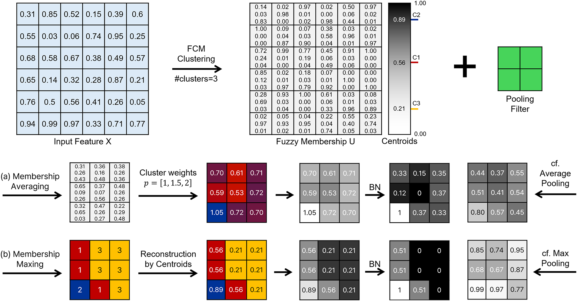
Figure 5: Step-by-step computation of the proposed fuzzy pooling layer. Top: input feature map, FCM memberships, and learned centroids. Bottom: (a) Membership Averaging and (b) Membership Maxing, each followed by BN-style normalization. For comparison, the outputs of conventional average and max pooling are also shown

To further highlight the difference from conventional pooling, Fig. 6 presents the visualized results after the 1st and 2nd pooling stages using various pooling methods. While Average and L2-norm pooling tend to smooth out detailed edges, and Max pooling overemphasizes only the highest activations, the proposed fuzzy pooling variants (Mavg and Mmax) adaptively regulate contrast based on the learned exponents p=[5,0.2,0.2]. Assuming the feature activations are normalized in [0,1], regions associated with clusters having pk>1 are suppressed (weakened), whereas those with pk<1 are enhanced (highlighted). Consequently, the darkest and brightest clusters become more prominent, while intermediate tones are attenuated, leading to stronger edge delineation and higher local contrast.

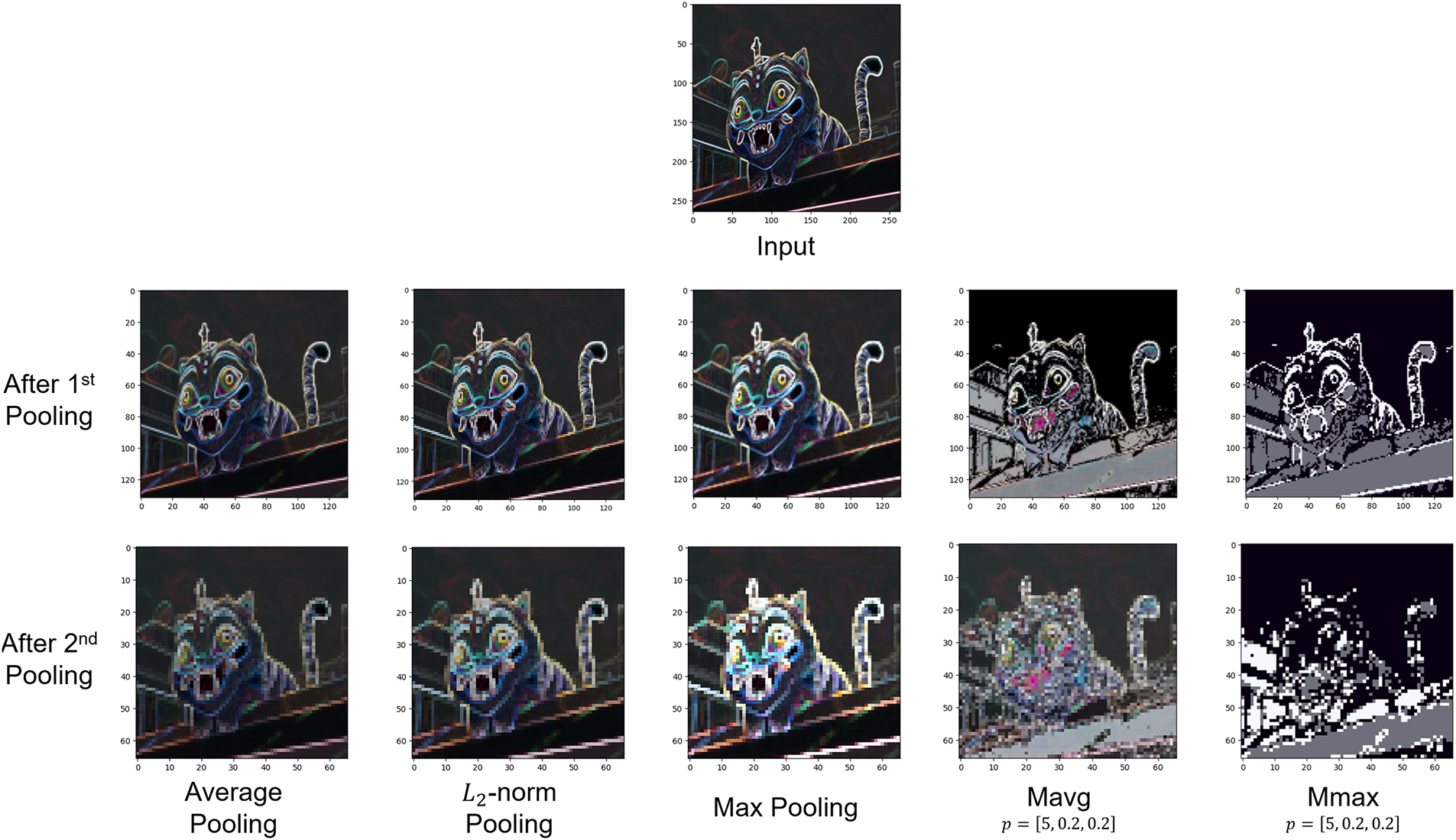
Figure 6: Visual comparison of feature maps after the first and second pooling stages across different pooling methods. Average and L2-norm pooling blur local textures, while Max pooling saturates high responses. In contrast, the proposed fuzzy pooling (Mavg, Mmax) adaptively balances enhancement and suppression through learned pk, resulting in more distinct edges and sharper feature contrast

This two-step illustration—computation flow followed by visual comparison—clarifies how the proposed fuzzy pooling mechanism translates its adaptive exponent control into perceivable structural differences. The enhanced local contrast observed here provides a visual rationale for the superior discriminative performance demonstrated in Section 4.3 and supports the need for BN stabilization discussed in Section 3.5. For further visualizations concerning the effect of the cluster count K and different integration strategies, please refer to Appendix B.

3.7 Computational Complexity Analysis

The proposed fuzzy pooling layer integrates three computational components: (1) membership estimation based on feature-to-center distances defined in Eq. (3), (2) adaptive Lp-norm aggregation guided by the learned exponents, and (3) BN-style normalization for stabilization. Each part contributes differently to the overall computational cost, which we analyze below.

Note that a classical FCM algorithm requires iterative updates with a typical complexity of 𝒪(NK2CI) or 𝒪(NKCI) for improved variants [39], where I is the number of iterations. By contrast, the proposed pooling layer performs a single-pass computation without iteration.

Membership computation. Using the distance formulation in Eq. (3), each spatial location computes its distances to K cluster centers and normalizes them according to the membership rule in Eq. (4). This operation requires 𝒪(CK) computations per location, and thus 𝒪(NCK) for the entire feature map, where N=H×W. Since cluster centers are optimized by backpropagation rather than iterative FCM updates, no additional loop over iterations is needed, keeping the process single-pass.

Adaptive pooling and normalization. Once the memberships are obtained, the per-location exponent pb,ij is computed through either the weighted averaging rule in Eq. (6) or the hard selection rule in Eq. (7). Both require at most 𝒪(NK) operations. Subsequent adaptive Lp pooling in Eq. (8) and BN-style normalization are performed channel-wise, each with 𝒪(NC) complexity.

Overall complexity. Summing these components, the overall computational cost of the proposed layer is 𝒪(NCK), dominated by the membership computation step. For comparison, standard average or max pooling has 𝒪(NC) complexity. Therefore, the proposed fuzzy pooling introduces only a small linear factor of K to model fuzzy memberships and adaptive aggregation strength, while maintaining computational feasibility for modern CNN architectures.

Empirical inference efficiency. To complement the asymptotic analysis, we measured the actual inference time per batch (32 samples) across representative CNNs and pooling methods. Table 1 summarizes the results averaged over five runs.

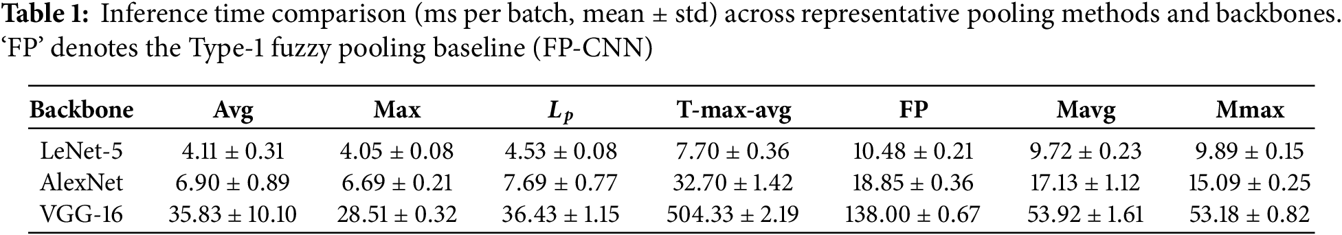
The inference latency of the proposed fuzzy pooling (Mavg and Mmax) is generally comparable to that of the Type-1 fuzzy baseline (FP) on smaller networks, while being substantially faster on the deeper VGG-16 architecture (e.g., ∼2.5× speedup over FP). Both variants are also significantly more efficient than the sorting-intensive T-max-avg operator. Although slightly slower than classical average or max pooling due to membership estimation, the proposed methods maintain a favorable trade-off between representational robustness and computational efficiency. Importantly, the gap between Mavg and Mmax remains within statistical variance, suggesting that their inference complexity is nearly identical despite their different exponent selection rules. This confirms the proposed design’s suitability for real-time or on-device deployment across CNN architectures of various depths.

4  Implementation and Evaluation

4.1 Experimental Environment and Setup

We evaluate the pooling layers defined in Section 3 in two distinct experimental phases against seven alternatives.

Hardware configuration.

All experiments were conducted on a workstation equipped with an Intel Core i9-13900F CPU (24 cores, 32 threads), an NVIDIA RTX 4090 GPU (24 GB VRAM), and 64 GB of main memory. TensorFlow (ver. 2.12) was used with the NVIDIA-recommended configuration for the RTX 4090, including CUDA 12.x and cuDNN 8.x libraries. The batch size was fixed at 32 across all experiments to ensure consistent batch-normalization statistics and reproducible inference-time comparisons.

Proposed methods. Mavg: Membership-Averaging fuzzy pooling; Mmax: Membership-Maxing fuzzy pooling. Both variants incorporate the BN-style stabilization described in Section 3 (ablation study provided in Appendix A).

Baselines. To validate effectiveness, we compare against seven pooling strategies: Max and Avg pooling (standard); Lp: generalized-mean pooling with learnable p [21]; T-max-avg: thresholded Top-K hybrid discussed in Section 2.1 [33]; Type-1 fixed: Type-1 fuzzy pooling with a fixed membership function (e.g., triangular/Gaussian) [34]; Type-1 learnable: Type-1 fuzzy pooling with trainable membership parameters; and FP: the fuzzy-pooling module from FP-CNN [37], representing a prior convolution-integrated fuzzy pooling framework.

Backbones and insertion points.

We use three CNN backbones, as illustrated in Fig. 7: (a) LeNet-5 [1], (b) AlexNet [2], and (c) VGG-16 [9]. In all models, the native pooling layers (highlighted in green) are replaced one-for-one by each candidate pooling operator, preserving the original window size, stride, and padding configuration.

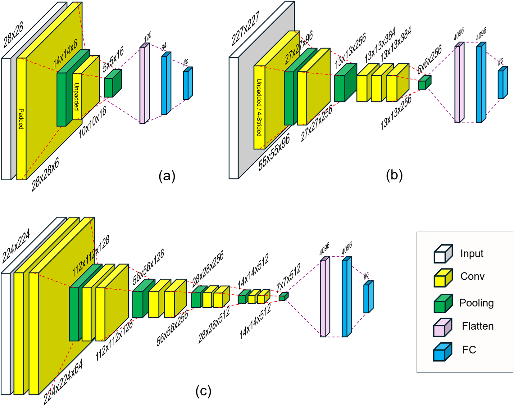
Figure 7: Backbone CNNs and pooling insertion points. (a) LeNet-5-style network for 28×28 inputs (two conv blocks → two pooling stages → FC). (b) AlexNet-style network for 224×224 inputs. (c) VGG-16-style network with five pooling stages. Green blocks indicate where native pooling is swapped with one of {Max, Avg, Lp, T-max-avg, Type-1 fixed, Type-1 learnable, Mavg, Mmax}

Why hold-out (HO) instead of k-fold CV.

While k-fold cross-validation is standard practice, we observed that several traditional pooling baselines occasionally exhibited numerical instability or convergence failure (e.g., loss divergence or stagnation) under identical training protocols. Since such instability renders the corresponding folds statistically unreliable and practically undeployable, including them introduces unnecessary volatility into the comparison. Therefore, we adopt a repeated hold-out evaluation protocol and aggregate results only from successfully converged runs to ensure a fair assessment of peak capability (convergence criteria detailed below).

Experiment 1 (Multi-backbone comparison).

This phase evaluates general classification performance across diverse domains.

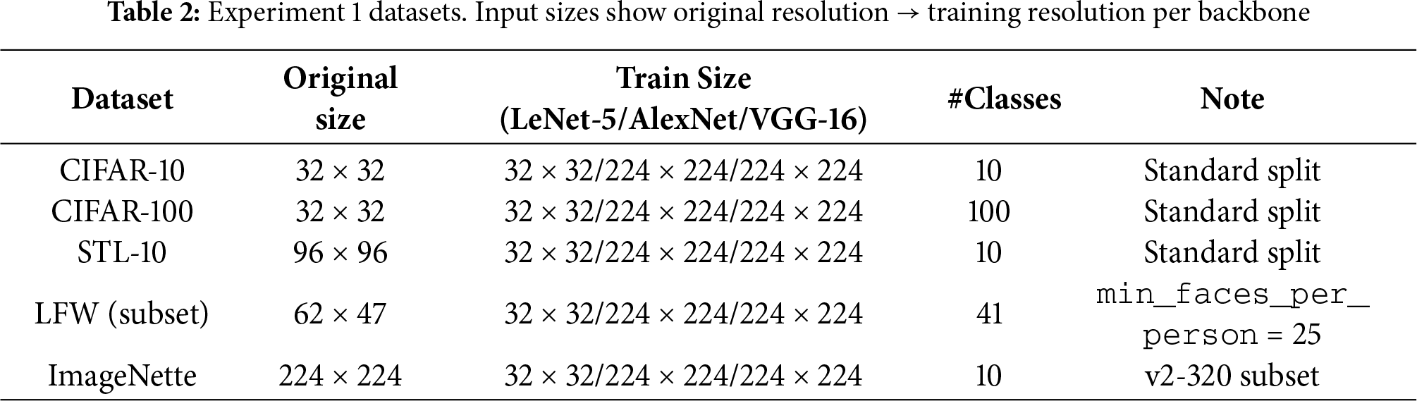
•   Datasets: CIFAR-10 and CIFAR-100 [40], LFW (subset) [41], STL-10 [42], and ImageNette (a subset of ImageNet [43]), as summarized in Table 2.

•   Split: A single random hold-out (HO) partition with a ratio of train:val:test = 0.6:0.2:0.2.

•   Backbones: LeNet-5, AlexNet, and VGG-16.

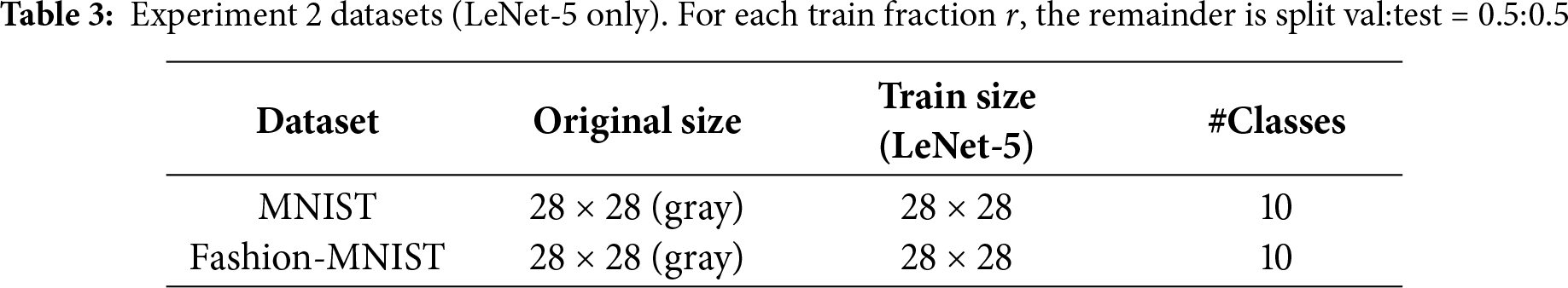
Experiment 2 (Low-resolution, low-data probe).

This phase probes robustness under data scarcity using lightweight models.

•   Backbone: LeNet-5 only (input resized to 28×28).

•   Datasets: MNIST [1] and Fashion-MNIST [44], as summarized in Table 3.

•   Split: For each training fraction r∈{0.001,0.002,0.005,0.01,0.02,0.05,0.1,0.2,0.5}, we sample the training set at proportion r and split the remainder equally into val:test = 0.5:0.5.

Repeated HO with convergence filtering.

For each (dataset, backbone, pooling) configuration, we draw independent random HO partitions and train until obtaining a fixed number of converged runs: 10 runs for Experiment 1 and 5 runs for Experiment 2. Runs that do not converge (e.g., due to divergence or instability) are discarded and retried with a new random seed and split. We report the mean ± standard deviation calculated over these retained, successful runs.

Preprocessing and training.

Inputs are min-max normalized to [0,1], and targets use one-hot encoding with a label smoothing factor of 0.25. Training employs the Adam optimizer with a learning rate of 4×10−4 (decaying by 0.1 on plateaus) for 100 epochs, utilizing categorical cross-entropy loss. Experiment 1 resolutions vary by backbone: LeNet-5 uses 32×32 RGB (first conv adapted to 3 channels), while AlexNet and VGG-16 use 224×224. Experiment 2 uses native 28×28 grayscale for LeNet-5. Unless otherwise noted, the number of clusters K in Mavg/Mmax is set equal to the number of classes for the dataset.

Hyperparameter setting for m and K.

The fuzzifier was fixed at m=2.0 in all experiments, following common practice in FCM-based models [28], which provides stable and moderately soft memberships for visual feature maps.

To determine a suitable range for the number of clusters K, we conducted preliminary experiments under conditions similar to the two main setups (Training ratio Tr=0.6 in Experiment 1 and Tr=0.001 in Experiment 2) on representative datasets. Varying K from 2 to 9 revealed that the proposed method is generally robust to K, showing no statistically significant performance degradation across this range.

In the main experiments, to ensure optimal model selection, K was determined based on the validation loss during the stabilization phase of training—the intermediate stage where training and validation losses oscillate around equilibrium before overfitting begins. This phase, which follows the initial rapid convergence and precedes the divergence between training and validation losses, best reflects the model’s saturated generalization capability. Accordingly, we monitored the validation loss over the last 10 epochs of this phase and selected the K yielding the lowest validation loss. This procedure provides a data-driven and reproducible determination of K, avoiding bias from transient states.

4.2 Results

Experiment 1 (Multi-backbone).

Figs. 8–13 present the accuracy and weighted F1 distributions (10 converged hold-out runs) for LeNet-5, AlexNet, and VGG-16. Across all configurations, Mavg and Mmax consistently achieve the highest medians (or tie for the top position) with narrower interquartile ranges (IQRs), indicating robust convergence. Notably, these improvements are statistically significant (Wilcoxon signed-rank test, p<0.05) against the strongest baselines in most cases. In contrast, the Type-1 fuzzy and FP-CNN baselines generally yield lower medians and larger variability, highlighting the advantage of the proposed cluster-specific exponent adaptation.

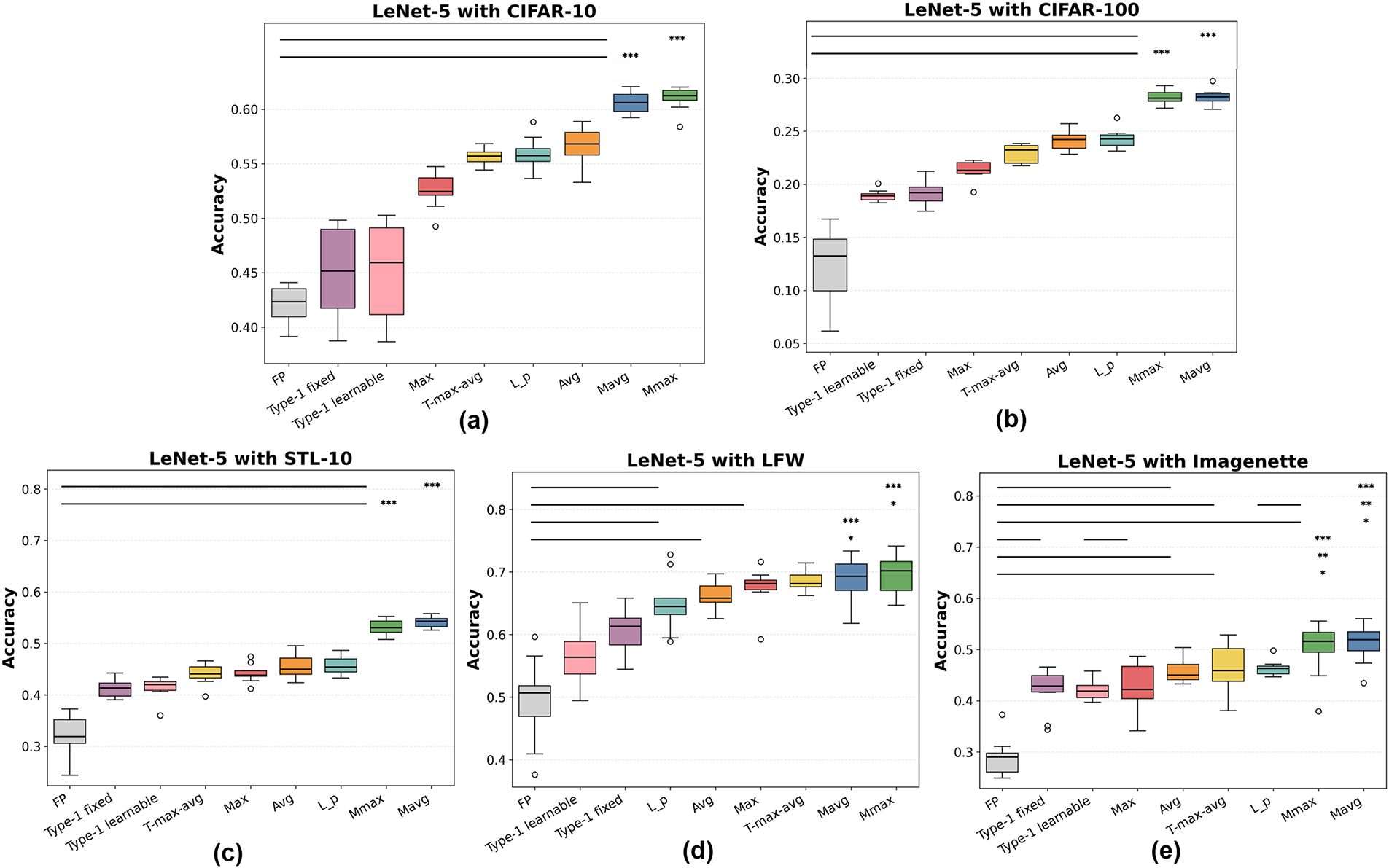
Figure 8: Classification accuracy of pooling methods with LeNet-5 on (a) CIFAR-10, (b) CIFAR-100, (c) STL-10, (d) LFW, and (e) Imagenette. FP denotes the fuzzy-pooling module in FP-CNN [37]. Horizontal bars with asterisks mark paired Wilcoxon signed-rank test results (∗:p<0.05, ∗∗:p<0.01, ∗∗∗:p<0.001) comparing the proposed fuzzy pooling (Mavg/Mmax) with the strongest non-membership baseline in each dataset

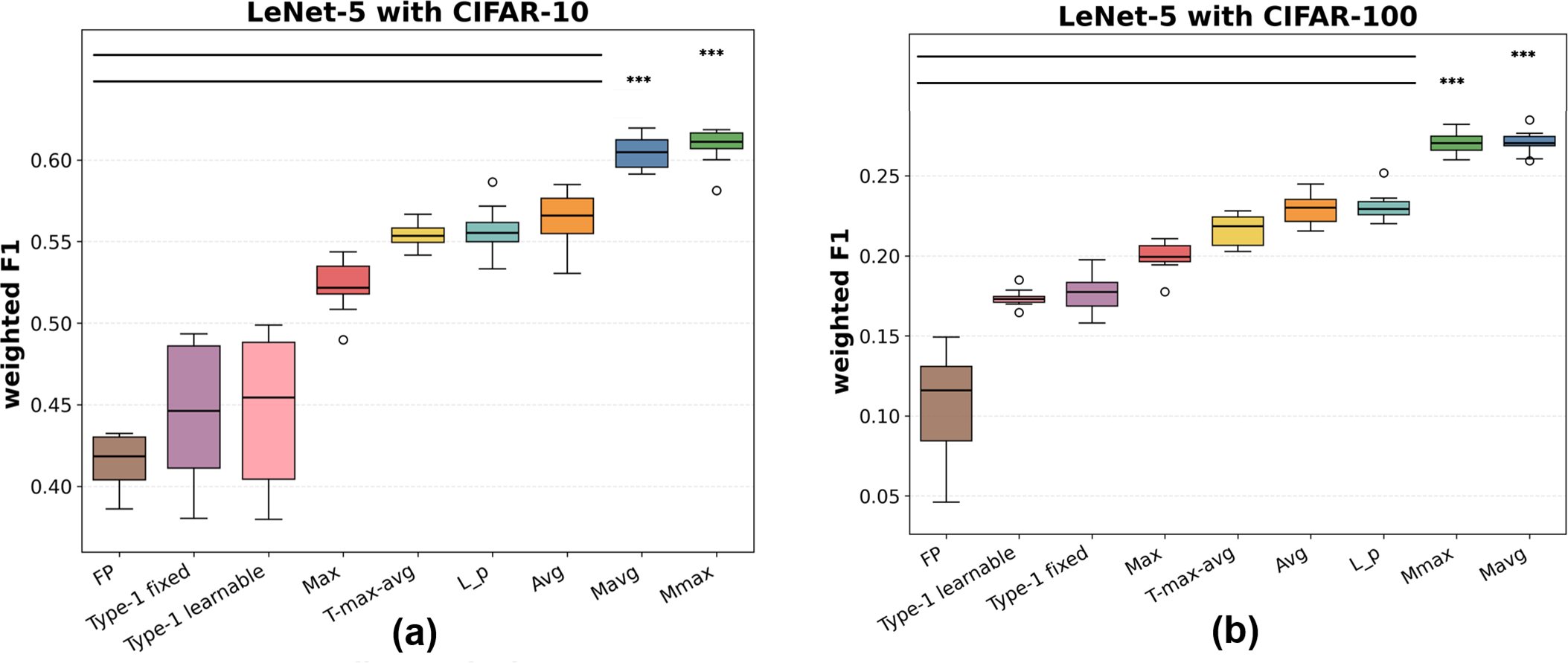
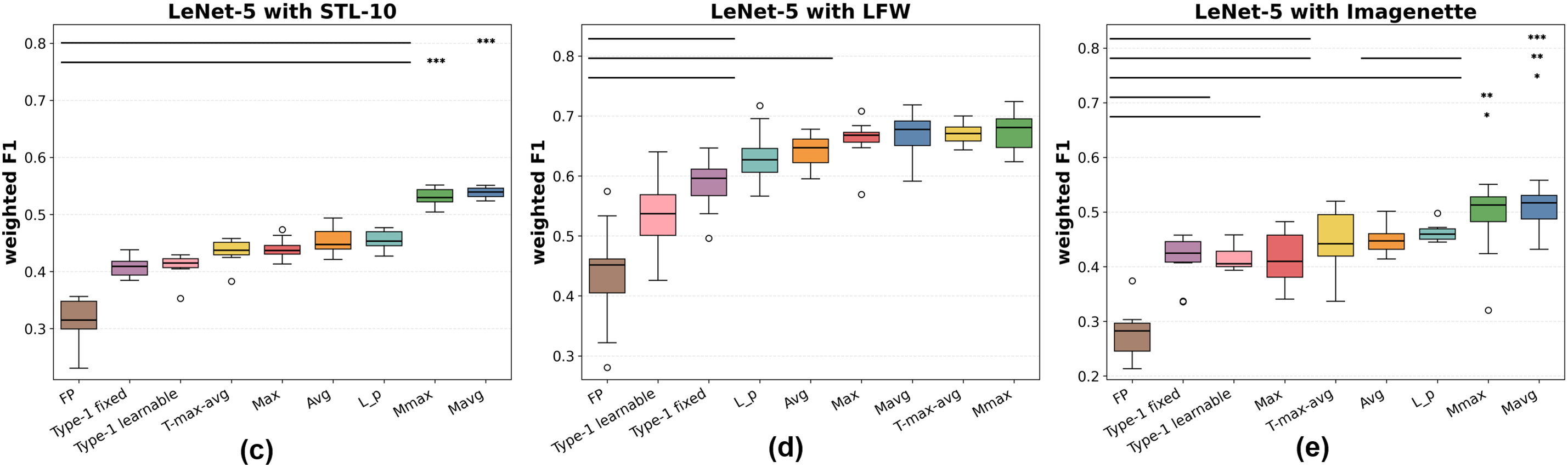
Figure 9: Weighted F1 scores of pooling methods with LeNet-5 on (a) CIFAR-10, (b) CIFAR-100, (c) STL-10, (d) LFW, and (e) Imagenette. Significance notation follows Fig. 8

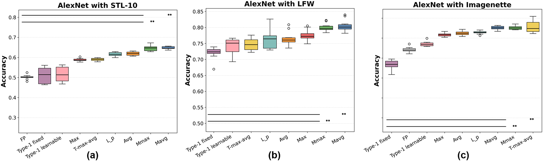
Figure 10: Classification accuracy of pooling methods with AlexNet on (a) STL-10, (b) LFW, and (c) Imagenette. FP denotes FP-CNN. Asterisks indicate significance under paired Wilcoxon tests (∗: p<0.05, ∗∗: p<0.01, ∗∗∗: p<0.001)

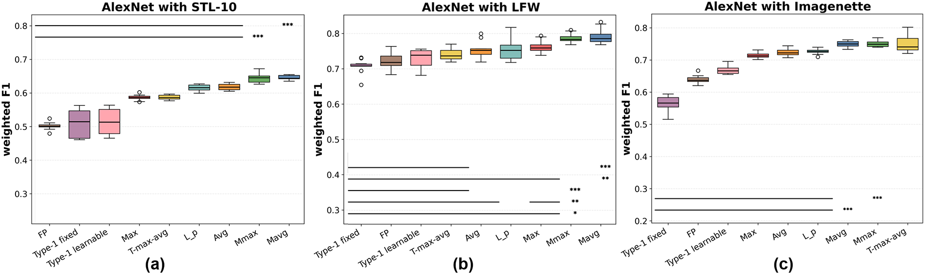
Figure 11: Weighted F1 scores of pooling methods with AlexNet on (a) STL-10, (b) LFW, and (c) Imagenette. Significance notation follows Fig. 10

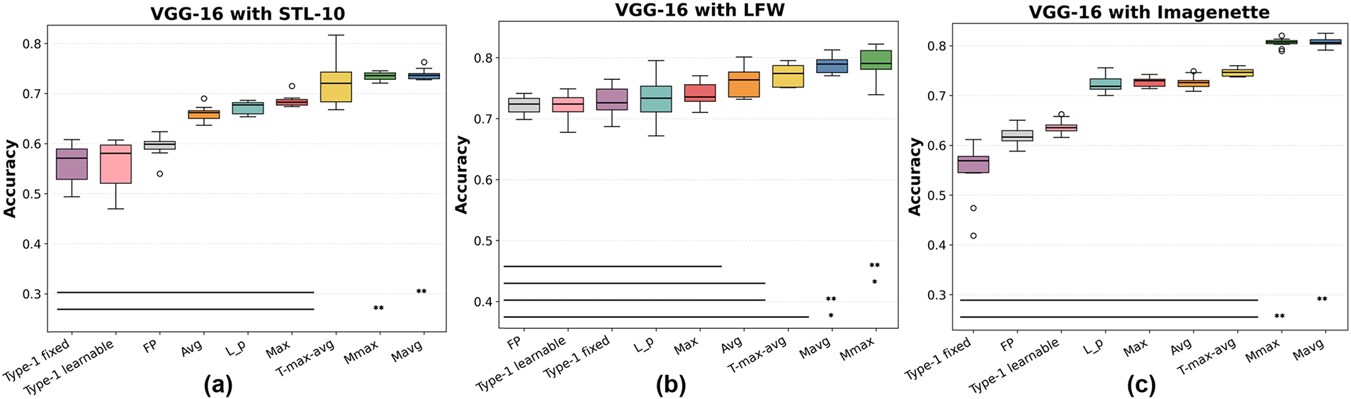
Figure 12: Classification accuracy of pooling methods with VGG-16 on (a) STL-10, (b) LFW, and (c) Imagenette. FP denotes FP-CNN. Significance bars follow the Wilcoxon test conventions in Fig. 8

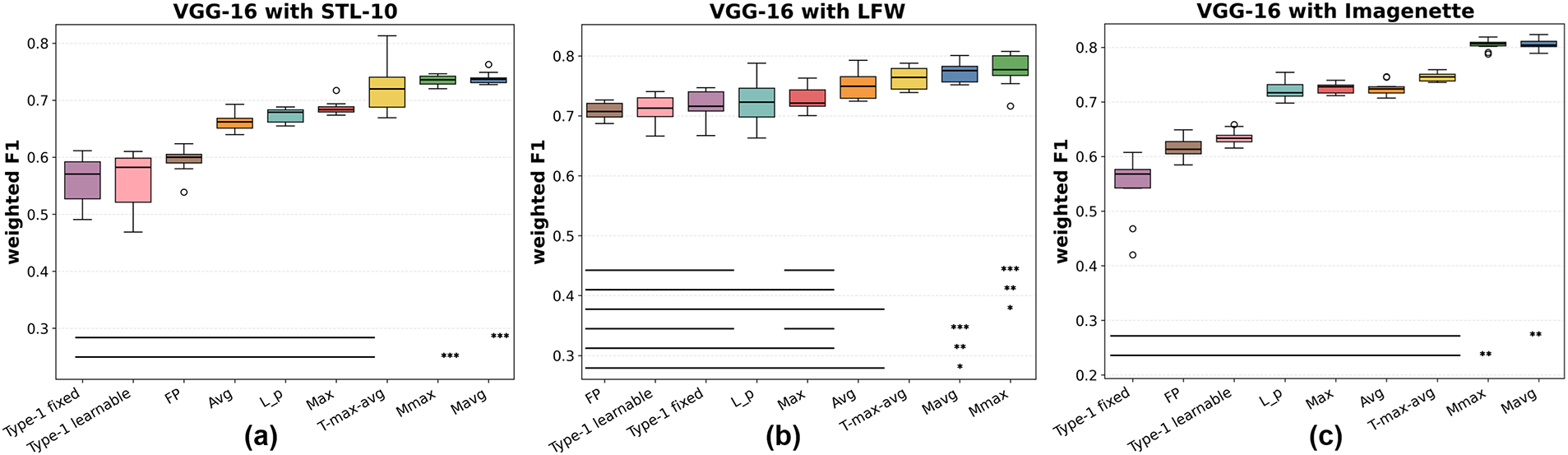
Figure 13: Weighted F1 scores of pooling methods with VGG-16 on (a) STL-10, (b) LFW, and (c) Imagenette. Significance notation follows Fig. 12

As detailed in Figs. 8 and 9, for LeNet-5, Mavg consistently outperforms Max, Avg, Lp, and T-max-avg on CIFAR-10 and CIFAR-100, with the gap particularly pronounced on CIFAR-100 given the higher class diversity. On STL-10, although the overall accuracy baseline is lower, both Mavg and Mmax retain the lead, while learnable Type-1 fuzzy and FP pooling show wider variance and unstable behavior. On LFW, Mavg attains the highest medians, though Lp and T-max-avg approach closely—suggesting that when class margins are subtle or inputs are structurally aligned, simpler pooling schemes can occasionally generalize competitively. On Imagenette, Mavg again dominates, achieving both the highest median and the tightest spread in accuracy and F1.

Referring to Figs. 10 and 11, for AlexNet, the superiority of Mavg and Mmax is also evident. On STL-10, Mmax performs best, closely followed by Mavg, both exhibiting small variance. On LFW, Lp or T-max-avg can sometimes match or slightly exceed the proposed methods, implying that under limited data and subtle inter-class separability, more complex pooling does not always guarantee gains over simpler adaptive baselines. In contrast, on Imagenette, both Mavg and Mmax clearly outperform the baselines, with significantly smaller variance across repeated runs.

As shown in Figs. 12 and 13, for VGG-16, the deeper backbone raises overall accuracy and F1 relative to LeNet-5 and AlexNet, yet Mavg consistently maintains a performance advantage—most visibly on LFW and Imagenette. While Lp and T-max-avg appear competitive in certain configurations, they exhibit wider variability and more outliers, whereas Mavg and Mmax offer stable and robust convergence.

Comparing accuracy and weighted F1 across all backbones, the relative rankings of pooling methods remain nearly identical. Weighted F1, which better accounts for class imbalance, further highlights the superiority of the proposed methods, especially on CIFAR-100 and Imagenette where the number of classes is large and intra-class variance is substantial. This indicates that membership-based pooling aggregates feature responses more effectively than either extremal selection (Max) or uniform averaging (Avg).

Statistical significance. To confirm that the observed performance gains are not due to random variation, paired two-sided Wilcoxon signed-rank tests were conducted over 10 independent runs per dataset and backbone. Horizontal bars and asterisks in Figs. 8–13 denote significance levels (∗:p<0.05, ∗∗:p<0.01, ∗∗∗:p<0.001). In nearly all cases, the proposed Mavg and Mmax achieve statistically significant improvements over both conventional (Avg, Max, Lp, T-max-avg) and fuzzy-type (Type-1, FP) pooling baselines, demonstrating that the observed advantages arise from the membership-based mechanism rather than random initialization.

In summary, Experiment 1 demonstrates that Mavg is the most consistently strong pooling method, with Mmax providing comparable or complementary benefits. Both converge reliably across diverse datasets and backbones, as evidenced by reduced variance and statistically significant improvements in most cases. While Lp or T-max-avg may serve as lightweight alternatives in constrained settings (e.g., LFW with AlexNet), membership-based pooling offers more robust and reproducible performance overall. Practically, Mavg is recommended as a default choice, whereas Mmax may be preferred when preserving high-frequency or edge-dominant features is critical, as qualitatively visualized in Appendix B.

Experiment 2 (Performance under limited supervision).

We investigate the impact of training-data scarcity by varying the fraction of training samples r∈{0.001,0.002,0.005,0.01,0.02,0.05,0.1,0.2,0.5} for LeNet-5 on MNIST and Fashion-MNIST. Figs. 14 and 15 summarize the trends in classification accuracy and weighted F1, respectively (reported as mean ± std over 5 converged HO runs).

Figure 14: Classification accuracy across training fractions for MNIST and Fashion-MNIST using LeNet-5 (Experiment 2). Shaded bands denote ±1 standard deviation over converged runs

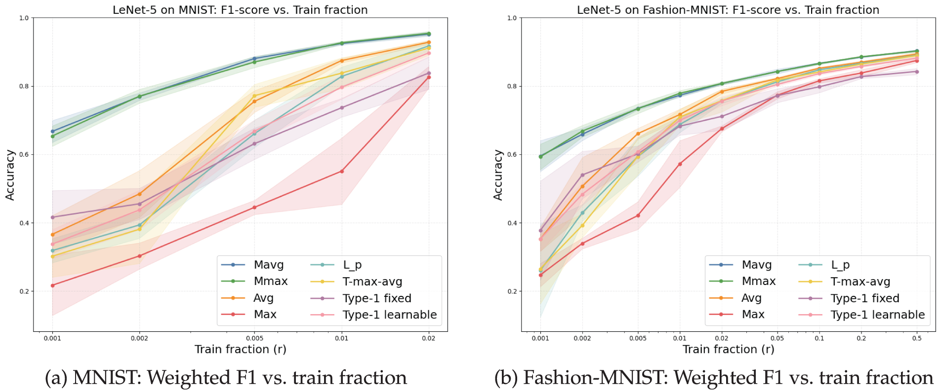
Figure 15: Weighted F1 across training fractions for MNIST and Fashion-MNIST using LeNet-5 (Experiment 2). Shaded bands denote ±1 standard deviation over converged runs

Overall, membership-based pooling (Mavg/Mmax) consistently outperforms conventional pooling operators on both datasets. On MNIST, the advantage is evident even at extremely small training ratios (r=0.001), where Mavg and Mmax sustain an accuracy >0.65 and weighted F1 >0.66, while Avg and Max fall below 0.40 on both metrics—indicating that the proposed pooling extracts salient features even under severe supervision constraints.

As r increases, all methods improve, but the relative ordering remains stable. Mavg and Mmax exceed 0.95 accuracy and 0.93 weighted F1 by r=0.02, whereas Avg and Max lag by a significant margin (>10 percentage points). Type-1 fuzzy baselines (fixed or learnable) improve over Avg/Max but exhibit high variance, especially at small r, signaling less stable convergence.

On Fashion-MNIST—which is more challenging due to higher intra-class variability—the gaps are even more pronounced at small fractions (r≤0.005): conventional pooling shows wider standard deviation bands and degraded F1, whereas Mavg and Mmax improve steadily with narrower uncertainty bands. As the training set grows (r≥0.05), all methods approach saturation, yet the proposed methods retain a notable edge, surpassing 0.90 weighted F1 at r=0.5.

Taken together, Experiment 2 validates the robustness of membership-based pooling under limited supervision, a common real-world scenario where large annotated datasets are unavailable. By aggregating responses via soft memberships—avoiding the pitfalls of both extremal selection (Max) and uniform averaging (Avg)—the proposed pooling family offers a stronger inductive bias that translates into superior generalization, particularly under data scarcity.

4.3 Analysis and Discussion

Key observations.

(1)  Across LeNet-5, AlexNet, and VGG-16, Mavg/Mmax typically achieve higher medians and tighter IQRs than Max/Avg/Lp/T-max-avg and both Type-1 fuzzy variants on CIFAR-100 and ImageNette, indicating simultaneous gains in accuracy and stability—critical when reproducibility matters.

(2)  On LFW, improvements are present but smaller. With AlexNet, conventional schemes may occasionally tie or slightly outperform the proposed layers. This suggests that when early features are already strongly structured (e.g., by large receptive fields or strong low-level inductive biases) and decision boundaries are subtle, pooling contributes less to overall discriminability.

(3)  Type-1 fuzzy pooling (fixed and learnable) consistently shows lower central tendency and higher variance. This aligns with the difficulty of specifying or stably learning crisp membership functions under noisy local statistics. By contrast, our FCM-style soft memberships adapt smoothly within each window, reducing sensitivity to local outliers and improving robustness—consistent with Experiment 2 results under limited supervision.

(4)  Weighted F1 mirrors accuracy across all settings, indicating that gains are not artifacts of class-frequency imbalance but reflect genuine improvements in balanced classification.

Overall implications.

Membership-based pooling provides a consistent inductive bias across architectures and datasets, particularly when data are noisy, imbalanced, or scarce. While its relative advantage can diminish under strongly regularized architectures or inherently separable feature spaces (e.g., LFW with AlexNet), the method remains robust and avoids the instability observed in Type-1 fuzzy baselines. These properties make it a practical drop-in replacement for standard pooling in real-world scenarios where dataset conditions are rarely ideal.

5  Conclusions

This work proposed two fuzzy C-means (FCM)-based pooling layers, Mavg (Membership-Averaging) and Mmax (Membership-Maxing), that bring soft, data-driven aggregation into convolutional neural networks. By leveraging fuzzy memberships computed per pooling region and converting them into a location-adaptive pooling exponent with BN-style stabilization (cf. Section 3), the layers preserve boundary ambiguity and reduce information loss typical of static operators (Max/Avg) while remaining drop-in compatible with standard CNNs.

Empirical findings.

Across Experiment 1 (three backbones: LeNet-5, AlexNet, VGG-16; five datasets: CIFAR-10/100, STL-10, LFW, ImageNette), membership-based pooling attained higher median accuracy and weighted F1 with tighter variability than Max/Avg/Lp/T-max-avg and Type-1 fuzzy baselines, with the largest gains on CIFAR-100 and ImageNette where class diversity and ambiguity are pronounced. In Experiment 2 (severe data scarcity on MNIST/Fashion-MNIST, down to r=0.001), Mavg/Mmax retained meaningful performance where conventional pooling degraded sharply—evidence that soft, membership-guided aggregation is robust in low-data regimes.

Limitations and scope.

Although the proposed fuzzy pooling layers are lightweight and drop-in compatible with existing CNNs, several limitations and considerations remain.

First, the computation of fuzzy memberships introduces a slight linear overhead proportional to the number of clusters K. This cost is small compared to convolutional operations and involves no iterative optimization. Importantly, unlike rule-based fuzzy systems or conditional pooling strategies, the proposed layer contains no branching operations, which preserves GPU pipelining efficiency and allows highly parallel execution across pooling regions. Consequently, inference speed remains close to that of conventional pooling, as verified in our complexity analysis (Section 3.7).

Second, the method’s performance shows moderate sensitivity to hyperparameters such as the number of clusters K and the fuzzifier m. Although stable results were obtained for K∈[2,9] and m=2.0 across datasets, further work could explore adaptive or data-driven tuning schemes to improve robustness across architectures and domains.

Third, the BN-style normalization effectively stabilizes training but assumes sufficiently large batch sizes for reliable statistics. When batch size is limited or streaming inference is required, alternatives such as Group Normalization or Instance Normalization may provide better stability while retaining the same integration principle.

Finally, our evaluations were based on publicly available image benchmarks to ensure comparability with prior pooling studies. While these datasets provide valuable diversity, future validation on real-world or domain-specific data—such as medical, environmental, or defense applications—would further demonstrate the method’s generalization and reliability under practical conditions.

Practical implications.

Mavg is a strong default due to its smoothness and stable convergence; Mmax can be preferable when preserving high-frequency or edge-dominant responses is critical. Using K close to the number of classes worked reliably across settings, and BN-style post-normalization consistently improved training stability and reproducibility. That said, benefits diminish when early features are already highly separable (e.g., AlexNet on LFW), suggesting that architecture capacity and dataset characteristics should inform the choice of variant and K.

Future work.

•   Hyperparameters and rules. Systematic study of K, fuzzifier m, and exponent-composition rules (e.g., temperature-controlled averaging, entropy-aware mixing) to balance accuracy and efficiency.

•   Learning strategies. Regularization/scheduling for the membership map, bilevel objectives for centroids vs. features, and calibration-aware training to improve reliability under shift.

•   Architectural/generalization breadth. Extending to modern backbones (ResNets, ConvNeXts, Transformers) and tasks beyond classification (detection/segmentation), including dense prediction where spatial ambiguity is critical.

•   Coupled optimization. Joint refinement of memberships and features (e.g., alternating updates, meta-learning of pk and m), and exploring probabilistic or mixture-of-experts views that unify clustering and pooling.

Summary.

Embedding fuzzy memberships into pooling offers a principled and practical path to more robust, generalizable CNNs. By consistently improving accuracy and balanced metrics across architectures, datasets, and supervision levels—and by retaining a simple drop-in form—Mavg/Mmax illustrate the value of importing fuzzy-set principles into core deep learning operators.

Acknowledgement: The authors would like to express their gratitude to all collaborators who provided constructive feedback during this study.

Funding Statement: This research was supported by the Institute of Information & Communications Technology Planning & Evaluation (IITP)–ITRC (Information Technology Research Center) grant funded by the Korea government (MSIT) (IITP-2025-RS-2023-00260098, 50%), and the Aerospace and ICT Localization & Commercialization Technology Development Project funded by Gyeongsangnam-do and the Gyeongnam Techno park (50%).

Author Contributions: Conceptualization, Seunggyu Byeon, Jung-hun Lee and Jong-Deok Kim; methodology, Seunggyu Byeon; software, Seunggyu Byeon; validation, Seunggyu Byeon and Jung-hun Lee; formal analysis, Seunggyu Byeon; investigation, Seunggyu Byeon and Jung-hun Lee; writing—original draft preparation, Seunggyu Byeon; writing—review and editing, Seunggyu Byeon and Jong-Deok Kim; visualization, Seunggyu Byeon and Jung-hun Lee; supervision, Jong-Deok Kim; project administration, Jong-Deok Kim; funding acquisition, Jong-Deok Kim. All authors reviewed the results and approved the final version of the manuscript.

Availability of Data and Materials: All datasets used in this study are publicly available: CIFAR-10/100, STL-10, LFW (subset), ImageNette, MNIST, and Fashion-MNIST (see Tables 2 and 3). The implementation of the proposed Mavg/Mmax pooling layers (including training and evaluation scripts) is available at: https://colab.research.google.com/drive/1u8S6Nyp8Ojciy28bMGnZXIoYuehoADCJ?usp=sharing. If any access issues occur, please contact the corresponding author.

Ethics Approval: Not applicable.

Conflicts of Interest: The authors declare no conflicts of interest to report regarding the present study.

Abbreviations

Appendix A Ablation Results on BN-Style Normalization

This appendix summarizes the detailed ablation results for BN-style normalization applied after the proposed fuzzy pooling layer. The normalization follows the standard batch normalization formulation described in [31]. The quantitative comparisons across datasets and backbones are presented in Table A1.

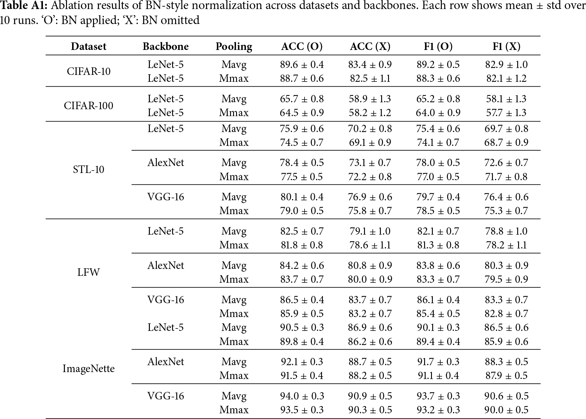
CIFAR-10 and CIFAR-100 were evaluated using LeNet-5, while STL-10, LFW, and ImageNette were tested on LeNet-5, AlexNet, and VGG-16 backbones. Each row reports the mean ± standard deviation over 10 converged runs for classification accuracy and weighted F1 score. ‘O’ indicates that BN is applied, and ‘X’ denotes that BN is omitted. All experiments used a batch size of 32 to ensure reliable statistics.

BN consistently improves both accuracy and weighted F1 across all datasets. As shown in Table A1, for simpler networks such as LeNet-5 (CIFAR-10/100), the improvement reaches up to 7%–8% absolute, while for deeper networks (AlexNet, VGG-16) on larger datasets, BN contributes steady 3%–5% gains with reduced variance. These results confirm that BN acts as a structural stabilizer against fluctuations induced by fuzzy memberships and adaptive pooling exponents.

Appendix B Visualization of the Proposed Fuzzy Pooling Layer

To provide a qualitative understanding of how the proposed fuzzy pooling operates, we visualize intermediate feature maps and the final pooled responses under different settings. The visualization clarifies how the clustering process, learned pooling exponents, and cluster integration—as detailed in Section 3—jointly determine the spatial saliency pattern produced by the layer.

In all cases, the process proceeds in four stages:

(i)   Fuzzy clustering: local features are grouped into K latent types via FCM [28];

(ii)  Cluster-wise feature mapping: each cluster yields a distinct feature response map;

(iii) Adaptive modulation: learned exponents pk emphasize or suppress clusters according to local memberships;

(iv)  Integration: the maps are merged using either Membership Averaging (Mavg) or Membership Maxing (Mmax).

Fig. A1a,b illustrates the effect of learned pooling exponents when p=[5,0.2,0.2] for three clusters. Because memberships ub,ij,k∈[0,1] act as continuous weights, values of pk>1 attenuate activation magnitudes (suppressing those regions), whereas pk<1 amplify salient responses. In this example, the two clusters with smaller pk values (0.2) produce enhanced contrast—appearing brighter or darker—while the cluster with pk=5 becomes subdued. This contrast amplification yields visually sharper spatial boundaries, consistent with the adaptive nature of the proposed pooling described in Section 3.6.

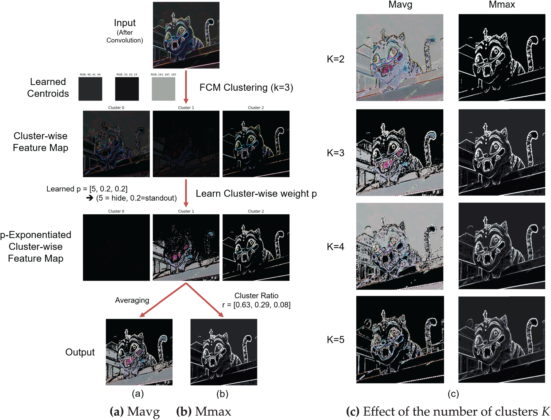
Figure A1: Visual comparison of the proposed fuzzy pooling layer. (a,b) show two integration variants derived from identical fuzzy memberships: both start from the same clustering and per-cluster feature maps, modulate local saliency using learned exponents pk (p=[5,0.2,0.2] in this example), and integrate responses by either soft averaging (Mavg) or dominance-based maxing (Mmax). Clusters with pk<1 amplify features (bright or dark contrast), while pk>1 suppress them, leading to clearer spatial delineation. (c) illustrates how the number of clusters K affects selectivity: as K increases, finer semantic regions appear, with K=3 showing the most pronounced separation where two clusters are enhanced and one is attenuated

These qualitative results demonstrate that the proposed fuzzy pooling not only blends average and max pooling behaviors but also adaptively modulates feature intensity through the learned exponents pk. This produces locally contrast-enhanced feature representations, helping subsequent layers distinguish boundary and texture information more effectively under varying fuzzy memberships.

References

1. Lecun Y, Bottou L, Bengio Y, Haffner P. Gradient-based learning applied to document recognition. Proc IEEE. 1998;86(11):2278–324. doi:10.1109/5.726791. [Google Scholar] [CrossRef]

2. Krizhevsky A, Sutskever I, Hinton GE. Imagenet classification with deep convolutional neural networks. In: Advances in Neural Information Processing Systems. Vol. 25. Late Tahoe, NV, USA: Neuro IPS; 2012. [Google Scholar]

3. Hendrycks D, Dietterich T. Benchmarking neural network robustness to common corruptions and perturbations. arXiv:1903.12261. 2019. [Google Scholar]

4. Guo C, Pleiss G, Sun Y, Weinberger KQ. On calibration of modern neural networks. In: Proceedings of the 34th International Conference on Machine Learning; 2017 Aug 6–11; Sydney, NSW, Australia. New Orleans, LA, USA: PMLR; 2017. p. 1321–30. [Google Scholar]

5. Minderer M, Djolonga J, Romijnders R, Hubis F, Zhai X, Houlsby N, et al. Revisiting the calibration of modern neural networks. Adv Neural Inform Process Syst. 2021;34:15682–94. [Google Scholar]

6. Ovadia Y, Fertig E, Ren J, Nado Z, Sculley D, Nowozin S, et al. Can you trust your model’s uncertainty? Evaluating predictive uncertainty under dataset shift. In: Advances in neural information processing systems. Vol. 32. Vancouver, BC, Canada: Neuro IPS; 2019. [Google Scholar]

7. Zafar A, Aamir M, Mohd Nawi N, Arshad A, Riaz S, Alruban A, et al. A comparison of pooling methods for convolutional neural networks. Appl Sci. 2022;12(17):8643. doi:10.3390/app12178643. [Google Scholar] [CrossRef]

8. Rippel O, Snoek J, Adams RP. Spectral representations for convolutional neural networks. In: Advances in neural information processing systems. Vol. 28. Montreal, QC, Canada: Neuro IPS; 2015. [Google Scholar]

9. Simonyan K, Zisserman A. Very deep convolutional networks for large-scale image recognition. arXiv:1409.1556. 2014. [Google Scholar]

10. Lin M, Chen Q, Yan S. Network in network. arXiv:1312.4400. 2013. [Google Scholar]

11. Szegedy C, Liu W, Jia Y, Sermanet P, Reed S, Anguelov D, et al. Going deeper with convolutions. In: Proceedings of the IEEE Conference on Computer Vision and Pattern Recognition; 2015 Jun 7–12; Boston, MA, USA. p. 1–9. doi:10.1109/CVPR.2015.7298594. [Google Scholar] [CrossRef]

12. Szegedy C, Vanhoucke V, Ioffe S, Shlens J, Wojna Z. Rethinking the inception architecture for computer vision. In: Proceedings of the 2016 IEEE Conference on Computer Vision and Pattern Recognition (CVPR); 2016 Jun 27–30; Las Vegas, NV, USA. p. 2818–26. doi:10.1109/CVPR.2016.308. [Google Scholar] [CrossRef]

13. Szegedy C, Ioffe S, Vanhoucke V, Alemi A. Inception-v4, inception-resnet and the impact of residual connections on learning. In: Proceedings of the AAAI Conference on Artificial Intelligence; 2017 Feb 11; San Francisco, CA, USA. Vol. 31. p. 4278–84. doi:10.1609/aaai.v31i1.11231. [Google Scholar] [CrossRef]

14. Springenberg JT, Dosovitskiy A, Brox T, Riedmiller M. Striving for simplicity: the all convolutional net. arXiv:1412.6806. 2014. [Google Scholar]

15. He K, Zhang X, Ren S, Sun J. Deep residual learning for image recognition. In: Proceedings of the IEEE Conference on Computer Vision and Pattern Recognition; 2016 Jun 27–30; Las Vegas, NV, USA. p. 770–8. doi:10.1109/CVPR.2016.90. [Google Scholar] [CrossRef]

16. Tan M, Le Q. Efficientnet: rethinking model scaling for convolutional neural networks. In: International Conference on Machine Learning; 2019 Jun 9–15; Long Beach, CA, USA. p. 6105–14. [Google Scholar]

17. Hu J, Shen L, Sun G. Squeeze-and-excitation networks. In: Proceedings of the IEEE Conference on Computer Vision and Pattern Recognition; 2018 Jun 18–23; Salt Lake City, UT, USA. p. 7132–41. doi:10.1109/CVPR.2018.00745. [Google Scholar] [CrossRef]

18. Woo S, Park J, Lee JY, Kweon IS. Cbam: convolutional block attention module. In: Proceedings of the European Conference on Computer Vision. Munich, Germany: ECCV; 2018. p. 3–19. [Google Scholar]

19. Liu Z, Mao H, Wu CY, Feichtenhofer C, Darrell T, Xie S. A convnet for the 2020s. In: Proceedings of the IEEE/CVF Conference on Computer Vision and Pattern Recognition; 2022 Jun 18–24; New Orleans, LA, USA. p. 11976–86. doi:10.1109/CVPR52688.2022.01167. [Google Scholar] [CrossRef]

20. Dosovitskiy A. An image is worth 16x16 words: transformers for image recognition at scale. arXiv: 2010.11929. 2020. [Google Scholar]

21. Gulcehre C, Cho K, Pascanu R, Bengio Y. Learned-norm pooling for deep feedforward and recurrent neural networks. In: Joint European Conference on Machine Learning and Knowledge Discovery in Databases. Nancy, France: Berlin/Heidelberg, Germany: Springer; 2014. p. 530–46. doi:10.1007/978-3-662-44848-9_34. [Google Scholar] [CrossRef]

22. Bieder F, Sandkühler R, Cattin P. Comparison of methods generalizing max-and average-pooling. arXiv:2103.01746. 2021. [Google Scholar]

23. Radenović F, Tolias G, Chum O. Fine-tuning CNN image retrieval with no human annotation. IEEE Trans Pattern Anal Mach Intell. 2018;41(7):1655–68. doi:10.1109/TPAMI.2018.2846566. [Google Scholar] [PubMed] [CrossRef]

24. Zeiler MD, Fergus R. Stochastic pooling for regularization of deep convolutional neural networks. arXiv:1301.3557. 2013. [Google Scholar]

25. Zhai S, Wu H, Kumar A, Cheng Y, Lu Y, Zhang Z, et al. S3pool: pooling with stochastic spatial sampling. In: Proceedings of the IEEE Conference on Computer Vision and Pattern Recognition; 2017 Jul 21–26; Honolulu, HI, USA. p. 4970–8. [Google Scholar]

26. Zadeh LA. Fuzzy sets. Inform Control. 1965;8(3):338–53. doi:10.1016/S0019-9958(65)90241-X. [Google Scholar] [CrossRef]

27. Dunn JC. A fuzzy relative of the ISODATA process and its use in detecting compact well-separated clusters. J Cybern. 1973;3(3):32–57. doi:10.1080/01969727308546046. [Google Scholar] [CrossRef]

28. Bezdek JC. Pattern recognition with fuzzy objective function algorithms. New York, NY, USA: Berlin/Heidelberg, Germany: Springer; 1981. [Google Scholar]

29. Goodfellow I. Deep learning. Cambridge, MA, USA: MIT press; 2016. [Google Scholar]

30. Zhang R. Making convolutional networks shift-invariant again. In: International Conference on Machine Learning. Long Beach, CA, USA: PMLR; 2019. p. 7324–34. [Google Scholar]

31. Ioffe S, Szegedy C. Batch normalization: accelerating deep network training by reducing internal covariate shift. In: Proceedings of the 32nd International Conference on Machine Learning; 2015 Jul 7–9; Lille, France. p . 448–56. [Google Scholar]

32. Santurkar S, Tsipras D, Ilyas A, Madry A. How does batch normalization help optimization? In: Bengio S, Wallach H, Larochelle H, Grauman K, Cesa-Bianchi N, Garnett R, editors. Advances in Neural Information Processing Systems. Vol. 31. Montréal, QC, Canada: Neuro IPS; 2018. [Google Scholar]

33. Zhao L, Zhang Z. A improved pooling method for convolutional neural networks. Sci Rep. 2024;14(1):1589. [Google Scholar] [PubMed]

34. Sharma T, Singh V, Sudhakaran S, Verma NK. Fuzzy based pooling in convolutional neural network for image classification. In: Proceedings of the 2019 IEEE International Conference on Fuzzy Systems; 2019 Jun 23–26; New Orleans, LA, USA. p. 1–6. doi:10.1109/FUZZ-IEEE.2019.8859010. [Google Scholar] [CrossRef]

35. Diamantis DE, Iakovidis DK. Fuzzy pooling. IEEE Trans Fuzzy Syst. 2020;29(11):3481–8. doi:10.1109/TFUZZ.2020.3024023. [Google Scholar] [CrossRef]

36. Wang Y, Wang Y, Er MJ, Zhu J. Unsupervised fuzzy neural network for image clustering. In: Proceedings of the 2021 IEEE International Conference on Fuzzy Systems; 2021 Jul 11–14; Luxembourg. p. 1–6. doi:10.1109/FUZZ45933.2021.9494601. [Google Scholar] [CrossRef]

37. Hasan MM, Hossain MM, Rahman MM, Azad A, Alyami SA, Moni MA. FP-CNN: a fuzzy pooling-based convolutional neural network for medical image classification. Comput Biol Med. 2023;166(3):107407. doi:10.1016/j.compbiomed.2023.107407. [Google Scholar] [CrossRef]

38. Lin CJ, Chen BH, Lin CH, Jhang JY. Design of a convolutional neural network with Type-2 fuzzy-based pooling for vehicle recognition. Mathematics. 2024;12(24):3885. doi:10.3390/math12243885. [Google Scholar] [CrossRef]

39. Thakur PS, Verma RK, Tiwari R. Analysis of time complexity of K-means and fuzzy C-means clustering algorithm. Eng Math Lett. 2024;2024(4). doi:10.28919/eml/8402. [Google Scholar] [CrossRef]

40. Krizhevsky A. Learning multiple layers of features from tiny images. Toronto, ON, Canada: University of Toronto; 2009. [Google Scholar]

41. Huang GB, Mattar M, Berg T, Learned-Miller E. Labeled faces in the wild: a database forstudying face recognition in unconstrained environments. In: Workshop on Faces in ‘Real-Life’ Images: Detection, Alignment, and Recognition. Marseille, France: HAL; 2008. [Google Scholar]

42. Coates A, Ng A, Lee H. An analysis of single-layer networks in unsupervised feature learning. In: Proceedings of the Fourteenth International Conference on Artificial Intelligence and Statistics; 2011 Apr 11–13; Fort Lauderdale, FL, USA. p. 215–23. [Google Scholar]

43. Deng J, Dong W, Socher R, Li LJ, Li K, Fei-Fei L. Imagenet: a large-scale hierarchical image database. In: Proceedings of the 2009 IEEE Conference on Computer Vision and Pattern Recognition; 2009 Jun 20–25; Miami, FL, USA. p. 248–55. doi:10.1109/CVPR.2009.5206848. [Google Scholar] [CrossRef]

44. Xiao H, Rasul K, Vollgraf R. Fashion-mnist: a novel image dataset for benchmarking machine learning algorithms. arXiv:1708.07747. 2017. [Google Scholar]