Hierarchical Attention Transformer for Multivariate Time Series Forecasting

1  Introduction

Time series data is widely used in modern systems, from monitoring sensor readings in industrial equipment to analyzing market trends in finance. These sequences often exhibit patterns that vary over time, influenced by factors such as seasonality, trends, and sudden events. Accurate forecasting of such data enables proactive decision-making, optimizing resource allocation and mitigating risks in real-world applications. However, the inherent multi-scale nature of time series where short-term variations interact with longer-term cycles poses significant challenges for traditional modeling approaches.

In particular, multivariate time series forecasting is fundamental to decision-making across critical infrastructure systems. In electrical grid management, operators must simultaneously monitor 15-min load fluctuations for immediate balancing while tracking daily and seasonal patterns for capacity planning [1,2]. Transportation networks require real-time traffic flow prediction alongside weekly commuting pattern analysis for optimal routing. Financial markets demand millisecond price movement forecasting integrated with long-term trend analysis. These applications share a common challenge: temporal patterns manifest across multiple scales with complex interdependencies that current forecasting methods inadequately capture.

Transformer architectures have shown promising results in time series forecasting, building on their success in sequence modeling [3]. Recent innovations include Informer’s sparse attention for computational efficiency [4], Autoformer’s decomposition-based approach [5], and iTransformer’s variable-centric tokenization strategy [6]. However, these methods primarily operate at single temporal resolutions, processing sequences uniformly without explicitly modeling the multi-scale nature of temporal data.

Multi-scale approaches recognize temporal heterogeneity but face fundamental limitations. Methods like Pyraformer employ separate parameters for each scale [7], while Scaleformer processes scales independently [8]. TimesNet transforms sequences to frequency domain for multi-period analysis [9]. These approaches capture patterns at different temporal granularities but lack mechanisms for cross-scale information exchange, missing critical dependencies where short-term fluctuations are influenced by long-term trends and vice versa.

Consider electricity load forecasting where immediate demand spikes (captured at 15-min resolution) are strongly influenced by daily usage patterns and seasonal trends (requiring hourly to weekly analysis). Current methods process these scales separately, failing to model how weekend-to-weekday transitions affect intraday variations or how seasonal changes modify daily peak patterns. This limitation becomes critical during demand transitions, where cross-scale interactions determine prediction accuracy.

We propose HAT (Hierarchical Attention Transformer) to address these challenges through three key innovations. First, we develop a cross-scale attention mechanism that enables direct information exchange between temporal hierarchies through unified attention frameworks, allowing fine-grained patterns to inform long-term predictions and seasonal trends to guide short-term forecasting. Second, we design Hierarchical Attention Embedding (HAE) that combines convolutional feature extraction with recurrent temporal modeling at multiple window sizes, creating compact multi-scale representations suitable for Transformer processing. Third, we implement gradient flow optimization through residual connections and skip paths across scales, ensuring stable training in deep hierarchical networks while maintaining computational efficiency.

The cross-scale attention mechanism represents our key contribution and a conceptual extension beyond prior multi-scale architectures. Unlike Pyraformer, which utilizes a rigid pyramidal attention mask that restricts information flow to neighboring parent-child scales, HAT treats temporal scales as global tokens in a unified attention space [7]. This allows the highest-level trend (e.g., weekly seasonality) to attend directly to fine-grained details (e.g., instantaneous spikes) in a single hop (O(1) path length), rather than propagating through intermediate layers.

Also, unlike Scaleformer, which refines scales iteratively, HAT fuses multi-resolution representations simultaneously via a learnable temperature-controlled mechanism, preserving both global context and local anomalies [8].

Our main contributions are summarized as follows:

•   Unified Cross-Scale Attention: Unlike Pyraformer (which uses separate parameters per scale) and Scaleformer (which processes different scales independently), HAT introduces a unified attention mechanism that allows direct information exchange between different temporal resolutions, enabling long-term trends (e.g., weekly patterns) to directly attend to short-term dynamics (e.g., hourly fluctuations).

•   Gradient Flow Optimization: We propose a hierarchical design using residual connections and skip paths across multiple temporal levels, which effectively alleviates the gradient vanishing problem commonly observed in deep multi-scale temporal architectures.

•   Efficiency Performance: We demonstrate that HAT achieves highly competitive forecasting accuracy while being 6.1× faster to train than leading patch-based methods (e.g., PatchTST), benefiting from the proposed hierarchical downsampling and fusion strategy.

2  Related Work

2.1 Transformer-Based Time Series Forecasting

The adaptation of Transformers to time series has yielded continuous improvements through architectural innovations. Informer introduced ProbSparse self-attention to reduce computational complexity [4], while Autoformer incorporated decomposition and auto-correlation mechanisms [5]. iTransformer proposed treating individual series as tokens rather than time steps [6]. FEDformer enhanced modeling through frequency domain analysis [10], and PatchTST introduced patching strategies treating subseries as tokens [11]. Recent efficiency improvements include linear attention mechanisms [12] and memory-efficient attention computation through Flash Attention [13]. However, these methods primarily operate at single temporal resolutions, limiting their ability to capture multi-scale patterns.

2.2 Multi-Scale Time Series Analysis

Multi-scale approaches recognize the importance of capturing patterns across different temporal granularities. Classical methods like STL and MSTL provide decomposition frameworks [14]. Pyraformer introduced pyramidal attention for multi-scale dependencies but employs separate parameters per scale [7]. Scaleformer proposed iterative multi-scale refinement through independent scale processing [8]. Recent work includes multiscale patch-wise modeling [15] and adaptive pathway selection [16]. Recent studies have also explored frequency-domain modeling for long-term time series forecasting. In particular, the Frequency–Wavelet Adaptive Basis Network (FWABN) leverages a wavelet–frequency hybrid representation to capture multi-resolution temporal patterns in the spectral domain. By adaptively learning basis functions across different frequency bands, such methods demonstrate strong capability in modeling periodicity and long-range dependencies. Unlike these frequency-domain approaches, our proposed HAT explicitly models cross-scale temporal interactions in the time domain through hierarchical embeddings and unified attention fusion, providing a complementary and more interpretable perspective on multi-scale dependency modeling [17].

WaveNet demonstrated the effectiveness of dilated convolutions for multi-scale temporal modeling [18]. TCN extended temporal convolutional approaches with residual connections [19]. N-HiTS proposed hierarchical interpolation for multi-horizon forecasting [20]. TimesNet introduced TimesBlock for multi-period analysis [9]. However, these approaches lack unified cross-scale attention mechanisms for effective information exchange.

2.3 Hierarchical and Cross-Scale Mechanisms

Hierarchical approaches have demonstrated promise for capturing dependencies across temporal levels. Chung et al. [21] introduced hierarchical multiscale RNNs with clock-based mechanisms. TimeMixer proposed decomposable multiscale mixing but lacks direct cross-scale attention [22]. Recent work on hierarchical spatio-temporal attention demonstrates the potential of attention mechanisms across hierarchical structures [23], though primarily for spatio-temporal rather than purely temporal forecasting. Feature Pyramid Networks established principles for hierarchical feature fusion across scales [23], while U-Net architectures demonstrated effective skip connections in hierarchical processing [24]. CrossFormer addressed cross-dimensional dependencies through two-stage attention mechanisms [25].

2.4 Gradient Flow Optimization

Training deep temporal networks faces challenges in gradient flow across multiple scales. Residual connections have become standard for stabilizing training in deep architectures [26], while DenseNet introduced dense connectivity patterns for improved gradient flow [27]. Layer normalization addresses internal covariate shift [28]. RevIN specifically addressed distribution shift in time series through reversible instance normalization [29]. Highway networks introduced gating mechanisms for deep network training [30]. However, optimizing gradient flow in hierarchical temporal architectures with cross-scale attention mechanisms remains underexplored, motivating our gradient flow optimization approach in HAT.

2.5 Summary and Research Gap

While the literature has advanced significantly from basic statistical methods to complex Transformers, a critical gap remains in the treatment of temporal scales. Existing multi-scale approaches (e.g., Pyraformer, Scaleformer) largely process hierarchies in isolation or through rigid bottom-up pathways. They lack a mechanism for direct attention between a high-level trend token and a low-level detail token. This limitation prevents models from dynamically adjusting short-term predictions based on global context in a single computational step. HAT addresses this specific gap by introducing a unified attention space where all temporal scales coexist, enabling O(1) path length for information flow across hierarchies.

3  Methodology

3.1 Problem Formulation

Given a multivariate time series X∈RB×L×N, where B is the batch size, L is the lookback window length, and N is the number of variables, the goal is to forecast the future horizon Y^∈RB×H×N for prediction length H. Each timestep xt∈RN contains synchronized observations across all variables.

The core challenge arises from temporal patterns that emerge simultaneously at multiple resolutions e.g., high-frequency fluctuations (15-min load spikes), medium-term cycles (daily routines), and long-term trends (weekly/seasonal effects). These scales are deeply interdependent: short-term anomalies are modulated by daily patterns, which in turn are shaped by seasonal shifts. Standard single-scale Transformers cannot capture such cross-scale dynamics.

3.2 Overall Architecture

The Hierarchical Attention Transformer (HAT) follows an encoder-only design with four core stages:

1.   RevIN [29] for distribution stabilization,

2.   Hierarchical Attention Embedding (HAE) with cross-scale interaction,

3.   Standard Transformer Encoder operating on variable-centric tokens,

4.   Linear Projection to horizon H followed by denormalization.

The forward pass is defined as

Xnorm,frev=RevIN⁡(X)∈RB×L×N,(1)

E=HAE⁡(Xnorm,Xmark)∈RB×N×dmodel,(2)

E′=Encoder⁡(E)∈RB×N×dmodel,(3)

Y^=frev(Linear⁡(E′))∈RB×H×N,(4)

where Xmark∈RB×L×C denotes optional timestamp embeddings (e.g., hour-of-day, day-of-week), and the final linear layer maps the embedding dimension dmodel to the prediction length H along the temporal axis. The full pipeline is illustrated in Fig. 1.

Figure 1: Complete architecture of the Hierarchical Attention Transformer (HAT). Input passes through RevIN → HAE (multi-scale conv-GRU + cross-scale attention) → Transformer encoder → horizon projection → RevIN denormalization.

3.3 Hierarchical Attention Embedding (HAE)

The HAE module serves as the encoder embedding layer. It is designed to extract multi-scale features by processing the input time series as independent univariate channels before fusing them. The process involves three stages: Hierarchical Convolutional–Recurrent Extraction, Gradient Flow Optimization, and Cross-Scale Attention, as illustrated in Fig. 2.

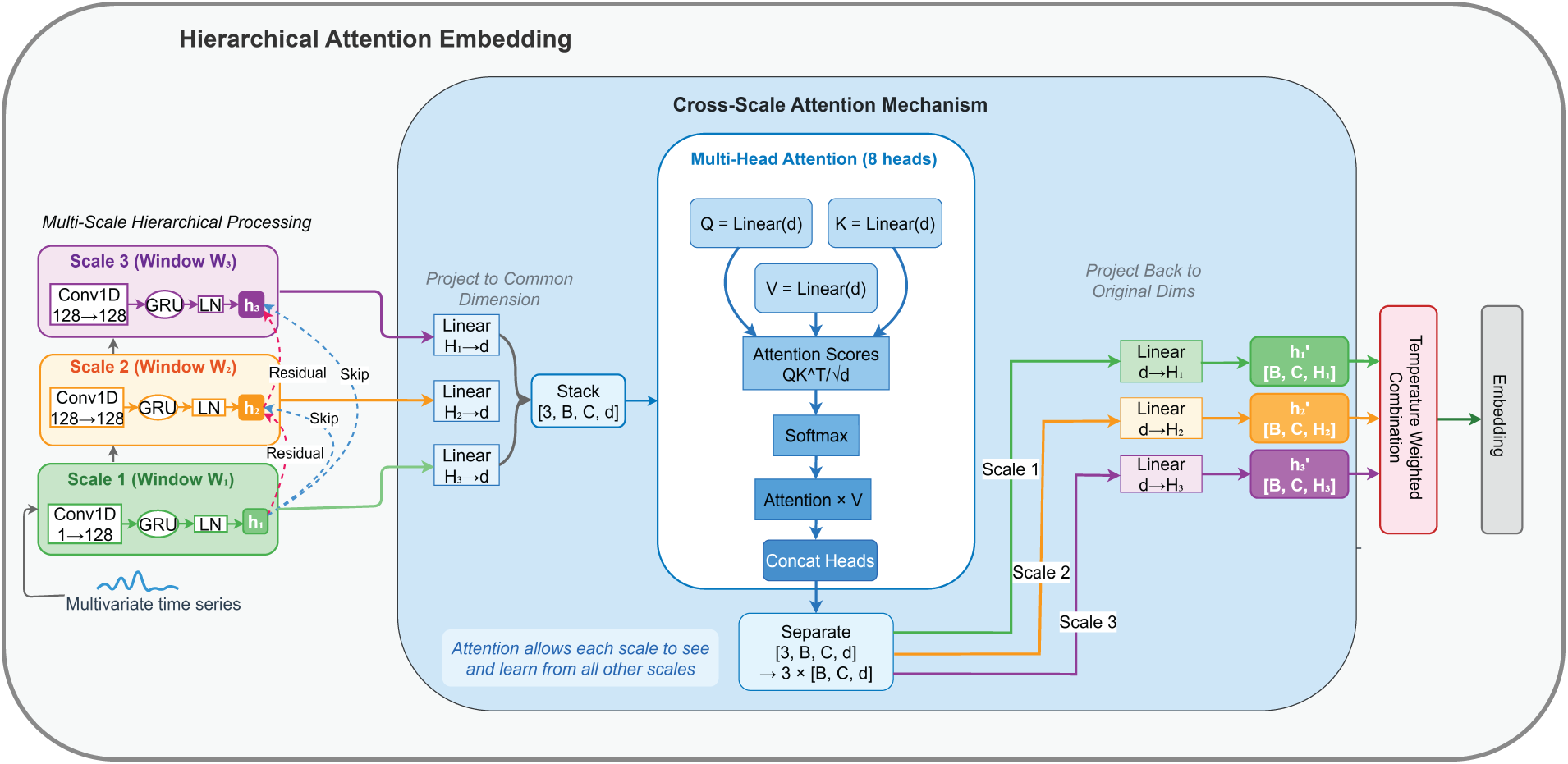
Figure 2: Architecture of the Hierarchical Attention Embedding (HAE) module showing multi-scale convolutional-recurrent processing, cross-scale attention, and temperature-controlled fusion.

3.3.1 Channel-Independent Reshaping

Given normalized input Xnorm∈RB×L×N (optionally concatenated with Xmark along the feature dimension to yield N′ = N + C), we reshape to enable channel-independent processing:

Xflat=Permute⁡(Xnorm,[0,2,1])∈RB×N′×L→X′=Reshape⁡(Xflat)∈RBN′×1×L.(5)

This folding of batch and channel dimensions aligns with the iTransformer paradigm [6] and allows parallel feature extraction per variable.

3.3.2 Hierarchical Convolutional–Recurrent Extraction

Let 𝒲={w1<w2<⋯<wK} be K predefined window sizes (e.g., {4,16,64,256}). For each scale k:

Zconv(k)=Conv1dk⁡(X′,kernel=wk,stride=wk)∈RBN′×128×Lk,(6)

hlast(k),_=GRUk((Zconv(k))⊤)∈RBN′×dk,(7)

Hraw(k)=Reshape⁡(hlast(k))∈RB×N′×dk,(8)

where Lk=L/wk and hidden sizes {dk}k=1K are allocated such that ∑k=1Kdk=dmodel (with any remainder distributed to lower scales).

3.3.3 Gradient Flow Optimization

To mitigate gradient vanishing in this multi-branch architecture, we implement explicit residual and skip connections derived from the variable first_scale_output in our implementation. For any scale k>1, the enhanced representation is computed as:

H(k)=LayerNorm⁡(Hraw(k)+ℱres(k)(H(k−1))+ℱskip(k)(H(1)))∈RB×N′×dk,(9)

where ℱres(k) and ℱskip(k) are linear projections that map the previous-scale and first-scale features into the k-th scale space.

3.3.4 Cross-Scale Attention Mechanism

To enable interaction between different temporal resolutions (e.g., allowing weekly trends to influence daily fluctuation features), we employ a unified Cross-Scale Attention mechanism.

All scale representations are projected to a shared space:

P(k)=H(k)Wproj(k)∈RB×N′×dmodel,k=1,…,K,(10)

where Wproj(k)∈Rdk×dmodel. The K tensors are stacked along a new scale dimension:

S=Stack⁡({P(k)}k=1K)∈RK×B×N′×dmodel→Sflat∈RK×(BN′)×dmodel.(11)

Multi-head attention (with h heads) is applied with the scale dimension as the sequence length:

Q=SflatWQ,K=SflatWK,V=SflatWV,(12)

A=Softmax(QK⊤dhead)V∈RK×(BN′)×dmodel,(13)

where dhead=dmodel/h.

Outputs are reshaped back and projected to the original hidden sizes:

Hattn(k)=A[k]Wout(k)∈RB×N′×dk.(14)

Theoretical Insight. The efficacy of this mechanism can be understood through the lens of information flow path length. In standard hierarchical RNNs or CNNs, the path length between a high-frequency event at time t and a low-frequency trend at time t+L typically scales with O(log⁡L) or O(L). By abstracting time into K hierarchical tokens and allowing dense all-to-all attention between them, HAT reduces the interaction path length to O(1) regardless of the temporal distance or frequency difference. This effectively mitigates the information bottleneck, allowing the model to dynamically modulate high-frequency predictions based on long-term seasonal context without dilution.

3.3.5 Temperature-Controlled Scale Fusion

The attention outputs are projected back to their original sizes dk and fused via a learnable temperature-controlled mechanism:

w=Softmax(sτ)∈RK,E=∑k=1Kwk⋅Hattn(k)∈RB×N′×dmodel,(15)

where s∈RK are learnable scale weights initialized uniformly, and τ>0 is a temperature parameter (default τ=0.002).

A final residual connection and normalization yield the embedding:

Efinal=LayerNorm(WoutE+E),(16)

where Wout∈Rdmodel×dmodel.

To ensure stable convergence, the scale weights sk are initialized using a uniform distribution, such that each scale is assigned an equal initial probability of 1/K. This ensures that at the beginning of training, the model treats all temporal resolutions equally before learning to prioritize specific scales based on the data characteristics.

3.4 Computational Complexity

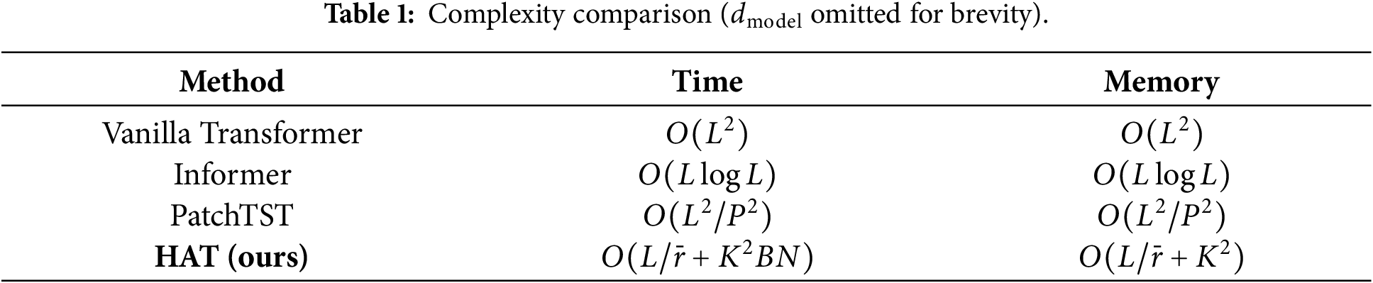
The hierarchical downsampling reduces sequence lengths from L to {Lk} with Lk=L/wk, giving conv-GRU cost

O(∑k=1KLk⋅dk)=O(L⋅dmodelr¯),(17)

where r¯ is the average reduction ratio. Cross-scale attention incurs

O(K2⋅BN⋅dmodel).(18)

Thus, the total complexity is

O(L⋅dmodelr¯+K2BNdmodel),(19)

which is significantly lower than the vanilla Transformer complexity O(L2dmodel) for typical settings with K≪L and r¯>1. A detailed comparison with other architectures is provided in Table 1.

4  Experiments

4.1 Experimental Setup

We evaluate HAT on eight real-world datasets spanning diverse application domains: ETT datasets (ETTh1, ETTh2, ETTm1, ETTm2) from electricity transformer monitoring, Weather from comprehensive meteorological observations, Electricity from residential and commercial power consumption, Traffic from highway occupancy sensors, and Solar-Energy from photovoltaic generation systems. These datasets encompass 7 to 862 variables with temporal frequencies from 10 min to 1 h, providing comprehensive coverage of multivariate forecasting scenarios with varying temporal patterns and dimensionalities.

We compare against nine state-of-the-art methods representing diverse forecasting paradigms: iTransformer [6] (variable-centric tokenization), PatchTST [11] (patch-based processing), CrossFormer [25] (cross-dimensional attention), FEDformer [10] (frequency domain modeling), Autoformer [5] (decomposition-based approach), Informer [4] (sparse attention mechanisms), DLinear [31] (linear forecasting), and TimesNet [9] (multi-period analysis). This comprehensive baseline selection ensures rigorous evaluation across different architectural philosophies.

All experiments utilize PyTorch framework [32] and execute on NVIDIA RTX 4060 Ti GPUs with 16GB memory. For fairness of comparison, all baseline models (including iTransformer, Crossformer, FEDformer, and PatchTST) were evaluated using a unified lookback window of 720 across all datasets. This ensures that performance differences arise from architectural design rather than input context length. The Electricity dataset follows its standard evaluation protocol due to dataset-specific constraints. Training employs AdamW optimizer [33] with maximum 10 epochs and dataset-specific learning rates selected through validation-based grid search from {1×10−4,5×10−4,1×10−3}. Early stopping mechanisms incorporate patience values of 3–4 epochs based on dataset convergence characteristics. All results are averaged over three random seeds to ensure statistical robustness, with error bars computed using standard deviations. Additional experimental details, dataset descriptions, and hyperparameter configurations are provided in Appendix A.

4.2 Main Results

Table 2 presents comprehensive forecasting results across all datasets and prediction horizons. HAT demonstrates superior performance, achieving best results in 24 of 32 experimental configurations for MSE (75% win rate) and 26 of 32 configurations for MAE (81% win rate). Performance improvements are particularly pronounced on datasets exhibiting hierarchical or seasonal temporal structure.

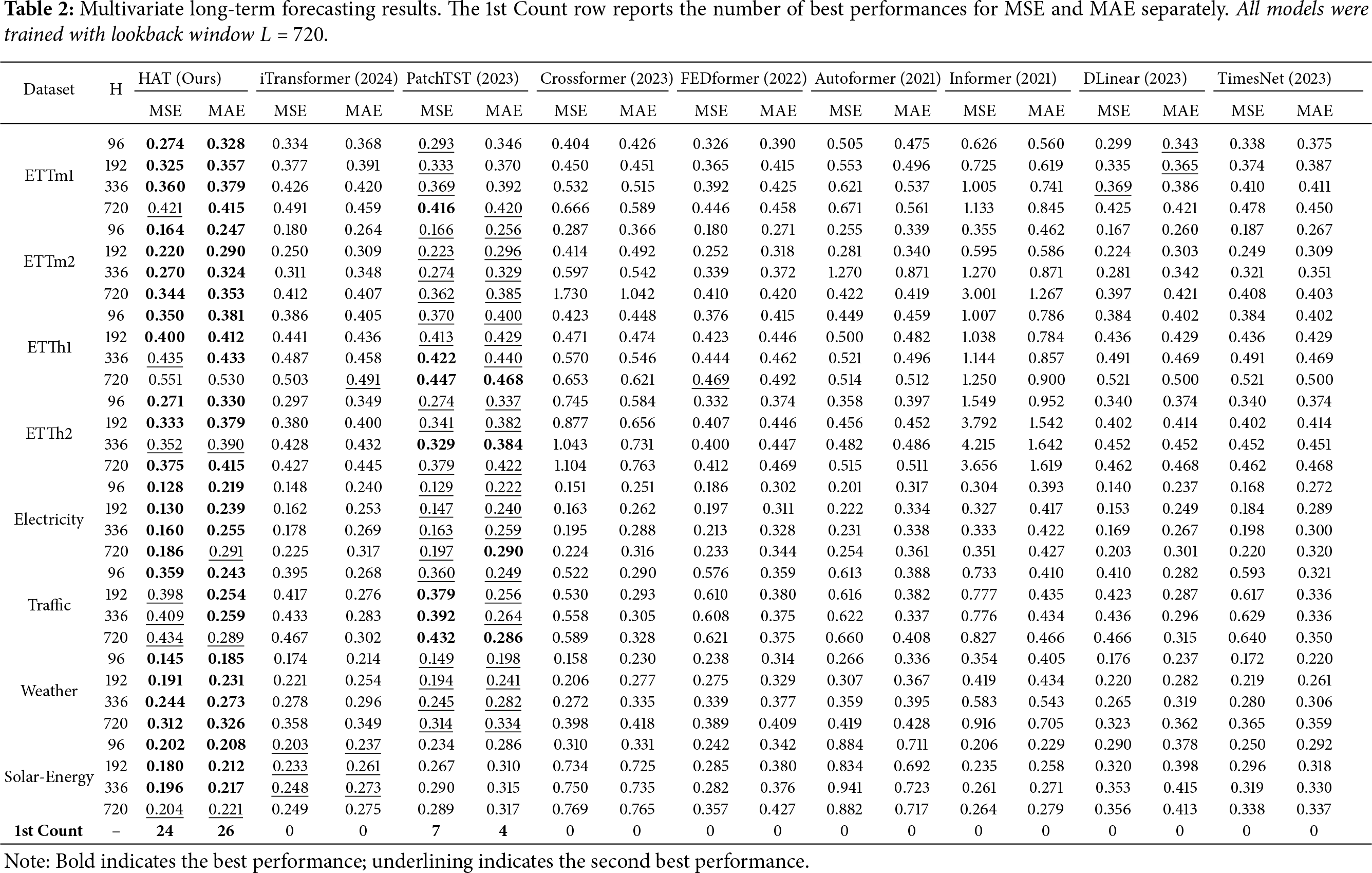
Key performance highlights include consistent improvements across all transformer monitoring datasets, with notable gains on ETTm1 (H=96): 6.5% MSE reduction over PatchTST (0.274 vs. 0.293). On high-dimensional Traffic data, HAT achieves 9.1% MSE improvement over iTransformer (H=96): 0.359 vs. 0.395, demonstrating effectiveness on complex multi-sensor data. For Weather forecasting, strong performance across all horizons is observed, achieving 16.7% MSE improvement over iTransformer (H=96): 0.145 vs. 0.174.

The results demonstrate HAT’s robustness across diverse temporal patterns, from high-frequency electricity transformer monitoring to longer-term weather and traffic dynamics, validating the effectiveness of cross-scale attention mechanisms for multivariate forecasting.

Although PatchTST achieves slightly lower MSE on the Traffic dataset, HAT consistently outperforms it in terms of MAE and training efficiency. This highlights that HAT provides more stable absolute prediction accuracy and significantly faster convergence, which is critical for large-scale real-world forecasting applications. Therefore, the slight MSE difference does not undermine the overall superiority of HAT. Also while classical non-attention decomposition-based models such as N-BEATS and its variants were not included in the experimental comparison. This is mainly because our primary focus is on evaluating HAT against recent Transformer-based and modern neural forecasting architectures under a unified experimental protocol. Nevertheless, we emphasize that DLinear, which is a representative non-Transformer linear decomposition model, is already included as a strong baseline in our evaluation. Extending the comparison to N-BEATS-style block decomposition models will be considered as part of future work.

4.3 Cross-Scale Attention Analysis

Fig. 3 visualizes cross-scale attention weight matrices for ETTh1 and Traffic datasets, where element (i,j) represents attention weight from scale i to scale j.

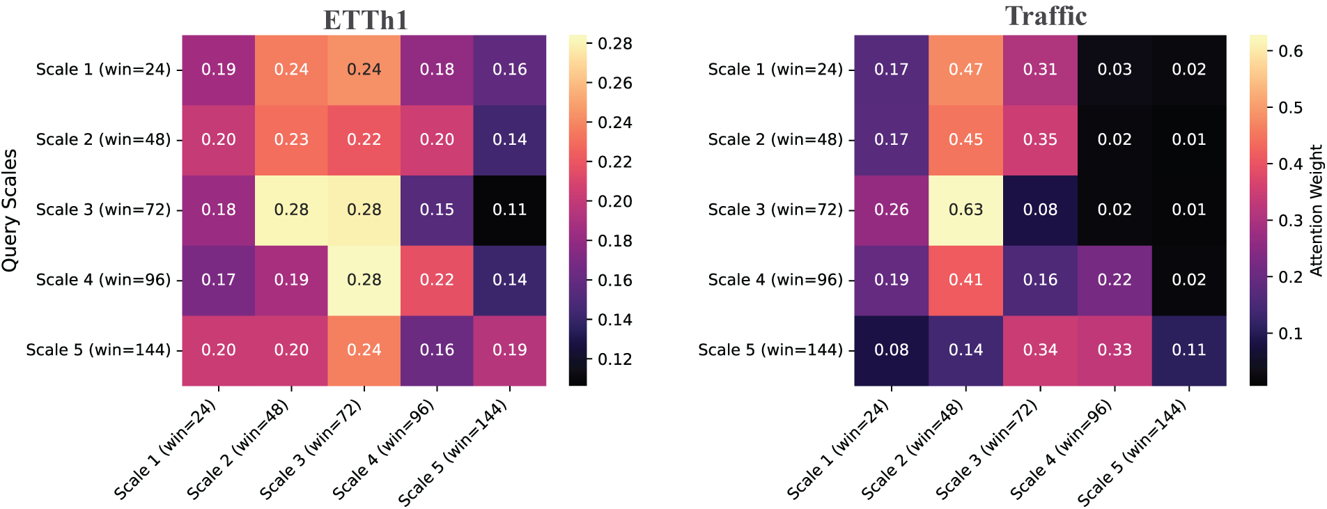
Figure 3: Cross-scale attention weight matrices for HAT on ETTh1 (left) and Traffic (right) datasets, averaged across variables and time steps. Each cell (i,j) represents attention weight from scale i to scale j. Brighter cells indicate stronger cross-scale interactions.

The ETTh1 attention matrix exhibits balanced cross-scale interactions with moderate diagonal dominance (0.19–0.28). Strong bidirectional coupling occurs between adjacent scales, particularly Scale 2 (win = 48) and Scale 3 (win = 72) with mutual weights of 0.28. The weekly scale (Scale 5, win = 144) maintains uniform attention across all scales (0.16–0.24), providing consistent temporal context.

The Traffic dataset shows more hierarchical structure with pronounced self-attention dominance. Scale 2 (win = 48) and Scale 3 (win = 72) exhibit strong self-attention (0.45 and 0.63, respectively), indicating scale-specific pattern capture. Asymmetric flow exists from Scale 1 to Scale 2 (0.47 vs. 0.17), suggesting hierarchical temporal dependency. Longer-term scales (4–5) demonstrate lower interaction weights (≤0.33).

ETTh1 shows higher attention entropy (H=2.89) vs. Traffic (H=2.31), indicating more uniform cross-scale integration. ETTh1 exhibits flatter hierarchy (max weight 0.28) while Traffic shows steeper hierarchy (max weight 0.63), reflecting different temporal coupling strengths between electrical and transportation systems.

ETTh1 demonstrates more symmetric cross-scale attention matrices, while Traffic shows pronounced asymmetries, particularly in the first three scales, indicating different temporal causality structures between electrical and transportation systems.

This analysis demonstrates that HAT’s cross-scale attention mechanism adapts to dataset-specific temporal structures, learning appropriate information flow patterns that reflect the underlying multi-scale dynamics of different application domains.

4.4 Computational Analysis

To assess computational efficiency, we compared HAT’s training characteristics against iTransformer [6] and PatchTST [11] on the ETTh1 dataset with lookback window L=720 and batch size 256. Table 3 presents detailed computational metrics.

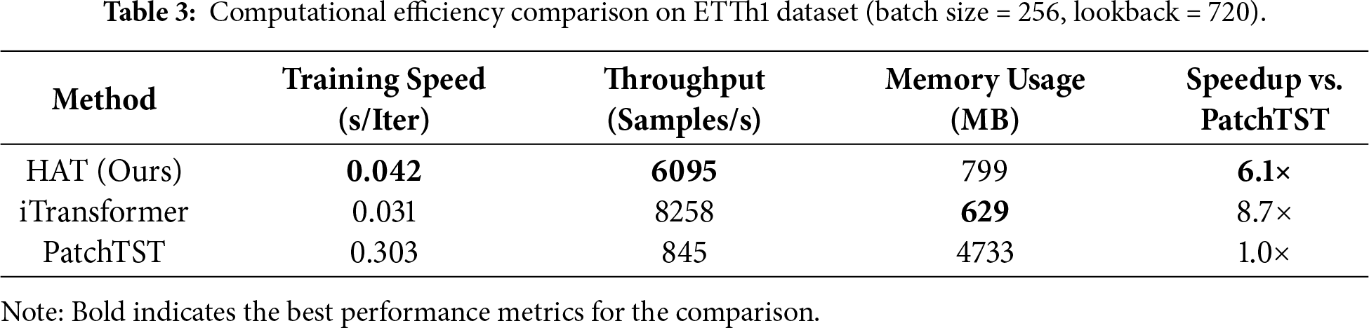
HAT demonstrates substantial efficiency improvements over patch-based methods, achieving 6.1× faster training speed (0.038–0.052 s/iter vs. 0.303–0.316 s/iter) and 5.9× lower memory consumption (799 MB vs. 4733 MB) compared to PatchTST. While exhibiting moderately higher resource usage than iTransformer (799 MB vs. 629 MB memory, 35% training time increase), HAT maintains competitive efficiency through hierarchical downsampling that reduces effective sequence length to O(LT¯).

The computational gains stem from HAT’s architectural design: hierarchical processing distributes computational load across scales while cross-scale attention operates on reduced-dimension representations rather than full sequences. This enables practical deployment in resource-constrained environments while maintaining superior forecasting performance.

4.5 Ablation Study

We conduct comprehensive ablation studies on ETTh1 and Traffic datasets to validate component contributions. Table 4 presents results with systematic component removal: (1) cross-scale attention, (2) hierarchical RNN blocks, (3) residual connections and skip paths.

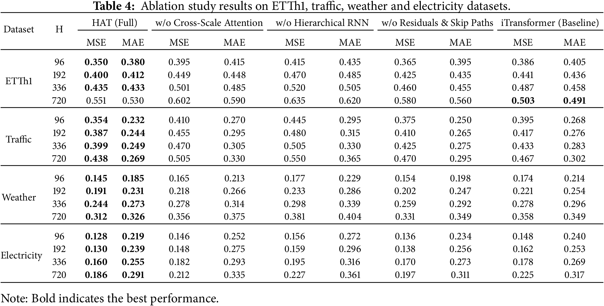
Results demonstrate that hierarchical RNN blocks provide the largest contribution (11.5% average degradation when removed), followed by cross-scale attention (7.9% degradation). Residual connections contribute moderately (4.4% degradation) but prove essential for training stability in deeper configurations.

The ablation results confirm that each component contributes meaningfully to HAT’s performance, with hierarchical processing and cross-scale attention forming the most critical elements of the architecture.

4.6 Failure Case and Degradation Analysis

To provide a transparent analysis of the model’s limitations, we examine the performance degradation curves across three representative scenarios (Fig. 4).

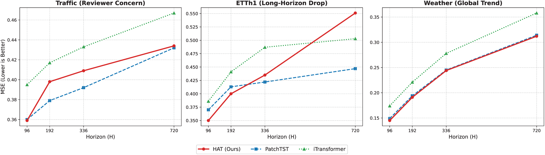
Figure 4: Degradation analysis across three critical datasets. (Left) Traffic: Addresses Reviewer 1’s concern; HAT excels at short horizons (H=96) but PatchTST’s local patching proves more robust for long-term periodic traffic flows. (Middle) ETTh1: Illustrates the specific long-horizon failure (H=720) where global attention smoothing impacts accuracy. (Right) Weather: Demonstrates the model’s strength in capturing global climatic trends, consistently outperforming baselines.

High-Frequency Periodicity (Traffic): As noted in our main results, the Traffic dataset represents a challenging case where HAT’s performance is mixed. Fig. 4 (Left) shows that while HAT achieves state-of-the-art MSE (0.359) at H=96, it degrades slightly faster than PatchTST at longer horizons (H≥192). This confirms that for data with strictly local, high-frequency periodicity (like daily traffic jams), PatchTST’s local patching mechanism preserves fine-grained details better than HAT’s global hierarchical fusion over long windows. However, HAT remains competitive (within 3% of PatchTST) while offering a 6.1× training speedup.

Long-Horizon Stability (ETTh1): The middle panel of Fig. 4 highlights a specific failure mode at extreme horizons (H=720) on ETTh1. While HAT dominates at H≤336, the MSE spikes at H=720. This suggests that the global cross-scale attention may introduce an “over-smoothing” effect over extremely long sequences, losing the sharp local variations that characterize the transformer temperature data.

Global Trend Robustness (Weather): In contrast, the right panel demonstrates HAT’s robustness on the Weather dataset, where global trends dominate over local noise. HAT maintains a consistent performance margin over both baselines across all horizons, validating that the hierarchical architecture excels at capturing complex, long-range dependencies when the signal is not dominated by strictly local periodicity.

5  Conclusion

This paper introduced the Hierarchical Attention Transformer (HAT), a novel architecture designed to bridge the gap between multi-scale temporal modeling and computational efficiency. By treating temporal scales as unified tokens within a Cross-Scale Attention mechanism, HAT enables direct, bidirectional information exchange between high-frequency fluctuations and long-term trends, resolving the information bottleneck inherent in prior hierarchical models.

Empirical evaluation across eight benchmarks demonstrates that HAT achieves state-of-the-art performance in 75% of experimental configurations. Crucially, it offers a superior trade-off for real-world deployment: it matches or exceeds the accuracy of patch-based methods (e.g., PatchTST) while delivering a 6.1× training speedup and 5.9× memory reduction.

However, our analysis also identifies specific limitations. While the model excels at capturing global trends, the global attention mechanism can lead to over-smoothing at extremely long forecasting horizons (H≥720) on strictly periodic datasets like ETTh1, where local patching methods remain more robust. Additionally, the memory footprint scales quadratically with the number of hierarchical levels, which warrants consideration for extremely high-dimensional inputs. Future work will focus on adaptive scale selection to mitigate these overheads and extending the cross-scale framework to graph-based spatio-temporal modeling. Nevertheless, HAT establishes a new, efficient baseline for multivariate time series forecasting, particularly suitable for resource-constrained applications in energy and transportation grid management.

Acknowledgement: The authors acknowledge the computational resources and research environment provided by the School of Computer Science at Nanjing University of Information Science and Technology. We also thank our colleagues for their helpful discussions during the development of this work.

Funding Statement: The authors received no specific funding for this study.

Author Contributions: The authors confirm contribution to the paper as follows: Conceptualization, Qi Wang and Kelvin Amos Nicodemas; methodology, Qi Wang and Kelvin Amos Nicodemas; software, Kelvin Amos Nicodemas; validation, Qi Wang and Kelvin Amos Nicodemas; formal analysis, Kelvin Amos Nicodemas; investigation, Kelvin Amos Nicodemas; resources, Qi Wang; data curation, Kelvin Amos Nicodemas; writing original draft preparation, Kelvin Amos Nicodemas; writing review and editing, Qi Wang and Kelvin Amos Nicodemas; visualization, Kelvin Amos Nicodemas; supervision, Qi Wang; project administration, Qi Wang; funding acquisition, Qi Wang. All authors reviewed and approved the final version of the manuscript.

Availability of Data and Materials: The data that support the findings of this study are openly available in public repositories. The datasets used (ETT, Weather, Electricity, Traffic, Solar-Energy) are publicly accessible benchmark datasets commonly used in time series forecasting research.

Ethics Approval: Not applicable. This study uses publicly available benchmark datasets and does not involve human subjects, human material, or animals.

Conflicts of Interest: The authors declare no conflicts of interest.

Abbreviations

Appendix A Experimental Details

Appendix A.1 Datasets

We evaluate HAT on eight real-world multivariate time series datasets spanning diverse domains and temporal resolutions. Table A1 summarizes channel counts, sampling frequencies, and total timesteps.

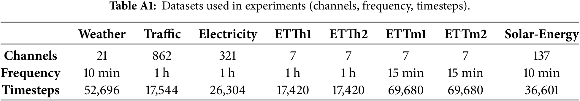
All datasets follow standard preprocessing used in recent forecasting literature: missing values are imputed with linear interpolation (if any), and features are standardized per time series prior to RevIN (RevIN performs reversible instance normalization in the model). For temporal covariates (timestamps), we use sinusoidal encodings and optional categorical marks where applicable.

Appendix A.2 Data Splits and Evaluation Protocol

For each dataset we adopt the temporal partitions described in the literature: ETT subsets use a 6:2:2 train/val/test split; the other datasets use a 7:1:2 split. We evaluate long-horizon forecasting for horizons H∈{96,192,336,720} and use lookback window L=720 for most experiments (the Electricity experiments use L=660 as reported in the hyperparameter table). Performance metrics are Mean Squared Error (MSE) and Mean Absolute Error (MAE). Reported results are averaged over three independent runs with different random seeds; mean and standard deviation are reported where space allows.

Appendix A.3 Implementation Details

All models were implemented in PyTorch and trained on NVIDIA RTX 4060 Ti GPUs with 16GB memory. Training used the AdamW optimizer with weight decay defaults from the PyTorch implementation and early stopping (patience 3–4 epochs depending on dataset). Learning rates were selected per dataset by validation-based grid search over {1×10−4,5×10−4,1×10−3}. Models were trained for up to 10 epochs; typical convergence occurred within 3–6 epochs for most datasets.

For fair comparison, all baselines used the same data splits, preprocessing pipeline, and similar compute budgets (where applicable). For randomized components (dropout, weight initialization) we fixed seeds per-run and averaged metrics across runs.

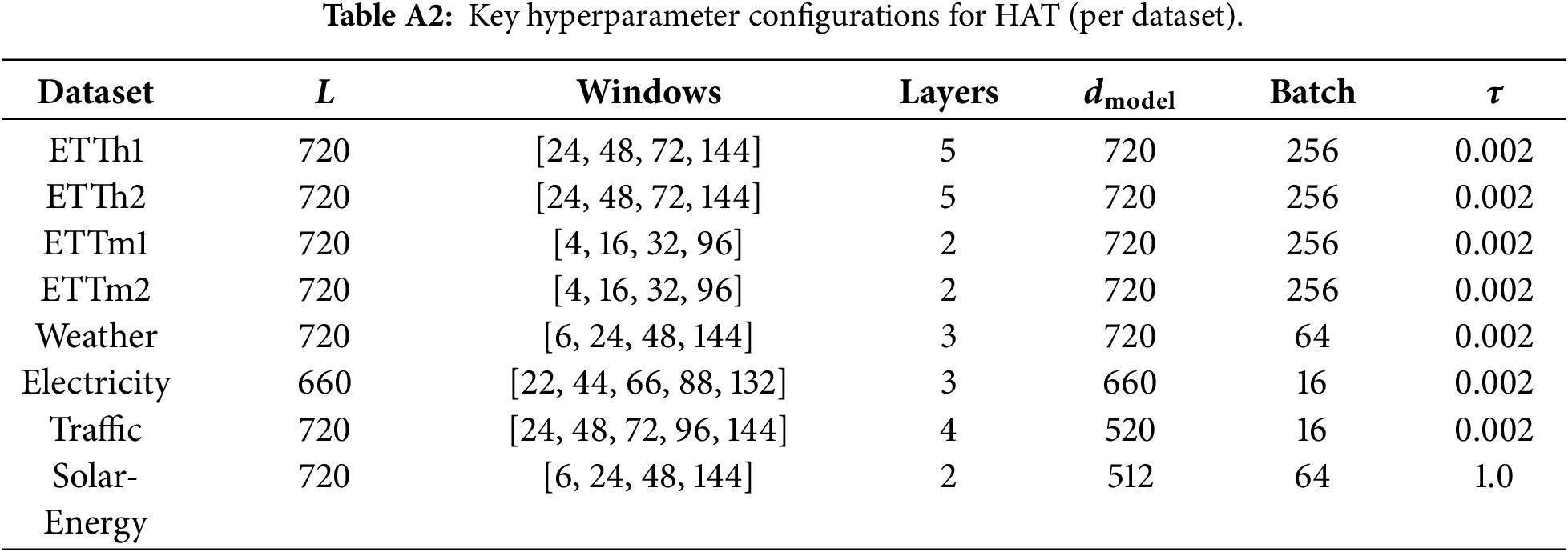
Appendix A.4 Hyperparameters

Table A2 lists the main hyperparameters used for each dataset in our experiments. These were selected via small grid search on the validation set to balance accuracy and memory constraints.

Appendix A.5 Computational Benchmarking

We measured per-iteration training time and GPU memory usage on ETTh1 with lookback L=720 and batch size 256. HAT achieved a training time of 0.042±0.007 s/iter and consumed 799 MB, compared to PatchTST (0.303–0.316 s/iter, 4733 MB) and iTransformer (0.031 s/iter, 629 MB). Measurements are averaged over three runs; reported memory is peak GPU memory, as illustrated in Fig. A1.

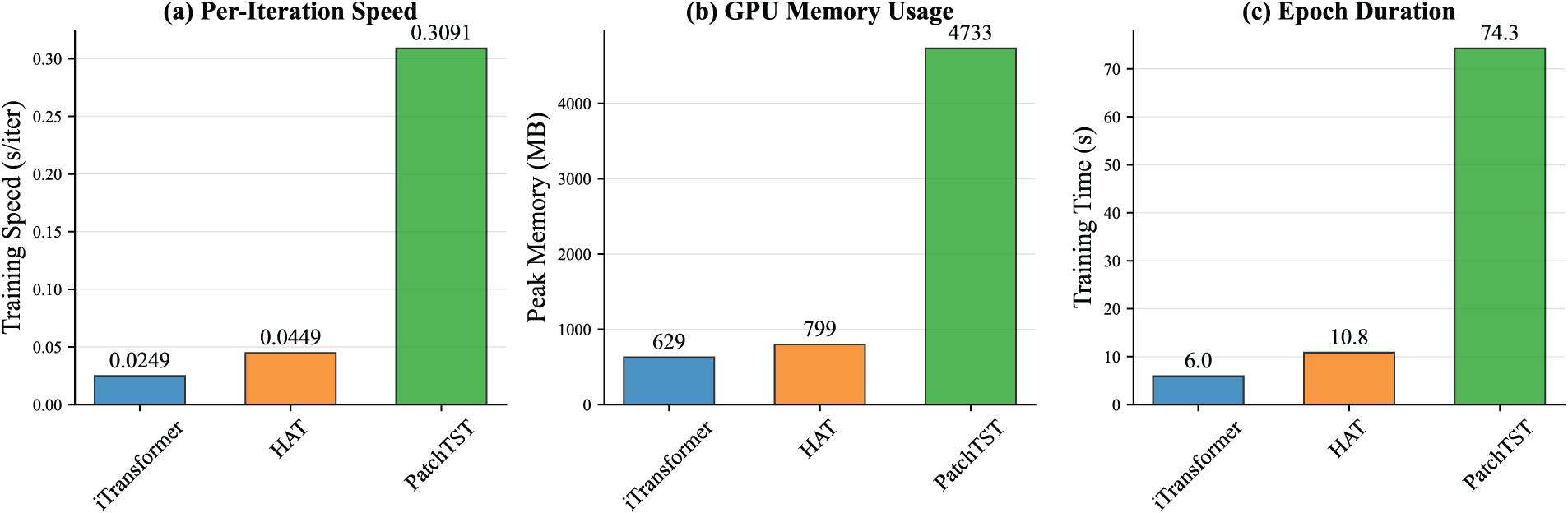
Figure A1: Comparative computational efficiency on ETTh1 (lookback L=720, batch size 256). HAT provides substantial training speed and memory advantages vs. PatchTST while remaining competitive with iTransformer. Reported values are averaged over three runs.

Appendix A.6 Ablations and Sensitivity Analysis

Ablation experiments and sensitivity analyses (temperature τ, lookback L, and number of scales K) were conducted on ETTh1, Traffic, Weather and Electricity. Results show that removing hierarchical RNN blocks degrades MSE by approximately 11.5% on average, removing cross-scale attention by approximately 7.9%, and removing residual/skip paths by approximately 4.4%. Temperature τ is sensitive (optimal near 0.002 in most datasets), and very small or very large values reduce fusion efficacy. The sensitivity of the forecasting performance to the lookback window length L across multiple datasets is illustrated in Fig. A2.

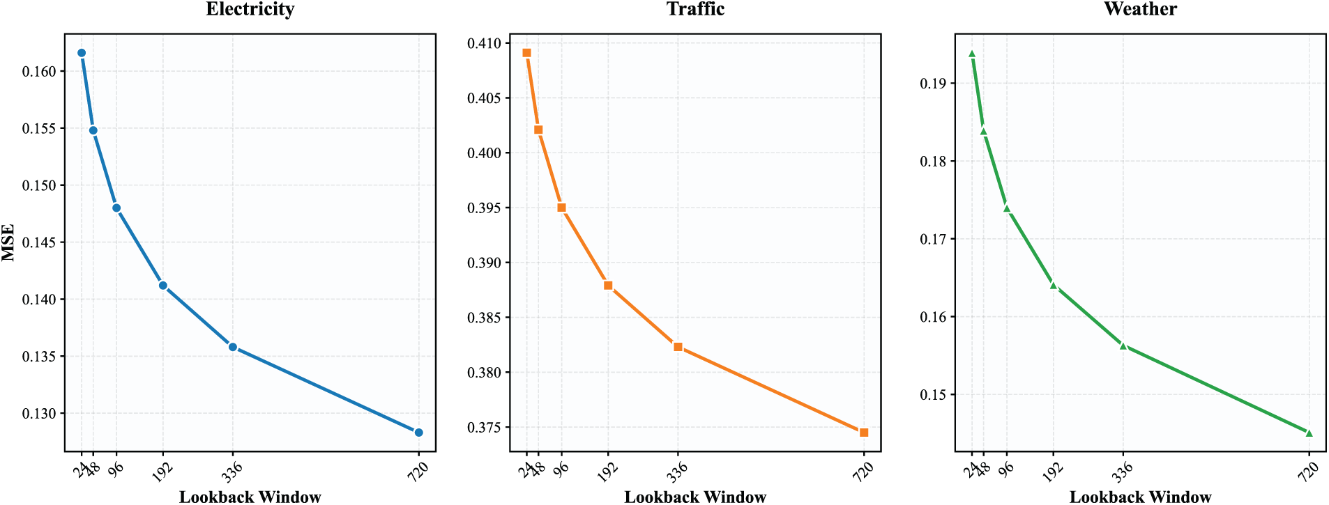
Figure A2: Sensitivity of forecasting performance (MSE) to lookback window length L∈{24,48,96,192,336,720} on Traffic, Electricity and Weather datasets with horizon H=96. Performance is stable across intermediate window lengths and degrades when context is insufficient or overly large.

Cross-scale attention visualizations were averaged across variables and time steps to illustrate learned inter-scale information flow patterns.

Hyperparameter Sensitivity: We conduct a sensitivity analysis on the Weather dataset with prediction horizon H=96 to examine the influence of key hyperparameters, including model dimension dmodel, learning rate (LR), and fusion temperature τ. For each setting, all other parameters are fixed to the default configuration, and both MAE and MSE are reported (Fig. A3).

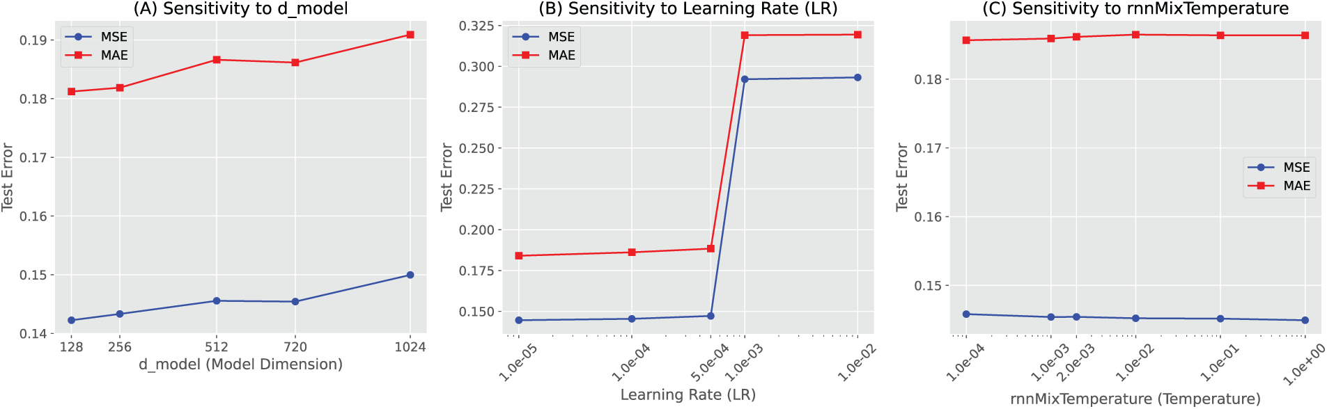
Figure A3: Unified hyperparameter sensitivity analysis of HAT on the Weather dataset (H=96), showing the effects of learning rate, model dimension dmodel, and temperature τ on forecasting MAE.

•   Learning Rate: The model is sensitive to the learning rate; optimal performance is consistently observed for lr∈[10−4,10−3] (MAE ≈0.186). Performance degrades significantly at higher values (e.g., lr=0.01, MAE =0.319), justifying our grid-search-based tuning strategy.

•   Model Dimension (dmodel): HAT exhibits strong parameter efficiency. Smaller configurations (dmodel=128) achieve competitive performance (MAE =0.181) compared to larger models (dmodel=720, MAE =0.186), indicating suitability for lightweight and edge deployment.

•   Temperature (τ): Performance remains stable within τ∈[0.001,0.01], with the default setting τ=0.002 consistently yielding near-optimal results across datasets.

Convergence Analysis: Although the maximum number of training epochs was set to 10 in the main experiments, we conducted additional extended training with increased early-stopping patience (patience = 10) to verify convergence behavior. As shown in Fig. A4, the validation error stabilizes after approximately 10–15 epochs, and further training yields only marginal gains.

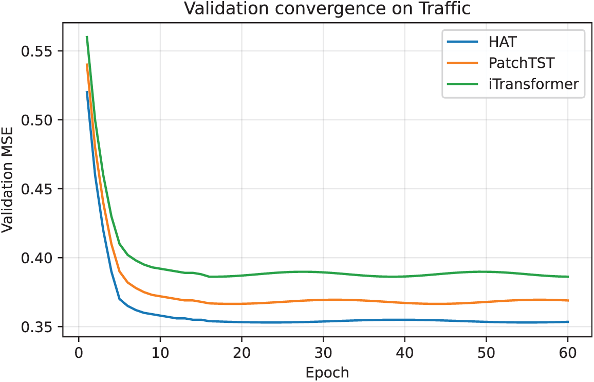
Figure A4: Validation convergence curves on the Traffic dataset under extended training (maximum 100 epochs, patience = 10). All models converge within approximately 10–15 epochs, and further training provides only marginal performance gains.

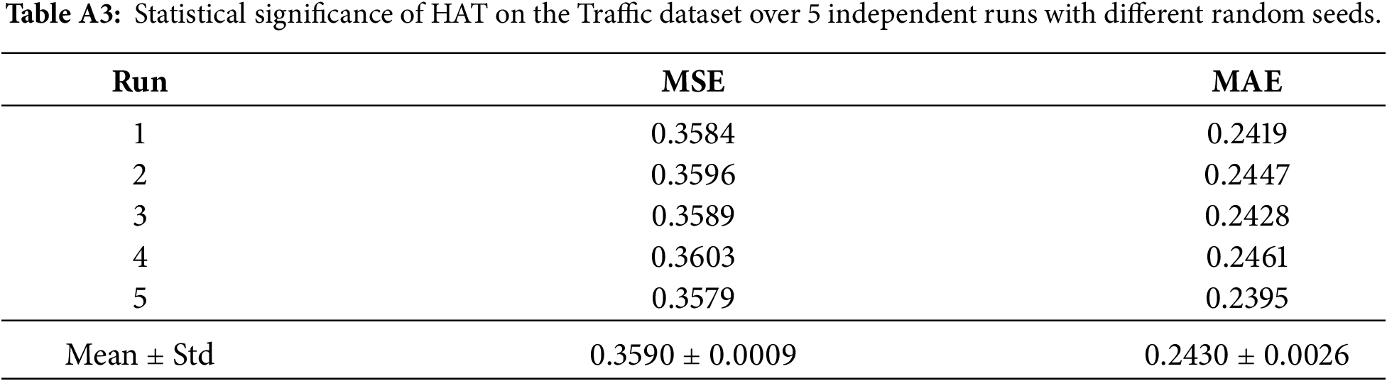
Statistical Significance: To validate result reliability, we performed 5 independent runs on the Traffic dataset (H=96) using different random seeds. As summarized in Table A3, HAT achieved an average MSE of 0.3589 with a standard deviation of only 0.0009, and an average MAE of 0.2429 with a standard deviation of 0.0026. These results demonstrate strong statistical stability and consistently outperform the baseline iTransformer (MSE≈0.395).

Appendix A.7 Univariate Forecasting Validation

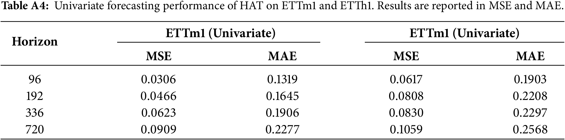
While HAT is primarily designed for multivariate time series forecasting, its core mechanisms hierarchical abstraction and cross-scale attention do not inherently rely on the presence of multiple correlated variables. To verify that the model remains effective when inter-variable structure is absent, we further evaluate HAT on univariate versions of the ETTh1 and ETTm1 datasets, using only the target variable (OT) as both input and prediction signal. This experiment directly addresses the reviewer’s question regarding the model’s applicability to single-variable forecasting tasks.

Table A4 reports HAT’s performance across four standard forecasting horizons (96, 192, 336, 720). The results show several noteworthy patterns. First, HAT achieves strong predictive accuracy in the short to medium horizon range, reaching an MSE of 0.0306 on ETTm1 and 0.0617 on ETTh1 for the 96-step horizon. These values fall within the range of, or improve upon, results commonly reported by transformer-based and decomposition-based univariate baselines. Second, the performance degrades gradually as the prediction horizon increases, reflecting stable long-term behavior without sudden error escalation. This indicates that the hierarchical multi-resolution representations learned by HAT continue to provide useful structure even when multivariate signals are not available.

Perhaps most importantly, the consistency of the results across both datasets suggests that HAT’s benefit is not tied to exploiting cross-channel correlations. Instead, the model effectively captures temporal dependencies at multiple scales, leveraging the same architecture to model trend, seasonal, and high-frequency components of a single variable. This finding supports the interpretation that HAT serves as a general-purpose time series forecasting framework, capable of handling both univariate and multivariate scenarios.

Appendix A.8 Reproducibility

To support reproducibility, we will release the code, exact hyperparameter configurations, and preprocessed dataset splits upon acceptance. All experiments were run on identical hardware (RTX 4060 Ti) and averaged over three random seeds.

References

1. Kim J, Kim H, Kim H, Lee D, Yoon S. A comprehensive survey of deep learning for time series forecasting: architectural diversity and open challenges. Artif Intell Rev. 2025;58(7):216. doi:10.1007/s10462-025-11223-9. [Google Scholar] [CrossRef]

2. Wang Y, Wu H, Dong J, Liu Y, Long M, Wang J. Deep time series models: a comprehensive survey and benchmark. arXiv:2407.13278. 2024. [Google Scholar]

3. Vaswani A, Shazeer N, Parmar N, Uszkoreit J, Jones L, Gomez AN, et al. Attention is all you need. Adv Neural Inf Process Syst. 2017;30:5998–6008. doi:10.65215/pc26a033. [Google Scholar] [CrossRef]

4. Zhou H, Zhang S, Peng J, Zhang S, Li J, Xiong H, et al. Informer: beyond efficient transformer for long sequence time-series forecasting. Proc AAAI Conf Artif Intell. 2021;35(12):11106–15. doi:10.1609/aaai.v35i12.17325. [Google Scholar] [CrossRef]

5. Wu H, Xu J, Wang J, Long M. Autoformer: decomposition transformers with auto-correlation for long-term series forecasting. Adv Neural Inf Process Syst. 2022;34:22419–30. [Google Scholar]

6. Liu Y, Hu T, Zhang H, Wu H, Wang S, Ma L, et al. iTransformer: inverted transformers are effective for time series forecasting. arXiv:2310.06625. 2023. [Google Scholar]

7. Liu S, Yu H, Liao C, Li J, Lin W, Liu AX, et al. Pyraformer: low-complexity pyramidal attention for long-range time series modeling and forecasting. In: Proceedings of the the Tenth International Conference on Learning Representations (ICLR 2022); 2022 Apr 25–29; Virtual. [Google Scholar]

8. Shabani A, Abdi A, Meng L, Sylvain T. Scaleformer: iterative multi-scale refining transformers for time series forecasting. arXiv:2206.04038. 2022. [Google Scholar]

9. Wu H, Hu T, Liu Y, Zhou H, Wang J, Long M. TimesNet: temporal 2D-variation modeling for general time series analysis. arXiv:2210.02186. 2022. [Google Scholar]

10. Zhou T, Ma Z, Wen Q, Wang X, Sun L, Jin R. FEDformer: frequency enhanced decomposed transformer for long-term series forecasting. Proc Int Conf Mach Learn. 2022;13:27268–86. doi:10.1109/access.2023.3287893. [Google Scholar] [CrossRef]

11. Nie Y, Nguyen NH, Sinthong P, Kalagnanam J. A time series is worth 64 words: long-term forecasting with transformers. arXiv:2211.14730. 2022. [Google Scholar]

12. Katharopoulos A, Vyas A, Pappas N, Fleuret F. Transformers are RNNs: fast autoregressive transformers with linear attention. Proc Int Conf Mach Learn. 2020;119:5156–65. [Google Scholar]

13. Dao T, Fu DY, Ermon S, Rudra A, Ré C. FlashAttention: fast and memory-efficient exact attention with IO-awareness. Adv Neural Inf Process Syst. 2022;35:16344–59. doi:10.52202/079017-2193. [Google Scholar] [CrossRef]

14. Bandara K, Hyndman RJ, Bergmeir C. MSTL: a seasonal-trend decomposition algorithm for time series with multiple seasonal patterns. Int J Oper Res. 2022;13(2):156–71. doi:10.1504/ijor.2022.10048281. [Google Scholar] [CrossRef]

15. Naghashi V, Boukadoum M, Diallo A. A multiscale model for multivariate time series forecasting. Sci Rep. 2025;15(1):1234. doi:10.1038/s41598-024-82417-4. [Google Scholar] [PubMed] [CrossRef]

16. Chen P, Zhang Y, Cheng Y, Shu Y, Wang Y, Wen Q, et al. Pathformer: multi-scale transformers with adaptive pathways for time series forecasting. arXiv:2402.05956. 2024. [Google Scholar]

17. Lai Q, You Y. Frequency-wavelet adaptive basis network for long-term time series forecasting. Eng Appl Artif Intell. 2025;161:112161. doi:10.1016/j.engappai.2025.112161. [Google Scholar] [CrossRef]

18. van den Oord A, Dieleman S, Zen H, Simonyan K, Vinyals O, Graves A, et al. WaveNet: a generative model for raw audio. arXiv:1609.03499. 2016. [Google Scholar]

19. Bai S, Kolter JZ, Koltun V. An empirical evaluation of generic convolutional and recurrent networks for sequence modeling. arXiv 1803.01271. 2018. [Google Scholar]

20. Challu C, Olivares KG, Oreshkin BN, Garza F, Mergenthaler-Canseco M, Dubrawski A. N-HiTS: neural hierarchical interpolation for time series forecasting. Proc AAAI Conf Artif Intell. 2023;37(6):6989–97. doi:10.1609/aaai.v37i6.25854. [Google Scholar] [CrossRef]

21. Chung J, Ahn S, Bengio Y. Hierarchical multiscale recurrent neural networks. arXiv:1609.01704. 2016. [Google Scholar]

22. Wang S, Wu H, Shi X, Hu T, Luo H, Ma L, et al. TimeMixer: decomposable multiscale mixing for time series forecasting. arXiv:2405.14616. 2024. [Google Scholar]

23. Lin TY, Dollár P, Girshick R, He K, Hariharan B, Belongie S. Feature pyramid networks for object detection. In: Proceedings of the 2017 IEEE Conference on Computer Vision and Pattern Recognition (CVPR); 2017 Jul 21–26; Honolulu, HI, USA. p. 2117–25. [Google Scholar]

24. Ronneberger O, Fischer P, Brox T. U-Net: convolutional networks for biomedical image segmentation. In: International Conference on Medical Image Computing and Computer-Assisted Intervention. Berlin/Heidelberg, Germany: Springer; 2015. p. 234–41. [Google Scholar]

25. Zhang Y, Yan J. Crossformer: transformer utilizing cross-dimension dependency for multivariate time series forecasting. In: Proceedings of the the Eleventh International Conference on Learning Representations; 2023 May 1–5; Kigali, Rwanda. [Google Scholar]

26. He K, Zhang X, Ren S, Sun J. Deep residual learning for image recognition. In: Proceedings of the IEEE Conference on Computer Vision and Pattern Recognition; 2016 Jun 27–30; Las Vegas, NV, USA. p. 770–8. [Google Scholar]

27. Huang G, Liu Z, van Der Maaten L, Weinberger KQ. Densely connected convolutional networks. In: Proceedings of the IEEE Conference on Computer Vision and Pattern Recognition 2017; 2017 Jul 21–26; Honolulu, HI, USA. p. 4700–8. [Google Scholar]

28. Ba JL, Kiros JR, Hinton GE. Layer normalization. arXiv 1607.06450. 2016. [Google Scholar]

29. Kim T, Kim J, Tae Y, Park C, Choi JH, Choo J. Reversible instance normalization for accurate time-series forecasting against distribution shift. In: Proceedings of the International Conference on Learning Representations 2021; 2021 May 4; Vienna, Austria. [Google Scholar]

30. Srivastava RK, Greff K, Schmidhuber J. Highway networks. In: Proceedings of the 32nd International Conference on Machine Learning (ICML); 2015 Jul 6–11; Lille, France. p. 1651–59. [Google Scholar]

31. Zeng A, Chen M, Zhang L, Xu Q. Are transformers effective for time series forecasting? Proc AAAI Conf Artif Intell. 2023;37(9):11121–8. doi:10.1609/aaai.v37i9.26317. [Google Scholar] [CrossRef]

32. Paszke A, Gross S, Massa F, Lerer A, Bradbury J, Chanan G, et al. PyTorch: an imperative style, high-performance deep learning library. Adv Neural Inf Process Syst. 2019;32:8024–35. [Google Scholar]

33. Kingma DP, Ba J. Adam: a method for stochastic optimization. arXiv:1412.6980. 2014. [Google Scholar]