QPred: A Lightweight Deep Learning-Based Web Pipeline for Accessible and Scalable Streamflow Forecasting

1  Introduction

Streamflow, or river discharge, is a volumetric flow of water moving through a river channel over time and is a critical component of the hydrological cycle. Accurate streamflow forecasting is essential for flood forecasting, reservoir operations management, irrigation schedule planning, hydropower generation, and sustainable water resource management [1,2]. However, the intensity and duration of precipitation, previous rainfall conditions, temperature variations, watershed shape, deforestation, urbanization, and geological features like porosity and permeability are just a few of the many hydroclimatic and human-induced factors that influence streamflow variability [3]. Therefore, precise streamflow forecasting remains complex despite advancements in hydrological modelling [4].

Researchers have developed conceptual, physical, and data-driven models to address these issues, each possessing specific advantages and disadvantages that vary depending on the context [5]. Conceptual models are inherently simplified and are generally based on empirical formulas and are therefore rarely utilised. Physically based models, such as Soil and Water Assessment Tool (SWAT), TOPMODEL, MIKE SHE, and Hydrological Simulation Program-FORTRAN (HSPF), use physics-based formulae to simulate fundamental hydrological processes. These models necessitate substantial computational resources, specialized expertise, and accurate input data, including information on terrain, climate, soil, and land cover, thereby providing a comprehensive understanding of catchment-scale hydrological dynamics [6,7]. However, due to these processing demands and high data requirements, their usage for streamflow forecasting is still constrained [8].

Data-driven models, specifically conventional machine learning models such as random forest (RF) [9,10], support vector machine (SVM) [11] and artificial neural networks (ANN) [9,12], as well as more recent Transformer-based architectures and their variants (e.g., attention mechanisms, encoder-decoder structures) [13], have been widely used for streamflow prediction with the advancement of the artificial intelligence (AI) field. These models are capable of learning non-linear patterns, making them effective in complex hydrological modelling than traditional physics-based hydrological modelling [12]. However, conventional machine learning models frequently encounter limitations in managing temporal dependencies, which are a crucial element in hydrological modelling. Therefore, despite their simplicity and widespread adoption, conventional machine learning models are incapable of detecting both short-term and long-term dependencies, rendering them ineffective in dynamic hydrological environments [14].

Therefore, DL models, particularly recurrent neural networks (RNNs), have emerged and recently demonstrated considerable potential in modelling sequential data, with long short-term memory (LSTM) and gated recurrent unit (GRU) networks being the most prominent [15]. Hochreiter and Schmidhuber [16] introduced LSTM, an improved version of a typical RNN, to effectively capture long-term and short-term dependencies and it has been applied in many studies [17–20]. Additionally, Cho et al. [21] introduced the GRU model, a simplified variant of the LSTM by integrating short-term and long-term memory cells into a single gate, resulting in faster computational performance [22,23]. Both models generally demonstrate effective performance; however, their relative accuracy varies depending on the context, differing data processing techniques, and data input variations, with some studies reporting superior results with LSTMs, whilst others find GRUs to be more precise [22–24].

Although DL models have been increasingly adopted in hydrological modelling as alternatives to traditional physics-based approaches, their practical application within accessible, user-friendly platforms remains limited. While operational DL applications may exist in some organizations, they are rarely documented or shared in peer-reviewed literature. In contrast, traditional hydrological models, despite their complex physics-based formulas, are often embedded within user-friendly software platforms that facilitate their widespread and effective use by practitioners. Several web-based applications have been developed for various practical hydrological scenarios [25], but no or limited studies [26] have yet integrated DL-based hydrological models into such applications with documented workflows. This discrepancy is partially attributable to the interdisciplinary expertise, infrastructure requirements, and lack of accessible frameworks required for these projects, highlighting the significant need for documented, reproducible DL-powered tools in hydrological practice.

Therefore, this study aims to bridge the gap between advanced deep learning models and their practical deployment for streamflow prediction. The main contributions of this research are as follows,

•   From field data acquisition in ungauged Himalayan watersheds (Aglar and Paligaad) to operational web-based deployment, providing a reproducible framework for hydrological practitioners.

•   Systematic comparison of four deep learning architectures (vanilla LSTM, stacked LSTM, bidirectional LSTM, and GRU) for daily streamflow forecasting using standardized hydrological metrics (NSE, R2, RSR, and PBIAS).

•   Development of QPred, a lightweight, open, region-specific web application utilizing freely available cloud infrastructure (Google Colab, Flask, Google Drive, and Ngrok), eliminating the need for expensive computational resources or specialized expertise.

•   Demonstration of a reproducible pipeline that can be adapted and deployed for other watersheds and hydrological applications globally.

The remainder of this paper is organized as follows: Section 2 describes the materials and methods, including the study area characteristics, data acquisition procedures, deep learning model architectures and development, performance evaluation metrics, and web application development workflow. Section 3 presents the results and discussions, including model performance evaluation through hydrographs, statistical metrics, and scatterplots, followed by a description of the QPred web application interface. Finally, Section 4 provides conclusions and recommendations for future research directions.

2  Materials and Methods

The overall workflow of this study comprises five sequential stages, as depicted in Fig. 1. (1) Data collection was conducted in the Aglar and Paligaad watersheds to gather precipitation, river water level, and discharge data; (2) Data-driven model development was performed using LSTM and GRU models; (3) Model performance was evaluated, and (4) A comparison of the results was conducted to select the best model for developing QPred; Finally (5), the QPred web application was developed. Each of these steps is discussed comprehensively in the following sections.

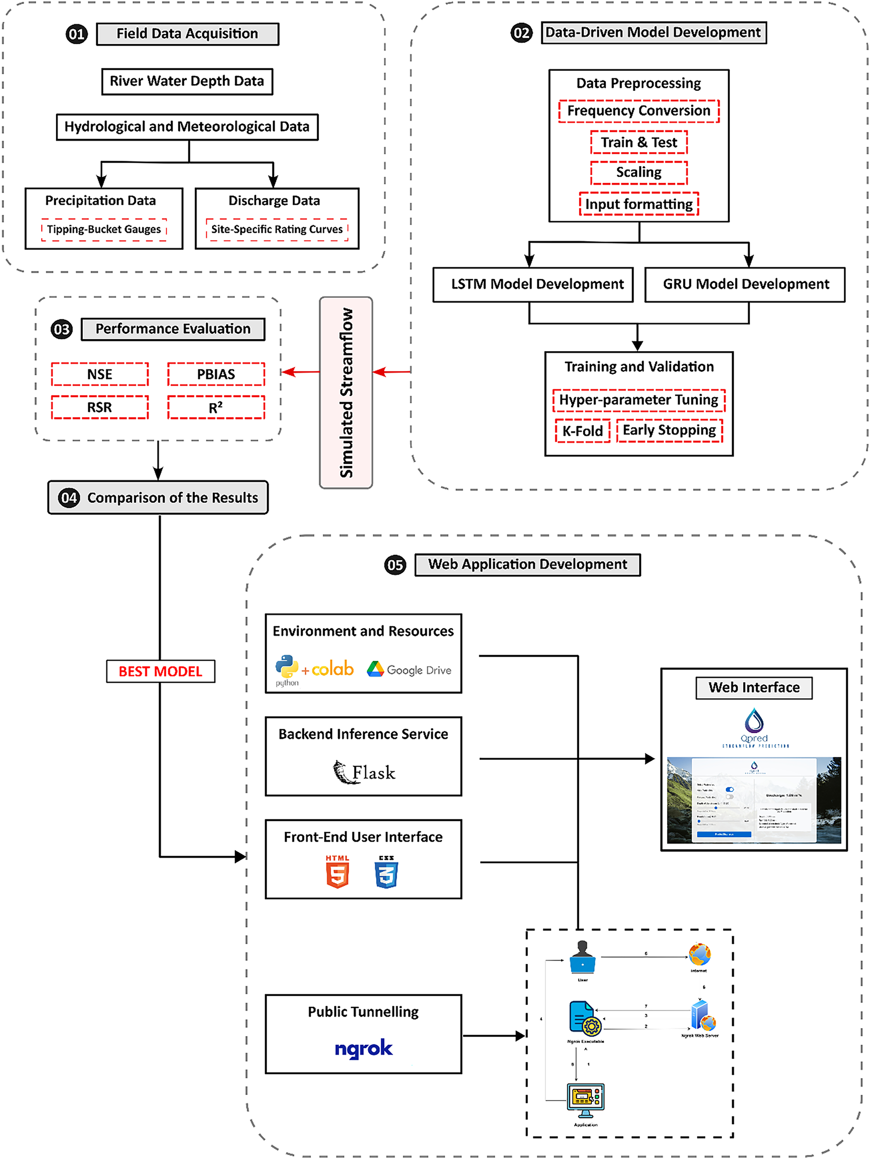
Figure 1: Flowchart of the research methodology

2.1 Study Area

The Aglar watershed, which is about 305 km2 in size, located in the Tehri Garhwal district of Uttarakhand, is positioned between latitudes 30°25′ and 30°30′ and longitudes 77°58′ and 77°18′ (refer to Fig. 2). The watershed comprises three sub-adjoining watersheds: Upper Aglar, Paligaad, and Balganga, with data collection conducted at the outlets of the Aglar (Upper) (hereafter Algar) and Paligaad sub-watersheds. The southern section of the watershed exhibits undulating topography with minimal to no vegetation, whereas the northern section is renowned for its perennial streams, valleys, and peaks. The watershed’s complex topography, which drains into the Yamuna River, varies in elevation from 715 to 3015 m above mean sea level (MSL). Paligaad, one of the primary sub-watersheds, is characterized by similar elevational gradients and monsoon-dominated hydrology, with monitoring stations established at its outlet to capture streamflow dynamics. Approximately 70% of the annual rainfall occurs during the South-West monsoon season (mid-June to mid-September), averaging 1800 mm. The area experiences between 70 and 80 wet days annually, with rainfall distributed across the monsoon, winter, and summer seasons. Although the region is endowed with ample water resources and forest cover, the primary concern lies in the current unscientific exploitation of these resources, thereby posing significant challenges to the sustainability of ecosystem services.

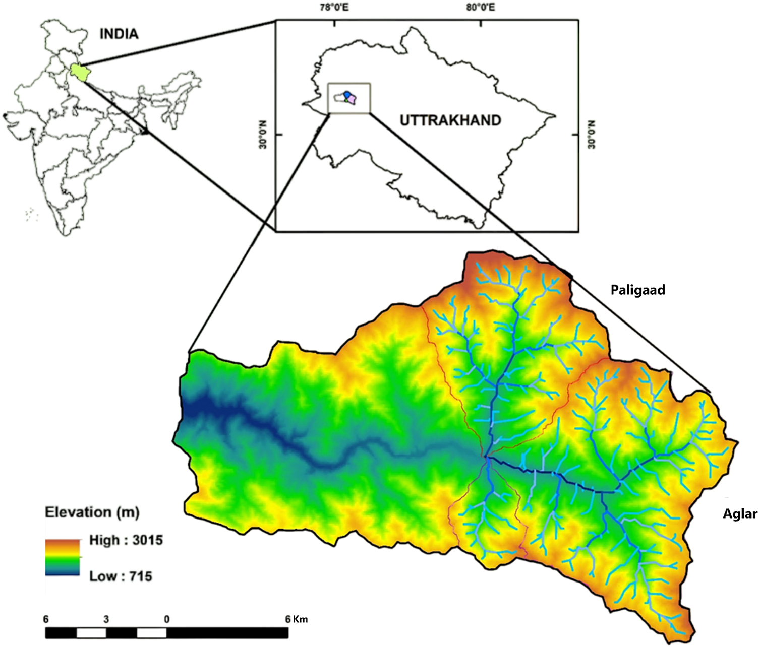
Figure 2: Study area selected for the data collection

2.2 Data Acquisition

Accurate monitoring of hydro-meteorological parameters is essential in vulnerable catchments such as the Aglar watershed due to the increasing frequency and severity of hydro-meteorological disasters in recent years, including flash floods, landslides, and extreme rainfall events. The Aglar watershed was entirely ungauged until recently, despite being affected by numerous natural hazards. To address this data deficiency and to enhance understanding of the temporal and spatial variability of stream discharge and rainfall, a comprehensive hydro-meteorological monitoring network was established. An Odyssey tipping bucket rain gauge and RainWise logger were employed as depicted to procure high-resolution rainfall measurements, enabling precise documentation of rainfall intensity and temporal distribution.

To record hourly variations in water levels, two Odyssey water level recorders were also installed at the outlets of the two sub-watersheds (Aglar and Paligaad). Site-specific rating curve equations, derived through field calibration, were employed to convert these river water depth measurements into discharge values. The initial baseline dataset for this watershed was established by systematically recording daily hydrometeorological parameters from 2014 to 2016. This observational dataset is crucial for the development of the hydrological model and enhances disaster risk reduction efforts in this highly sensitive and ungauged region, as well as fostering a better understanding of the watershed’s hydrological response under changing climatic conditions. Fig. 3 presents a few photographs taken during the field survey.

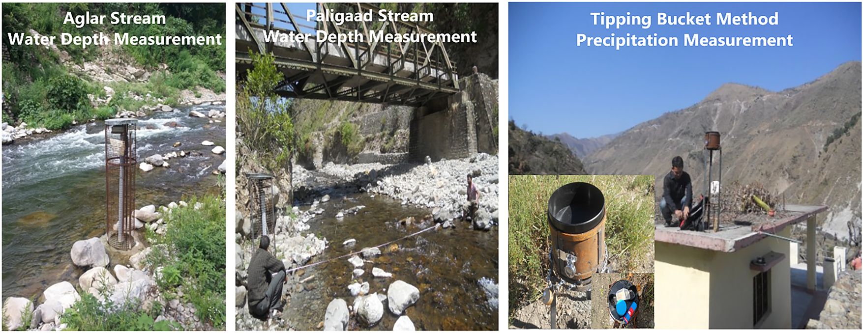
Figure 3: Field photographs during the data collection in Aglar and Paligaad streams

2.3 Data-Driven Model Development

2.3.1 Data Preprocessing

Prior to the analysis, the dataset underwent a two-stage preprocessing workflow. First, outlier detection was performed using the Z-score criterion, followed by the identification of missing values. However, due to meticulous documentation of the records, no significant outliers or missing values were found within the dataset; the authors then proceeded to aggregate the hourly observations into daily values for subsequent model development.

LSTM and GRU models were developed to forecast daily streamflow with a lead time of one day, utilising a 90-day window of historical precipitation and water depth inputs. The chronological sequence of observations was divided into a training period, comprising approximately 70%, and a validation period, comprising approximately 30%. The total number of data instances was approximately 890 in Aglar and 920 in Paligaad. Due to this limited sample size, the authors did not provide a separate test set; instead, all model selection and performance evaluation were conducted based on the validation set results, thereby optimizing the use of available data for both model fitting and unbiased assessment. All input data were subsequently scaled using a robust scaling method to ensure smooth training while mitigating the influence of extreme values. Scaling parameters were derived from the training data and subsequently applied to the validation data to prevent any data leakage. Finally, the data were reshaped into three-dimensional tensors of appropriate shape ([nsamples,ntimesteps,nfeatures]) to meet the input data structure requirements of both recurrent architecture and subsequent processing stages before being fed into the models.

2.3.2 LSTM Model and Development

LSTM networks, proposed by Hochreiter and Schmidhuber [16], possess three nonlinear gating mechanisms, including input, forget, and output gates, as illustrated in Fig. 4.

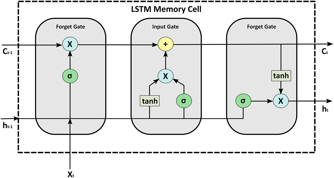
Figure 4: LSTM memory cell, with key components including activation functions, memory cell states, hidden states, and vector operations

These gates regulate information flow through a dedicated memory cell, which functions as a neuron with a self-recurrent connection. These networks specialise in managing long-term dependencies by determining which portion of the previous state of the cell should be retained or discarded due to the integration of the forget gate, making it more suitable for hydrological modelling compared to traditional RNN architecture. The forget gate output (ft) is computed as follows,

ft=σ(Wf[ht−1,xt]+bf)(1)

where σ is the sigmoid activation function, ht−1 is the previous hidden state, xt is the current input and Wf, bf are the gates trainable weights and bias. Then the input gate determines which new information to write into the cell using two steps as follows,

it=σ(Wi[ht−1,xt]+bi)(2)

Ct∼=tanh⁡(Wc[ht−1,xt]+bc)(3)

here, it controls the information addition from Ct∼ to the cell state. Wi, Wc, bi and bc are the trainable parameters. The new cell state formed as follows,

Ct=ft⊙Ct−1+it⊙Ct∼(4)

Finally, the output gate (ot) determines what part of the cell state to expose as the new hidden state (ht) as follows,

ot=σ(Wo[ht−1,xt]+bo)(5)

ht=ot⊙tanh⁡(Ct)(6)

Therefore, using this model, we developed and evaluated three LSTM-based architectures, including a vanilla LSTM (single-layer LSTM) (Fig. 5a), a stacked LSTM [27] (Fig. 5b), and a bidirectional LSTM [28] (Fig. 5c) to predict the daily streamflow. Precipitation and water depth were used as inputs, while discharge served as the target variable. However, we excluded the lagged features as inputs to prevent autocorrelation and to ensure that the models learned hydrological responses driven solely by the observed data, thereby enhancing physical interpretability and transferability, as the author’s focus was on developing a practical web-based application.

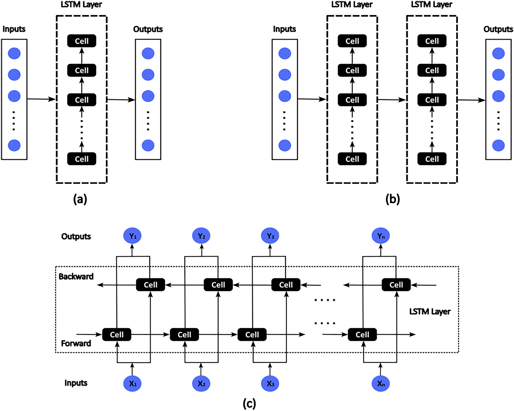
Figure 5: LSTM models utilized in the study: (a) Vanilla LSTM; (b) Stacked-LSTM; (c) Bi-LSTM

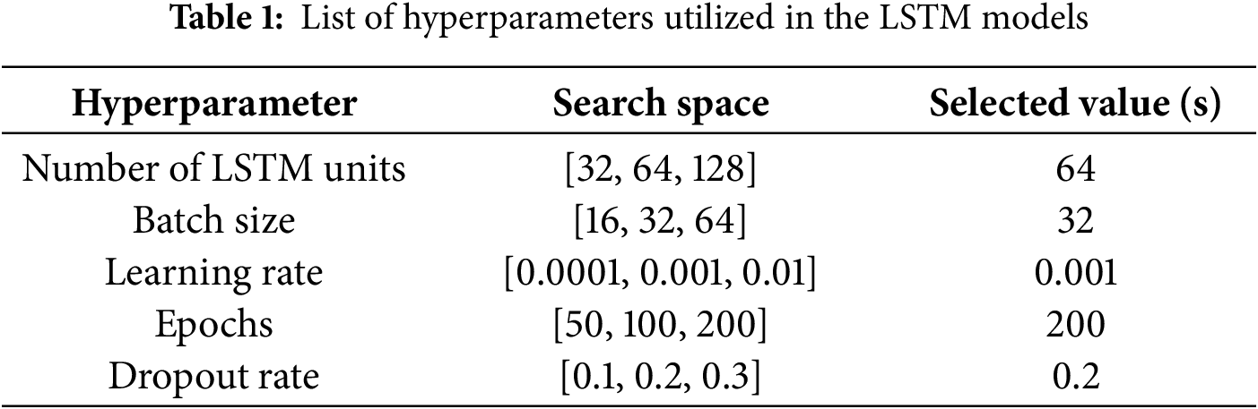
Due to the moderate size of the data, this study employed several strategies, including dropout regularization, early stopping, TimeSeriesSplit K-fold cross-validation (K = 5), and meticulous hyperparameter tuning to prevent overfitting and ensure robust generalization during the validation phase. A grid search approach was utilised to perform hyperparameter tuning over a bounded set of values, as depicted in Table 1, informed by prior hydrological and time series studies as well as preliminary experiments. The Adam optimizer was used as the standard optimizer for this study, owing to its adaptive learning rate capabilities and robust convergence behaviour in similar forecasting applications.

2.3.3 GRU Model and Development

GRU networks, introduced by Cho et al. [21], simplify the LSTM architectures by merging the forget gate and the input gate into a single update gate and combining the cell state with the hidden state, as illustrated in Fig. 6. The primary gating mechanisms in a GRU are the reset gate (rt) and the update gate (Zt). These gates regulate the flow of information directly into the hidden state, enabling the network to capture long-term dependencies with fewer parameters than a traditional LSTM. The update gate controls the retention of the information from the previous hidden state (ht−1) and the reset gate determines the new information that should be added to the previous memory as follows.

Zt=σ(Wz[ht−1,xt]+bz)(7)

rt=σ(Wr[ht−1,xt]+br)(8)

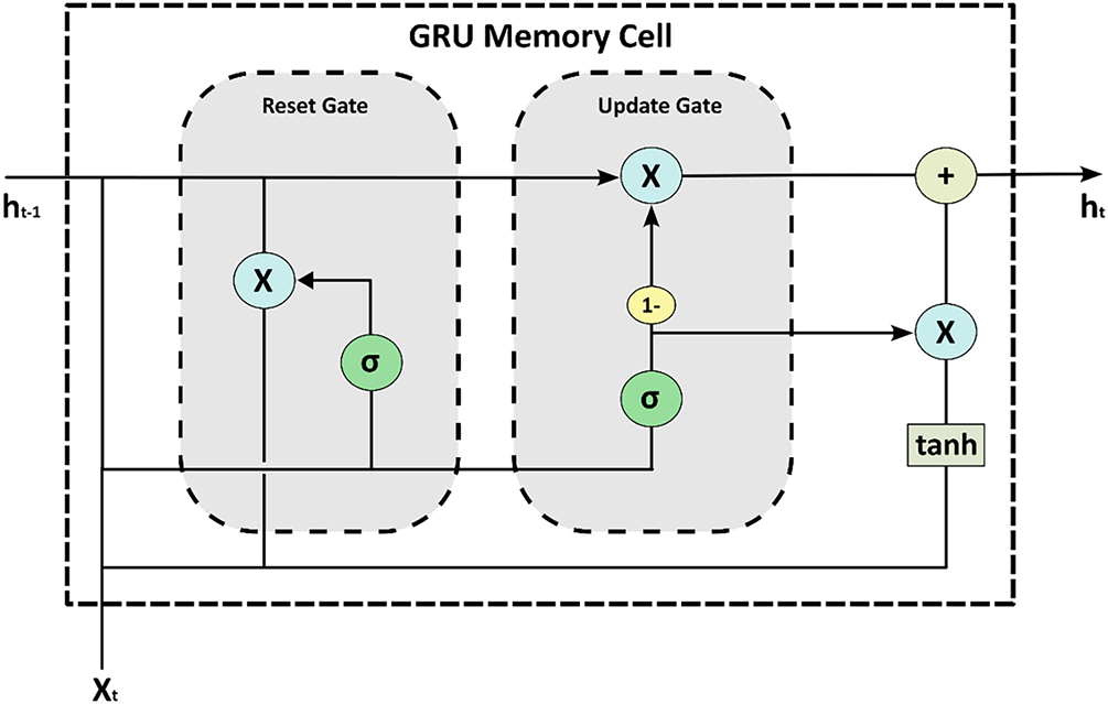
Figure 6: GRU memory cell, with two gates, activation functions, and vector operations

Then, as shown in Eq. (9), a candidate hidden state (ht∼) is then computed using the reset gate to forget the parts of the previous state.

ht∼=tanh⁡(Wh[rt⊙ht−1,xt]+bh)(9)

Finally, the new hidden state (ht) is formed using a linear interpolation between the previous state and the candidate state, governed by the update gate as follows,

ht=(1−Zt)⊙ht−1+Zt⊙ht∼(10)

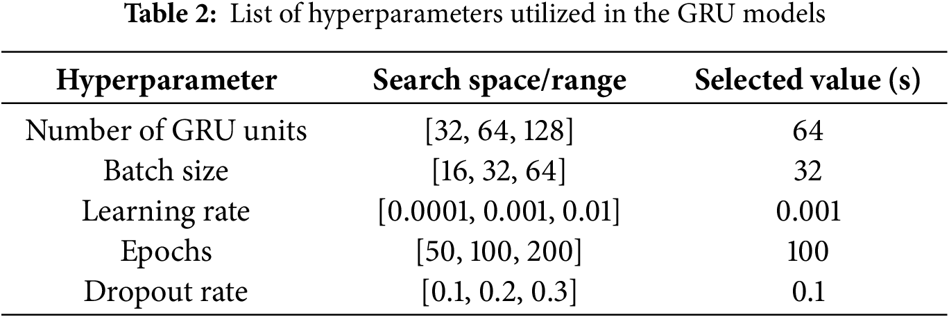
Similar data structures, settings, and strategies were employed to model the GRU, analogous to those used in the LSTMs. Table 2 presents the parameters and their respective search space utilised in grid search, along with the selected values, comparable to the LSTM modelling.

2.4 Performance Evaluation

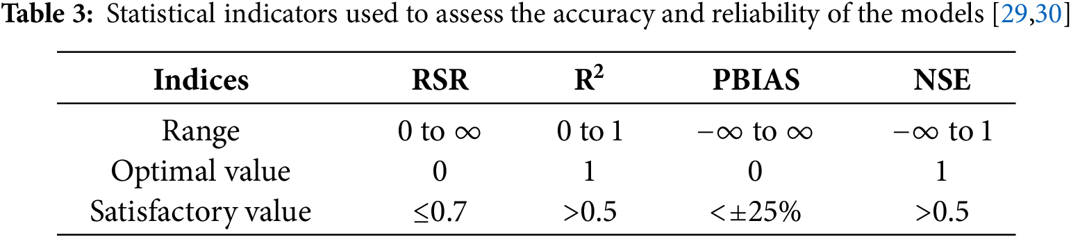
The performance of each model was evaluated using four statistical metrics commonly employed for hydrological model assessment: Nash-Sutcliffe Efficiency (NSE), the Root-Mean-Square-Error-Standard-Deviation Ratio (RSR), Percentage Bias (PBIAS), and the Coefficient of Determination (R2), as outlined in Table 3. The range of each statistical indicator, along with optimal and satisfactory values, is also illustrated, while Eqs. (11)–(14) provide the mathematical expressions utilised for the calculations of each indicator.

R2=[∑i(Qobs,i−Q¯obs)(Qsim,i−Q¯sim)]2∑i(Qobs,iQ¯obs)2∑i(Qsim,i−Q¯sim)2(11)

NSE=1−∑i(Qobs−Qsim)i2∑i(Qobs,i−Q¯obs)2(12)

RSR=∑i=1n(Qobs−Qsim)i2∑i=1n(Qobs,i−Q¯sim)2(13)

PBIAS=100×∑i=1n(Qobs−Qsim)i∑i=1nQobs,i(14)

where Qsim,i and Qobs,i represent observed and predicted discharge at time step i, Qsim and Qobs are their respective means, and n is the sample size.

2.5 Web Application Development

QPred operates as an on-demand inference system where users manually input current hydrometeorological conditions to receive one-day-ahead discharge predictions. The system utilizes pre-trained LSTM/GRU models that remain static after deployment and do not perform online learning. This manual-input approach was chosen to ensure accessibility in data-scarce regions lacking automated telemetry infrastructure, while maintaining the demonstration of how deep learning models can be operationally deployed through lightweight web platforms. The QPred web application development workflow encompasses four steps: environment and resources, backend inference service, front-end user interface, and public tunnelling and security.

2.5.1 Environment and Resources

Google Colab was selected as the primary development and execution environment due to its on-demand computing resources (GPU/TPU) and cost-free environment, despite its ephemeral runtime and the lack of a routable public IP for an isolated environment. All Python dependencies, including Flask, scientific libraries, and model-related packages, were installed, and their versions were fixed prior to development to ensure reproducibility across sessions. Pretrained models and other auxiliary assets were persisted in Google Drive. The notebook’s mounted drive was initialised, file integrity was verified, and these artefacts were loaded into memory to minimize inference latency.

2.5.2 Backend Inference Service

Flask served as the backend microframework, exposing model inference as Hypertext Transfer Protocol (HTTP) Uniform Resource Locator (URLs). The inputs were developed to be constrained with range sliders to ensure the server received only in-range values, thereby minimizing the need for server-side validations. The range was established based on the dataset’s minimum and maximum values. Each request then scaled utilizing the same scaling process used during training, invoked the LSTM/GRU models for prediction, and post-processed outputs into discharge units. This process was handled sequentially due to the single-process kernel architecture of Colab and was adequate for this project.

2.5.3 Front-End User Interface

The front-end user interface was generated using render_template_string. This Flask function renders templates directly from strings within the code. This approach avoided separate static HyperText Markup Language (HTML) files and enabled rapid iteration within the notebook. The interface collected rainfall and stream depth inputs for the Aglar and Paligaad watersheds and displayed predicted discharge values with other relevant information in real time. The application was designed to be stateless, with each HTTP request containing all necessary inputs, making it simplified but requiring resubmission of preferences on each iteration.

2.5.4 Public Tunnelling

Public tunneling was accomplished through Ngrok, as depicted in Fig. 7, which illustrates the mechanism of the Ngrok tunneling process. (1) The web application was first started on a cloud environment (Google Colab); (2) With the Ngrok executable, a secure tunnelling process was initiated via a designated port (port 5000), connecting to the localhost application; (3) Upon successful connection, Ngrok generated a temporary public HTTPS URL that pointed directly to the local Flask server; (4) This URL was then shared with users, enabling them to access the application through their web browsers, even though it was hosted within a private Colab environment; (5) The application was accessed by end users through the provided public link over the internet; (6) When a user submitted a request using the shared link, the request first reached Ngrok’s global edge servers, as the URL uses an ngrok.com subdomain; (7) Ngrok then mapped the public URL to the local address by establishing a reverse proxy tunnel, securely forwarding incoming traffic to the Flask server operating on localhost; (8) Finally, the forwarded request reached and interacted with the local application.

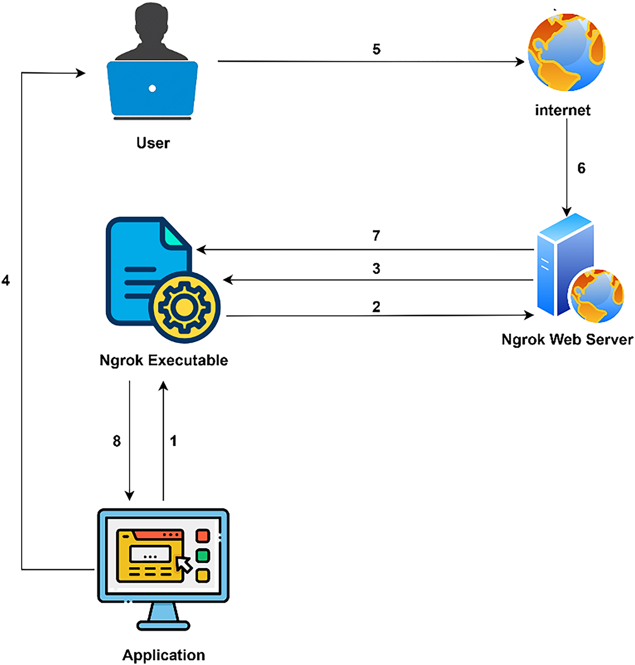
Figure 7: Ngrok mechanism for tunneling a local web application to the internet

This process was maintained over a persistent connection utilizing HTTP or WebSockets to ensure rapid, real-time communication. Each request from the client was securely routed through Ngrok’s infrastructure, then to the Colab-hosted server, and the response was sent back along the same tunnel to the user. Ngrok also applied transport layer security (TLS) encryption by default, ensuring that all data transmitted between the client and the local server is encrypted. The tunnel was temporary and automatically terminated when the Colab session ended, adding a layer of security and making it ideal for temporary demos and testing purposes [31].

3  Results and Discussions

3.1 Deep Learning Models Performance

3.1.1 Hydrographs Evaluation

The hydrographs presented for the Aglar and Paligaad river basins illustrate the temporal dynamics of observed and simulated streamflow using the DL models utilized in Fig. 8. For the Aglar watershed (refer to Fig. 8a), all four models exhibit a strong capacity to replicate the overall shape and timing of the observed hydrograph during both calibration and validation periods. Although not notably depicted, the bidirectional LSTM and GRU models appear to follow observed discharge patterns with slightly higher fidelity during peak and low flow events. The vanilla and stacked LSTM models also demonstrate consistent performance, albeit with marginal underestimation of peak magnitudes in some instances. During the validation phase, all models sustain reasonable predictive performance beyond the calibration window, demonstrating strong generalization. However, minor deviations occurred, primarily during peak periods, which are inherently challenging to simulate due to abrupt hydrological responses and non-stationarities in rainfall-runoff processes.

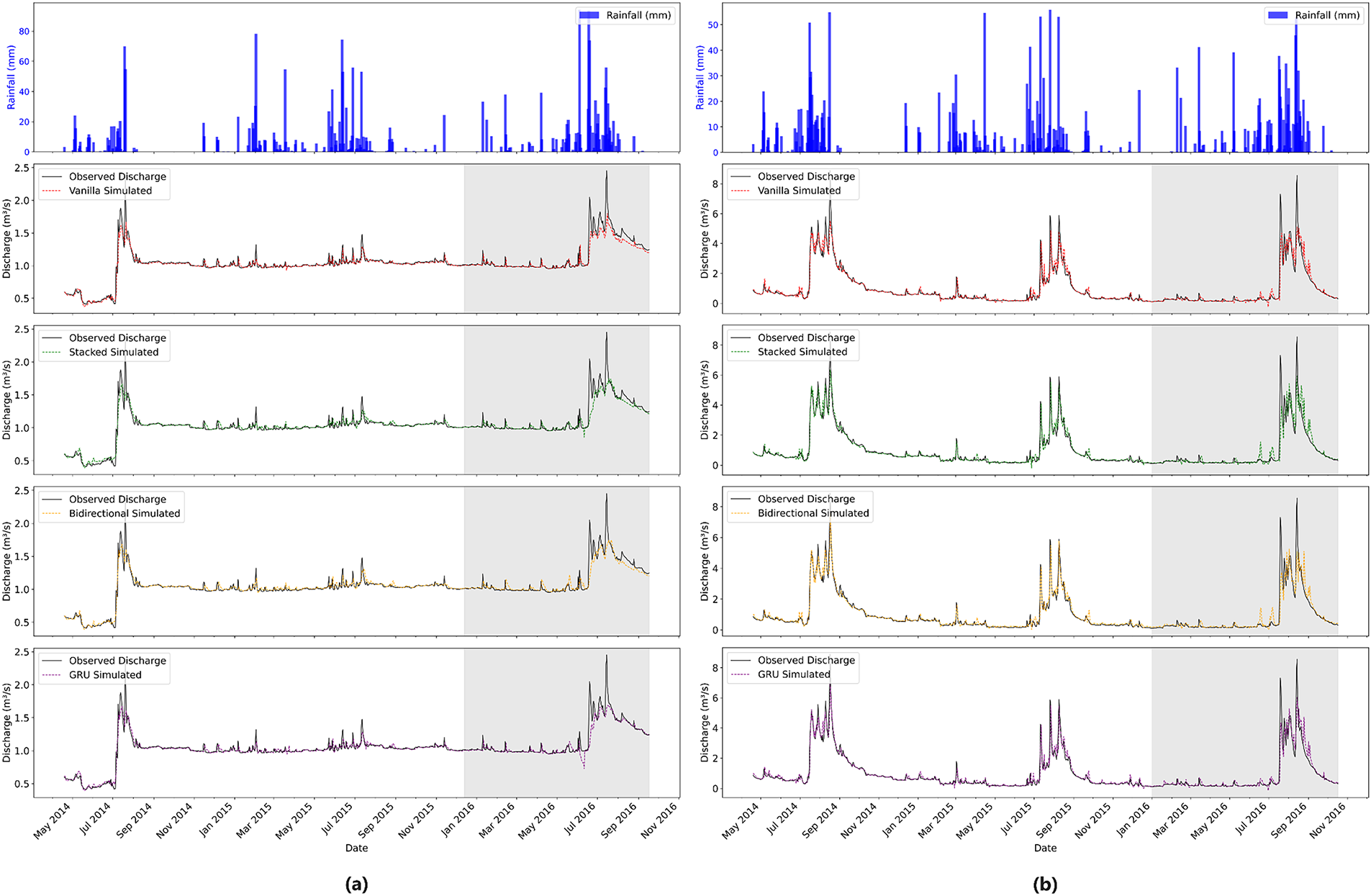
Figure 8: Comparison of observed and simulated streamflow discharge in data-driven models at Aglar (a) and Paligaad (b). Grey colour represents the validation period

In the Paligaad watershed (refer to Fig. 8b), characterized by generally higher flow magnitudes and more pronounced peak events, the models accurately capture these dynamics. The similarity between observed and simulated hydrographs by the bidirectional LSTM and GRU models during calibration and validation periods further underscores their strength in modeling complex temporal dependencies and flow heterogeneity. However, it is noteworthy that the vanilla LSTM model struggles to capture the peak flows in comparison to other models during the calibration phase. The validation period demonstrates sustained predictive capability, with the models effectively simulating both low and high flows, although the accuracy was not comparable to that of the calibration phase. Nevertheless, the accuracy remains at a high level, establishing the robustness of these models in water resources management and flood forecasting, where models are expected to perform reliably under various contexts.

3.1.2 Statistical Evaluation

Table 4 presents the statistical evaluation results comparing the predictive performance of the data-driven models used for streamflow forecasting in the Aglar and Paligaad river basins. In the Aglar watershed, all four models demonstrated strong predictive capabilities during the calibration phase. The bidirectional LSTM and GRU models slightly outperformed the vanilla and stacked LSTM models, with the highest R2 and NSE values of 0.92, indicating an excellent fit between observed and simulated streamflow. The Root Mean Square Error (RMSE) values were minimal for the bidirectional LSTM and GRU models, each registering at 0.06. Additionally, the RSR values were also lowest for the bidirectional LSTM at 0.28, thereby indicating superior calibration accuracy. The stacked LSTM and vanilla LSTM models exhibited comparable performance, with R2 and NSE values of 0.91 and RSR values of 0.30.

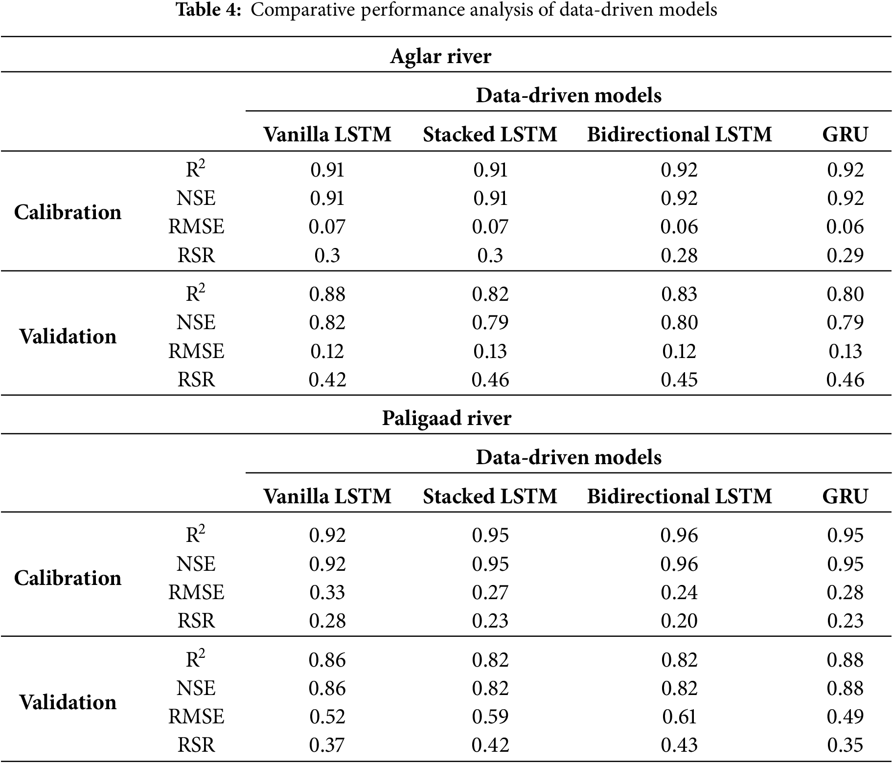
Validation results demonstrated a moderate decline in model performance, which is anticipated when evaluated on unseen data. The vanilla LSTM maintained relatively strong predictive capabilities, with an R2 of 0.88 and NSE of 0.82, and recorded the lowest RMSE (0.12) among the models, indicating superior generalization. The bidirectional LSTM also preserved robust accuracy (R2 = 0.83, NSE = 0.80), albeit with a marginally higher RMSE (0.12). Conversely, the stacked LSTM and GRU models exhibited a considerable reduction in validation performance, with R2 values of 0.82 and 0.80, NSE approximately 0.79, and slightly elevated RMSEs (0.13). The RSR values increased across all models, ranging from 0.42 to 0.46, reflecting a decrease in prediction precision but maintaining satisfactory overall validation performance.

In the Paligaad watershed, the results of model calibration demonstrated notable strength overall, with the bidirectional LSTM attaining the highest R2 (0.96) and NSE (0.96), thereby indicating an excellent model fit. The GRU and stacked LSTM models also exhibited commendable performance, with R2 and NSE values approximately 0.95, whereas the vanilla LSTM recorded slightly lower values, R2 and NSE of 0.92. The RMSE was minimised for the bidirectional LSTM at 0.24, complemented by the lowest RSR of 0.2, signifying superior accuracy and diminished error during the calibration phase.

During the validation phase, although the performance of all models declined across all metrics, the GRU model exhibited notable generalization capabilities relative to the others, achieving the highest R2 and NSE values of 0.88, as well as the lowest (0.49) and RSR (0.35). The vanilla LSTM also maintained commendable validation performance (R2 and NSE = 0.86), with a moderate RMSE (0.52) and RSR (0.37). The stacked LSTM and bidirectional LSTM showed somewhat reduced validation efficacy (R2 and NSE approximately 0.82), accompanied by increased RMSE values (0.59 and 0.61) and RSR between 0.42 and 0.43, suggesting a relative decline in predictive accuracy for unseen data.

In both watersheds, all models demonstrated robust calibration performance, with the bidirectional LSTM model generally providing the best fit to the training data. However, validation results highlight variability in generalization capabilities, where the vanilla LSTM and GRU models often outperformed more complex architectures such as stacked and bidirectional LSTM in unseen conditions, particularly for the Parligaad watershed. This suggests that simpler or gated recurrent structures may offer a better balance between model complexity and generalization in streamflow prediction in certain contexts.

3.1.3 Scatterplots Evaluation

Scatterplots comparing observed and simulated streamflow during both calibration and validation phases for the DL models are presented for the Aglar and Paligaad watersheds in Fig. 9. As illustrated in Fig. 9a, during calibration, the scatterplots for all models show data points closely clustered around the 1:1 line, indicating strong agreement between observed and predicted streamflow in the Aglar watershed. The bidirectional LSTM and GRU models display slightly tighter clustering and less scatter, highlighting their higher accuracy and better fit during this phase. The vanilla and stacked LSTM models also exhibit good alignment but with marginally more dispersion.

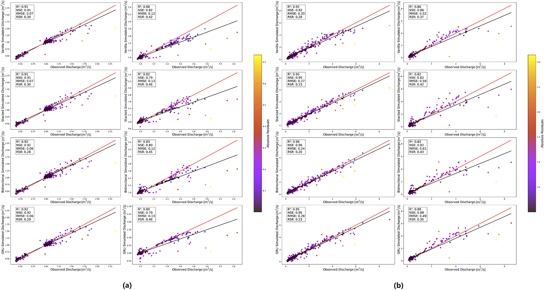
Figure 9: Scatterplots between observed and simulated streamflow for (a) Aglar and (b) Paligaad. Each plot (a,b) is divided into Calibration (left side) and Validation (right side). The best-fit line and bisector line are depicted in black and red, respectively

During the validation phase, an anticipated increase in dispersion around the bisector line is observed across all models, reflecting the inherent challenges associated with predicting unseen data. The vanilla LSTM exhibits relatively less dispersion and superior overall alignment, indicating more reliable generalization capability. Other models demonstrate slightly greater variability, particularly at higher discharge values, where deviations from the ideal line are more apparent, suggesting potential difficulties in accurately capturing the streamflow dynamics.

In the Paligaad watershed (Fig. 9b), calibration scatterplots reveal excellent predictive performance across all models, similar to the Aglar. Points are tightly aligned along the 1:1 line with minimal scatter, particularly for the bidirectional and stacked LSTM and GRU models, which demonstrate the strongest fit. The vanilla LSTM model also exhibits strong performance, with slightly greater spread but maintaining close conformity. During validation, increased scatter is observed across all models, indicating a decline in prediction accuracy on independent data similar to the pattern observed in the Aglar watershed. The GRU and vanilla LSTM models exhibit comparatively better consistency, with less deviation from the bisector line, while the stacked and bidirectional LSTM models show higher dispersion, especially at larger discharge values. It’s evident that the simpler architectures maintain more robust generalisation within this specific context, as suggested in the statistical evaluation.

3.2 DL Model Intergrated Web Application

Fig. 10 illustrates the QPred web-based application interface, which adheres to a straightforward two-step workflow: (i) users provide specific inputs, and (ii) receive discharge predictions in real time. Initially, the left-hand panel offers concise instructions, and following the ‘predict discharge’ action, the right-hand panel dynamically displays the model output and metadata, maintaining a single-page, low-latency interaction.

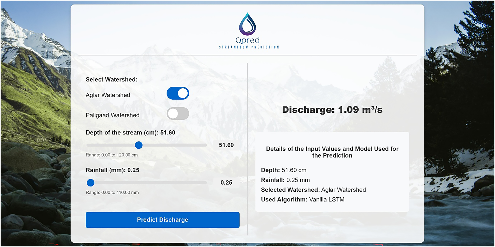
Figure 10: QPred web application interface

3.2.1 User Interface-Input Features

The input pane collects the predictors required by the models, including observed stream water depth (cm) and precipitation (mm), along with the watershed selector (Aglar or Paligaad). To prevent invalid entries and to reflect the training domain, both variables are constrained via slider buttons, whose ranges are defined based on respective watershed datasets as discussed in the development section. The predefined ranges are: 0–120 cm for depth and 0–110 mm for rainfall in the Aglar watershed, and 0–100 cm for depth and 0–65 mm for rainfall in the Paligaad watershed. Therefore, the slider buttons allow users to adjust the input values, and users can view the current input values at the moment of adjusting the slider before proceeding.

3.2.2 User Interface-Prediction Output and Details

The output pane succinctly presents the hydrological model results and other pertinent information. The primary output, discharge, is articulated in cubic meters per second (m3/s) in accordance with user inputs, facilitating immediate comprehension of streamflow conditions. Additionally, the system displays the input information, including the selected watershed, depth, and rainfall, and specifies the conventional machine learning algorithm employed for prediction as supplementary details. This enables users to cross-reference the prediction data. The default models, vanilla LSTM for the Aglar watershed and GRU for the Paligaad watershed, are automatically selected during the watershed selection process. These details enhance transparency and foster trust in the system, thereby allowing users to evaluate the reliability of the predictions.

4  Conclusion and Recommendations

This study introduced QPred, a regional, cost-effective, and lightweight web application designed to operationalise DL models for daily streamflow forecasting. It demonstrates a comprehensive workflow from field data acquisition to end-user deployment. High-resolution rainfall measurements obtained via tipping bucket gauges and loggers, along with river water depth observations converted to discharge through site-specific rating curves, provided a daily dataset (2014–2016) for the Aglar and Paligaad Himalayan watersheds. Four RNN architectures, including vanilla, stacked, and bidirectional LSTMs, as well as a GRU, were trained and evaluated using NSE, R2, PBIAS, and RSR. Performance demonstrated watershed-specific effectiveness, with the vanilla LSTM proving most effective in Aglar, while the GRU achieved the highest validation accuracy in Paligaad. These optimal models were subsequently integrated into QPred. The application was developed utilising a lightweight stack comprising Google Colab, Flask, Google Drive, and Ngrok, thereby providing advanced forecasting capabilities through a web browser interface without necessitating specialized infrastructure or conventional machine learning expertise from end users.

Although QPred offers a valuable baseline, there exist multiple avenues for enhancement. Presently, the model relies on two predictors: precipitation and river water depth. Incorporating additional variables such as temperature, humidity, and wind speed could potentially improve the accuracy and robustness of the prediction. Additionally, future research may explore hybrid or physics-informed DL models to improve current predictive accuracy and further integrate hydrological principles. Implementing these enhancements alongside adopting and testing for other watersheds assists in developing the QPred application into a robust, versatile platform for DL-based streamflow prediction, benefiting hydrological practitioners and relevant authorities.

Acknowledgement: Not applicable.

Funding Statement: The authors received no specific funding for this study.

Author Contributions: Randika K. Makumbura: writing—original draft, visualization, software, resources, methodology, investigation, formal analysis, data curation. Hasanthi Wijesundara: writing—original draft, visualization, data curation. Hirushan Sajindra: writing—original draft, visualization, software, resources, methodology, investigation, formal analysis, data curation. Upaka Rathnayake: supervision, validation, project administration, conceptualization, writing—review & editing. Vikram Kumar: supervision, validation, writing—review & editing. Dineshbabu Duraibabu: supervision, validation, writing—review & editing. Sumit Sen: supervision, validation, writing—review & editing. All authors reviewed the results and approved the final version of the manuscript.

Availability of Data and Materials: Data and Material will be made available on reasonable request.

Ethics Approval: Not applicable.

Conflicts of Interest: The authors declare no conflicts of interest to report regarding the present study.

References

1. Dalkilic HY, Kumar D, Samui P, Dixon B, Yesilyurt SN, Katipoğlu OM. Application of deep learning approaches to predict monthly stream flows. Environ Monit Assess. 2023;195(6):705. doi:10.1007/s10661-023-11331-5. [Google Scholar] [PubMed] [CrossRef]

2. Vatanchi SM, Etemadfard H, Maghrebi MF, Shad R. A comparative study on forecasting of long-term daily streamflow using ANN, ANFIS, BiLSTM and CNN-GRU-LSTM. Water Resour Manag. 2023;37(12):4769–85. doi:10.1007/s11269-023-03579-w. [Google Scholar] [CrossRef]

3. Kumar V, Unal S, Bhagat SK, Tiyasha T. A data-driven approach to river discharge forecasting in the Himalayan region: insights from Aglar and Paligaad rivers. Results Eng. 2024;22:102044. doi:10.1016/j.rineng.2024.102044. [Google Scholar] [CrossRef]

4. Ali Sit M, Demiray BZ, Demir I. A systematic review of deep learning applications in streamflow data augmentation and forecasting. EarthArXiv. 2022. doi:10.31223/X5HM08. [Google Scholar] [CrossRef]

5. Workneh HA, Jha MK. Utilizing deep learning models to predict streamflow. Water. 2025;17(5):756. doi:10.3390/w17050756. [Google Scholar] [CrossRef]

6. Shah AI, Sen S, Mishra A. Hydrological modeling of the paligad watershed (India) using HSFP model. Int J Environ Clim Change. 2019;2019:217–28. doi:10.9734/ijecc/2019/v9i430109. [Google Scholar] [CrossRef]

7. Gao S, Huang Y, Zhang S, Han J, Wang G, Zhang M, et al. Short-term runoff prediction with GRU and LSTM networks without requiring time step optimization during sample generation. J Hydrol. 2020;589:125188. doi:10.1016/j.jhydrol.2020.125188. [Google Scholar] [CrossRef]

8. Ougahi JH, Rowan JS. Enhanced streamflow forecasting using hybrid modelling integrating glacio-hydrological outputs, deep learning and wavelet transformation. Sci Rep. 2025;15:2762. doi:10.1038/s41598-025-87187-1. [Google Scholar] [PubMed] [CrossRef]

9. Singh D, Vardhan M, Sahu R, Chatterjee D, Chauhan P, Liu S. Machine-learning- and deep-learning-based streamflow prediction in a hilly catchment for future scenarios using CMIP6 GCM data. Hydrol Earth Syst Sci. 2023;27(5):1047–75. doi:10.5194/hess-27-1047-2023. [Google Scholar] [CrossRef]

10. Talukdar S, Pal S, Shahfahad N, Naikoo MW, Parvez A, Rahman A. Trend analysis and forecasting of streamflow using random forest in the Punarbhaba River basin. Environ Monit Assess. 2022;195(1):153. doi:10.1007/s10661-022-10696-3. [Google Scholar] [PubMed] [CrossRef]

11. Essam Y, Huang YF, Ng JL, Birima AH, Ahmed AN, El-Shafie A. Predicting streamflow in Peninsular Malaysia using support vector machine and deep learning algorithms. Sci Rep. 2022;12(1):3883. doi:10.1038/s41598-022-07693-4. [Google Scholar] [PubMed] [CrossRef]

12. Tongal H, Booij MJ. Simulation and forecasting of streamflows using machine learning models coupled with base flow separation. J Hydrol. 2018;564:266–82. doi:10.1016/j.jhydrol.2018.07.004. [Google Scholar] [CrossRef]

13. Tang Z, Zhang J, Hu M, Ning Z, Shi J, Zhai R, et al. Improving streamflow forecasting in semi-arid basins by combining data segmentation and attention-based deep learning. J Hydrol. 2024;643:131923. doi:10.1016/j.jhydrol.2024.131923. [Google Scholar] [CrossRef]

14. Hadiyan PP, Moeini R, Ehsanzadeh E. Application of static and dynamic artificial neural networks for forecasting inflow discharges, case study: sefidroud Dam reservoir. Sustain Comput Inform Syst. 2020;27:100401. doi:10.1016/j.suscom.2020.100401. [Google Scholar] [CrossRef]

15. Le XH, Nguyen DH, Jung S, Yeon M, Lee G. Comparison of deep learning techniques for river streamflow forecasting. IEEE Access. 2021;9:71805–20. doi:10.1109/access.2021.3077703. [Google Scholar] [CrossRef]

16. Hochreiter S, Schmidhuber J. Long short-term memory. Neural Comput. 1997;9(8):1735–80. doi:10.1162/neco.1997.9.8.1735. [Google Scholar] [PubMed] [CrossRef]

17. Makumbura RK, Manatunge J, Rathnayake U. Bridging data-driven and process-based approaches for hydrological modeling in the tropics: insights from the Kelani River Basin, Sri Lanka. Results Eng. 2025;27:105975. doi:10.1016/j.rineng.2025.105975. [Google Scholar] [CrossRef]

18. Kratzert F, Klotz D, Brenner C, Schulz K, Herrnegger M. Rainfall–runoff modelling using long short-term memory (LSTM) networks. Hydrol Earth Syst Sci. 2018;22(11):6005–22. doi:10.5194/hess-22-6005-2018. [Google Scholar] [CrossRef]

19. Li B, Li R, Sun T, Gong A, Tian F, Ali Khan MY, et al. Improving LSTM hydrological modeling with spatiotemporal deep learning and multi-task learning: a case study of three mountainous areas on the Tibetan Plateau. J Hydrol. 2023;620:129401. doi:10.1016/j.jhydrol.2023.129401. [Google Scholar] [CrossRef]

20. Wang K, Bertoli G, Cheng S, Schröter K, Caporali E, Piggott MD, et al. AI-empowered latent four-dimensional variational data assimilation for river discharge forecasting. IEEE J Sel Top Appl Earth Obs Remote Sens. 2025;18:24676–89. doi:10.1109/jstars.2025.3611136. [Google Scholar] [CrossRef]

21. Cho K, van Merrienboer B, Bahdanau D, Bengio Y. On the properties of neural machine translation: encoder-decoder approaches. arXiv:1409.1259. 2014. [Google Scholar]

22. Ajah O, Afolayan AH, Akinwonmi AE. A comparative study of long short-term memory and gated recurrent units for forecasting rainfall: a case study of Nigeria. Int J Appl Inf Syst. 2024;12(46):15–24. doi:10.5120/ijais2025451987. [Google Scholar] [CrossRef]

23. Chung J, Gulcehre C, Cho K, Bengio Y. Empirical evaluation of gated recurrent neural networks on sequence modeling. arXiv:1412.3555. 2014. [Google Scholar]

24. Karamvand A, Hosseini SA, Ali Azizi S. Enhancing streamflow simulations with gated recurrent units deep learning models in the flood prone region with low-convergence streamflow data. Phys Chem Earth Parts A B C. 2024;136:103737. doi:10.1016/j.pce.2024.103737. [Google Scholar] [CrossRef]

25. Sanchez Lozano J, Romero Bustamante G, Hales RC, Nelson EJ, Williams GP, Ames DP, et al. A streamflow bias correction and performance evaluation web application for GEOGloWS ECMWF streamflow services. Hydrology. 2021;8(2):71. doi:10.3390/hydrology8020071. [Google Scholar] [CrossRef]

26. Usman M, Ndehedehe CE, Farah H, Ahmad B, Wong Y, Adeyeri OE. Application of a conceptual hydrological model for streamflow prediction using multi-source precipitation products in a semi-arid river basin. Water. 2022;14(8):1260. doi:10.3390/w14081260. [Google Scholar] [CrossRef]

27. Vu MT, Jardani A, Krimissa M, Zaoui F, Massei N. Large-scale seasonal forecasts of river discharge by coupling local and global datasets with a stacked neural network: case for the Loire River system. Sci Total Environ. 2023;897:165494. doi:10.1016/j.scitotenv.2023.165494. [Google Scholar] [PubMed] [CrossRef]

28. Granata F, di Nunno F, de Marinis G. Stacked machine learning algorithms and bidirectional long short-term memory networks for multi-step ahead streamflow forecasting: a comparative study. J Hydrol. 2022;613:128431. doi:10.1016/j.jhydrol.2022.128431. [Google Scholar] [CrossRef]

29. Thiemig V, Rojas R, Zambrano-Bigiarini M, de Roo A. Hydrological evaluation of satellite-based rainfall estimates over the Volta and baro-akobo basin. J Hydrol. 2013;499:324–38. doi:10.1016/j.jhydrol.2013.07.012. [Google Scholar] [CrossRef]

30. Kouchi DH, Esmaili K, Faridhosseini A, Sanaeinejad SH, Khalili D, Abbaspour KC. Sensitivity of calibrated parameters and water resource estimates on different objective functions and optimization algorithms. Water. 2017;9(6):384. doi:10.3390/w9060384. [Google Scholar] [CrossRef]

31. Hansford S. How does ngrok work? [cited 2025 Jul 24]. Available from: https://ngrok.com/docs/how-ngrok-works/. [Google Scholar]