A New Approach for Topology Control in Software Defined Wireless Sensor Networks Using Soft Actor-Critic

1  Introduction

WSNs consist of numerous low-power sensor nodes deployed across diverse environments to collect and transmit data for applications such as environmental monitoring, smart cities, and automation systems. Each node integrates sensing, processing, and communication modules but operates under stringent energy constraints, making energy management a critical challenge. Optimizing the transmission range plays a vital role, as a larger range enhances connectivity but consumes more energy, while a smaller range conserves energy but risks network disconnection. Adjusting the transmission range to obtain an optimal network topology constitutes an NP-hard problem, meaning that no exact solution can be found within polynomial-time complexity. Therefore, the topology control problem is commonly addressed using approximate optimization methods, such as graph theory-based approaches [1–4], RL [5–7], and deep learning networks [8].

Using graph theory, the authors in [2–4] have proposed several topology control solutions. Among them, LTRT (Local Tree-based Reliable Topology) is a locally tree-based topology constructed through four stages, iteratively building a spanning tree and deleting redundant links until boundary connectivity is achieved, aiming for low node degree, limited communication range, and low computational complexity [2]. Another approach to addressing the topology control problem is the use of RL. In this method, the authors in [5–7] applied RL to tackle challenges in wireless networks. For the NP-hard Router Node Placement (RNP) problem in Wireless Mesh Networks (WMNs), a novel RL-based approach was proposed, modeling RNP as an RL process. This represents the first study to apply RL to the RNP problem, demonstrating an improvement in network connectivity of up to 22.73% compared to recent methods [5]. In the context of network structure control for 5G Mobile Ad-hoc Network (MANET), the TFACR (Topology Formation via Adaptive Communication Radius) algorithm was introduced. TFACR flexibly adjusts the communication range to achieve the desired node degree, balance node degrees across the network, and outperform other algorithms in terms of average node degree, transmission quality, and energy consumption when evaluated against protocols such as RLRP (RL-based routing protocol), AODV (Ad-hoc on-demand distance vector), and DSDV (Destination sequenced distance vector) [6]. Synthesizing these studies reveals that the topology control problem in SDWSN is influenced by four main research directions: (i) the group of works directly related to SDWSN such as [9–11], which establish the foundation for centralized topology control based on Software-Defined Networking (SDN) combined with RL to optimize energy and node degree; (ii) the WSNs/UAV (Unmanned Aerial Vehicle)/MANET group such as [12–14], which extends RL/DRL solutions for position and range optimization, providing algorithms transferable to SDWSN; (iii) the DRL algorithm group [15,16], which provides modern theoretical foundations such as SAC, Deep Deterministic Policy Gradient (DDPG), and multi-agent RL for the development of intelligent topology controllers; Overall, these directions complement each other, forming a comprehensive foundation for developing adaptive, energy-efficient, and scalable topology control mechanisms in modern SDWSN.

Related studies have focused on optimizing topology and communication in WSNs through UAV-assisted networking and distributed game-theoretic control [3,4], RL-based topology control for power grids and sensor networks [7,17], as well as energy-efficient routing solutions leveraging RL, multi-agent RL, blockchain, and meta-heuristic algorithms [18–22]. In addition, several works have exploited RL for deployment and three-dimensional coverage optimization in WSNs/UWSN (Underwater wireless sensor network) scenarios [23,24], or integrated hybrid AI (Artificial Intelligence) models such as Attention, TinyML (Machine Learning on Tiny Devices), and Quantum-RL to further enhance performance and scalability in next-generation sensor networks [25].

Building upon the studies reviewed above, a growing body of recent work has leveraged RL and DRL to enable adaptive topology control and routing based on network state information, thereby reducing energy consumption, balancing network load, and improving quality of service in wireless sensor networks [26–30]. In parallel with learning-based approaches, another research stream focuses on topology control through clustering structures, chain-based communication, depth adjustment, and energy-aware heuristics to preserve network connectivity, achieve balanced energy distribution, and extend network lifetime [31–34]. At the architectural level, studies grounded in SDWSN propose centralized or hybrid AI-assisted topology control mechanisms to reduce control overhead, optimize routing decisions, enhance scalability, and improve energy efficiency in large-scale WSNs deployments [35–38].

Recognizing the effectiveness of RL methods, our research group proposed DQPLET (Deep Q-learning-based Path loss and Energy-efficient Topology Control) [8] to address the limitations in stability and convergence of graph optimization and basic RL approaches in WSNs. DQPLET integrates Deep Q-learning (DQL) with the Levenberg-Marquardt (LM) algorithm to adjust communication ranges, thereby optimizing network topology and energy efficiency. Simulation results demonstrate that DQPLET outperforms other methods in terms of average node degree and transmission quality. However, DQPLET, being a value-based DQL approach, exhibits potential instability when operating in large-scale, complex, and dynamic network environments. These drawbacks serve as the foundation for the development of SAC-HTC, an algorithm based on the Actor-Critic (policy-based) architecture combined with soft entropy adjustment, designed to achieve faster convergence, efficient data reuse (off-policy), and more stable global performance. The novel contributions of this work are summarized as follows:

(i)   Propose SAC-HTC, a network topology control algorithm. It is based on the SAC framework and SDWSN architecture. The algorithm is designed to optimize energy consumption, transmission range, and network connectivity.

(ii)   Conduct simulations to evaluate performance metrics such as average node degree, energy consumption, transmission range, and connectivity maintenance capability, thereby demonstrating the advantages of the proposed approach.

The remainder of this paper is organized as follows: Section 2 describes the proposed network topology control model; Section 3 presents the SAC-HTC algorithm in detail, including modeling, agent-environment interactions, and the training process; Section 4 outlines the simulation setup, compares SAC-HTC with MaxPower, DQPLET, and LTRT, and evaluates performance through metrics such as node degree, energy efficiency, and Path loss; finally, Section 5 summarizes the results, discusses the advantages, and proposes future research directions.

2  Topology Control in SDWSN

2.1 Architecture of SDWSN in Machine Learning

The SDWSN architecture in machine learning is organized into three layers: data, control, and application. At the data layer, sensor nodes are responsible only for collecting and transmitting packets according to the controller’s rules, thereby reducing processing overhead and increasing flexibility. The control layer functions as an intelligent central unit that manages topology, monitors node status, handles routing, and adjusts transmission power based on machine learning policies, while the application layer performs energy optimization, security enhancement, and load balancing through northbound and southbound APIs (Application Programming Interface). The machine learning model can be integrated within the controller or deployed at the application layer to collect data on sensing, energy, latency, and topology, then perform training and inference to predict or make control decisions. The operational cycle involves real-time data collection, processing via machine learning algorithms (supervised, unsupervised, or RL), and converting results into control commands sent to nodes, enabling the network to self-adapt and optimize performance. Leveraging global network observations from the controller reduces control packet overhead, enhances energy efficiency, minimizes latency, and automates decision-making, while online, transfer, and RL mechanisms help maintain system stability, intelligence, and scalability [26].

2.2 General Operational Principles of Topology Control Algorithms in SDWSN

Topology control in SDWSN is the process in which the central controller utilizes global information about node status and positions to automatically design, maintain, and optimize the network structure, ensuring connectivity, load balancing, and energy efficiency. The controller collects real-time data, constructs a connectivity graph, and applies optimization or machine learning algorithms such as clustering, regression, and DRL to identify critical nodes, isolate them, and adjust transmission ranges so that the network maintains connectivity with minimal energy consumption. This process consists of three phases: monitoring, analysis, and action, in which the machine learning model predicts link variations and supports network reconfiguration decisions by updating routing, modifying transmission power, or activating nodes. RL mechanisms are employed to optimize the control policy based on a reward function that considers energy, latency, and node degree, allowing the network to gradually learn the optimal state. By separating the control and data planes, SDWSN enables global management, reduces processing overhead on sensor nodes, and prevents network fragmentation. Moreover, the controller can predict topology variations to perform proactive adjustments, providing self-healing and dynamic reconfiguration capabilities toward intelligent, stable, and energy-efficient WSNs [26].

3  The SAC-HTC Method for SDWSN

To ensure clarity and consistency throughout the presentation, all symbols and notations used in this study are explicitly defined and summarized in Table 1.

3.1 Concept of the SAC Method

SAC is a modern DRL method that integrates deep neural networks with RL mechanisms to optimize action policies, approximating the Q-function (Critic), value function (Value), and policy (Actor), enabling the model to operate efficiently in complex continuous state and action spaces. This algorithm belongs to the Actor-Critic family, which maintains parallel components: the Actor learns to select actions, while the Critics learn to evaluate state-action values. At the same time, it applies the entropy maximization principle to encourage controlled randomness in actions, thereby improving exploration capability and training stability. As a result, SAC has become one of the most powerful and advanced DRL algorithms, particularly suitable for continuous optimal control problems such as communication range adjustment in WSNs [13,20].

3.2 Modeling SAC-HTC for the Topology Control Problem in SDWSN

Environment: The SDWSN in the topology control problem is modeled as a set of N sensor nodes distributed in a two-dimensional space, each with a transmission radius ri bounded by Rmax. Links are established when two nodes fall within each other’s coverage area, forming a connectivity matrix A. In this architecture, nodes do not make autonomous decisions but periodically send their state information, including coordinates, node degree di, transmission power, and neighbor list, to the Controller. The Controller aggregates this information to construct a global network view and serves as the agent in the SAC-HTC algorithm, where the Actor proposes actions to adjust the transmission range and the Critic evaluates action values to optimize learning. After the Controller sends commands, nodes update their transmission ranges, and the environment is adjusted accordingly.

Agent: In the SAC-HTC-based topology control of SDWSN, the centralized controller functions as the learning agent, collecting local state data from sensor nodes, including coordinates, node degree di, and transmission power ri, to form a global network state. The controller applies the policy πθ(a|s) from the Actor network to adjust the transmission range ri within the interval [Rmin,Rmax], while the global reward Rt evaluates the deviation of the average node degree from the target value d∗ and penalizes cases of network disconnection. Experience datasets are stored to train the Actor-Critic networks, enabling convergence toward an optimal policy capable of adaptively controlling transmission power, maintaining connectivity, and enhancing energy efficiency.

State at a sensor node: The state of node i at time t is constructed from the information sent by the node to the Controller to accurately describe its operational condition and connectivity relationships within the network, formulated as follows:

si,t=[(xi,yi),degi,t,ri,tRmax,Neighi,t](1)

where (xi,yi) represents the current coordinates of the node within the deployment space, enabling the Controller to capture the node’s spatial position and relationships with other nodes. degi,t reflects the node degree, i.e., the number of neighboring nodes maintaining connections at time t, indicating the node’s level of integration within the network structure. ri,tRmax denotes the ratio between the current transmission radius and its maximum value, illustrating the extent of the node’s communication resource utilization. Neighi,t represents the list of directly connected neighboring nodes, allowing the Controller to construct and verify the global network connectivity. The simultaneous combination of these parameters provides the Controller with a comprehensive view of the overall network state, serving as input for the Actor in SAC-HTC to generate transmission power control actions that effectively balance connectivity maintenance and energy optimization.

Global network state: Let N be the number of nodes; at time t, the global network state is defined as the set st, determined by:

st=(R(t),d(t),A(t),X,N(t))(2)

where R(t) is the transmission range vector of all nodes, representing a key dynamic variable that the policy must adjust over time; d(t) is the node degree vector indicating the number of direct neighbors of each node, thereby reflecting the overall network connectivity level; A(t) is a binary adjacency matrix describing the connection relationships between node pairs, serving as a core element for determining neighbors, node degrees, and global network connectivity status; X is the position matrix containing the 2D coordinates of the nodes, initialized as fixed and defining the physical layout of the network; while N(t) is the set of neighbor lists for each node, providing an intuitive representation of direct links, with the node degree considered as the number of elements in each subset. All these components together form the state st, which possesses both numerical and structural characteristics, serving as the foundation for the RL to make transmission range adjustment decisions for network optimization. The state st consists not only of scalar quantities but also of a composite representation including vectors, matrices, and sets.

Reward: The reward function is designed as follows:

rt=−α⋅|d¯(t)−d∗|−β⋅R¯(t)Rmax−λLt(3)

where d¯(t) represents the average node degree at time t, computed over the entire network, reflecting the current level of node connectivity; d∗ denotes the desired node degree, representing the design target for the intended connectivity level. The term −α⋅|d¯(t)−d∗| measures the deviation between the actual and desired average node degrees, ensuring that the learning algorithm converges toward maintaining the node degree close to the target value. R¯(t) is the average transmission range of the network at time t, while Rmax is the maximum allowable transmission range. The term −β⋅(R¯(t)/Rmax) represents the energy consumption associated with the transmission range, where minimizing this term helps conserve energy and prevents excessive transmission power usage. Lt is a global disconnection penalty variable determined by the Controller, taking the value 0 when the network remains connected and 1 when it becomes fragmented. Consequently, the term −λLt serves as a strong constraint to maintain overall network connectivity, as any disconnected state significantly reduces the reward value. The three parameters α, β, and λ are non-negative weighting coefficients normalized such that α+β+λ=1, balancing the importance among the three objectives: keeping the node degree close to the desired value, minimizing transmission range for energy efficiency, and maintaining network connectivity. This reward function is designed to encourage nodes to adjust their communication ranges so that the node degree approaches the expected value, while ensuring that the entire network remains stably connected and energy-efficient under centralized Controller supervision.

3.3 SAC-HTC Algorithm

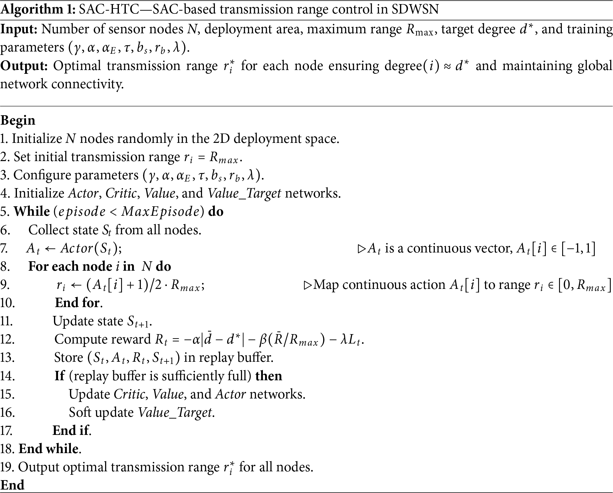
Algorithm 1 presents the pseudocode of the proposed SAC-HTC algorithm, which optimizes sensor-node transmission power to maintain the node degree near the target while preserving global connectivity; after initializing deployment parameters and DRL settings, nodes are distributed, assigned initial power, and iteratively report local states including coordinates, degree from Hello packets, power level, and neighbor lists to the Controller, which aggregates these data, verifies connectivity, and updates the global network state. Based on this, the Actor network generates a continuous action value for adjusting the transmission power of each node. This action, typically a scalar value (e.g., in the range [−1, 1]), is then mapped to a specific transmission power level in the valid operational range [0, Rmax], and the corresponding commands are sent to the nodes. Exploration noise is added during training, and nodes update power levels, recalculate degrees, and send back new states for reward evaluation, which considers degree deviation, energy efficiency, and connectivity penalties. All interactions are stored in a replay buffer for stable learning, while the SAC model is refined through mini-batch sampling, soft updates to the Value target network, dual-Critic Q-value estimation, and entropy-regularized updates to the Value and Actor networks. Once convergence is achieved, the learned policy is applied to maintain the desired average node degree, reduce energy consumption, and preserve connectivity, demonstrating SAC-HTC’s effectiveness in centralized WSNs resource management under the SDWSN framework.

4  Simulation Results and Discussion

4.1 Simulation Scenario

All SAC-HTC experiments were implemented in MATLAB R2024 using the Deep Learning Toolbox™ for constructing and training neural networks. Simulations were executed on a standard workstation (Intel Core i7, 64 GB RAM) without GPU acceleration. Owing to the compact network architecture (<1 MB for N=50–100), all computational operations, including training, were efficiently executed on the CPU.

In simulations with networks of 50 to 100 sensor nodes, SAC-HTC maintains a compact model and low computational cost, making it suitable for medium-scale WSNs. The neural network architecture includes three hidden layers with 64 units each, comprising five sub-networks (one Actor, two Critics, and two Value networks) with approximately 84,000 parameters, where the Actor receives ∼100 input features and outputs a 50-dimensional continuous action vector. The Replay Buffer of 5000 samples accounts for most of the memory usage, keeping the total memory footprint below 11 MB. Training cost primarily arises from backpropagation on 1024-sample batches, while inference requires only a single forward pass of ∼36,000 FLOPs (Floating Point Operations), enabling stable and real-time operation even for networks with up to 100 nodes.

Rmax (maximum transmission range) is measured in meters (m) and fixed at 250 m as described in Section 4.1. Path loss is consistently expressed in decibels (dB). The Energy Efficiency Ratio (EER) is a unitless metric defined in Section 4.2 as

EERi=(riRmax)2(4)

since both ri and Rmax share the same unit (meters), the ratio is dimensionless and presented in percentage form (%) for ease of interpretation.

The reward weight parameters (λ,α,β) were determined through parameter search to impose a clear priority hierarchy. Connectivity receives the highest weight (λ=0.6) to strictly penalize disconnections (Lt=1). Degree optimization follows with α=0.3, allowing the agent to adjust the network toward the desired average degree once connectivity is preserved. Energy consumption has the lowest weight (β=0.1), encouraging the reduction of average transmission range only after higher-priority objectives are satisfied. Experimental results confirm this hierarchy: Set 1 (λ=0.6,α=0.3,β=0.1) yields stable convergence; Set 2 (λ=0.3,α=0.6,β=0.1) is unstable due to excessive emphasis on degree; and Set 3 (λ=0.1,α=0.3,β=0.6) fails completely as the agent prioritizes minimizing transmission range, leading to disconnections.

The experiments are conducted within a two-dimensional area of 1000 × 1000 m2, where sensor nodes are randomly distributed across the entire region, following the deployment approach in [8]. Each node is capable of adjusting its transmission range from a minimum value up to a maximum limit of 250 m. Based on the network connectivity maintenance criteria outlined in previous studies [2,8], the target node degree is set to 4 as the benchmark for evaluating connectivity performance. The SDWSN is simulated with the number of nodes varying from 50 to 90, and each scenario is repeated 10 times to ensure reliability and reproducibility of the results. For the SAC-HTC algorithm, the training process is executed over 100 epochs to achieve a network state where the node degree converges toward the desired value. Detailed simulation parameters are presented in Table 1.

The study applies the Free-Space Path loss (FSPL) model with a fixed Path loss exponent n=2 at an operating frequency f=2.4 GHz. The propagation environment is assumed to be ideal (no obstacles, reflections, or shadowing effects) with unity antenna gain. The Path loss is calculated based on the distance d and the speed of light c using the formula:

Path loss (dB)=10log10⁡((4πfdc)2)(5)

where d is the distance between nodes in meters.

4.2 Simulation Results

Fig. 1 compares the ability of MaxPower, LTRT, DQPLET, and SAC-HTC to maintain an average node degree near the target value of 4 as the network size increases from 50 to 90 nodes. The results show clear differences in accuracy and stability. MaxPower deviates the most, with the average node degree ranging widely from 8.32 to 14.96 two to nearly four times above the target and displaying strong sensitivity to network scale. LTRT is more stable but consistently maintains values between 7.04 and 7.91, almost double the desired degree. In contrast, DQPLET and SAC-HTC show high precision and stability. DQPLET keeps the average node degree between 4.32 and 4.35, with a small and consistent relative error of about 8%–8.75%. SAC-HTC achieves the best performance, maintaining values between 4.27 and 4.30, corresponding to the smallest deviation (0.27–0.30) and the lowest relative error of roughly 6.75%–7.5%. Both methods exhibit strong convergence, but SAC-HTC converges closest to the target and shows the narrowest variation interval (0.03), indicating higher robustness.

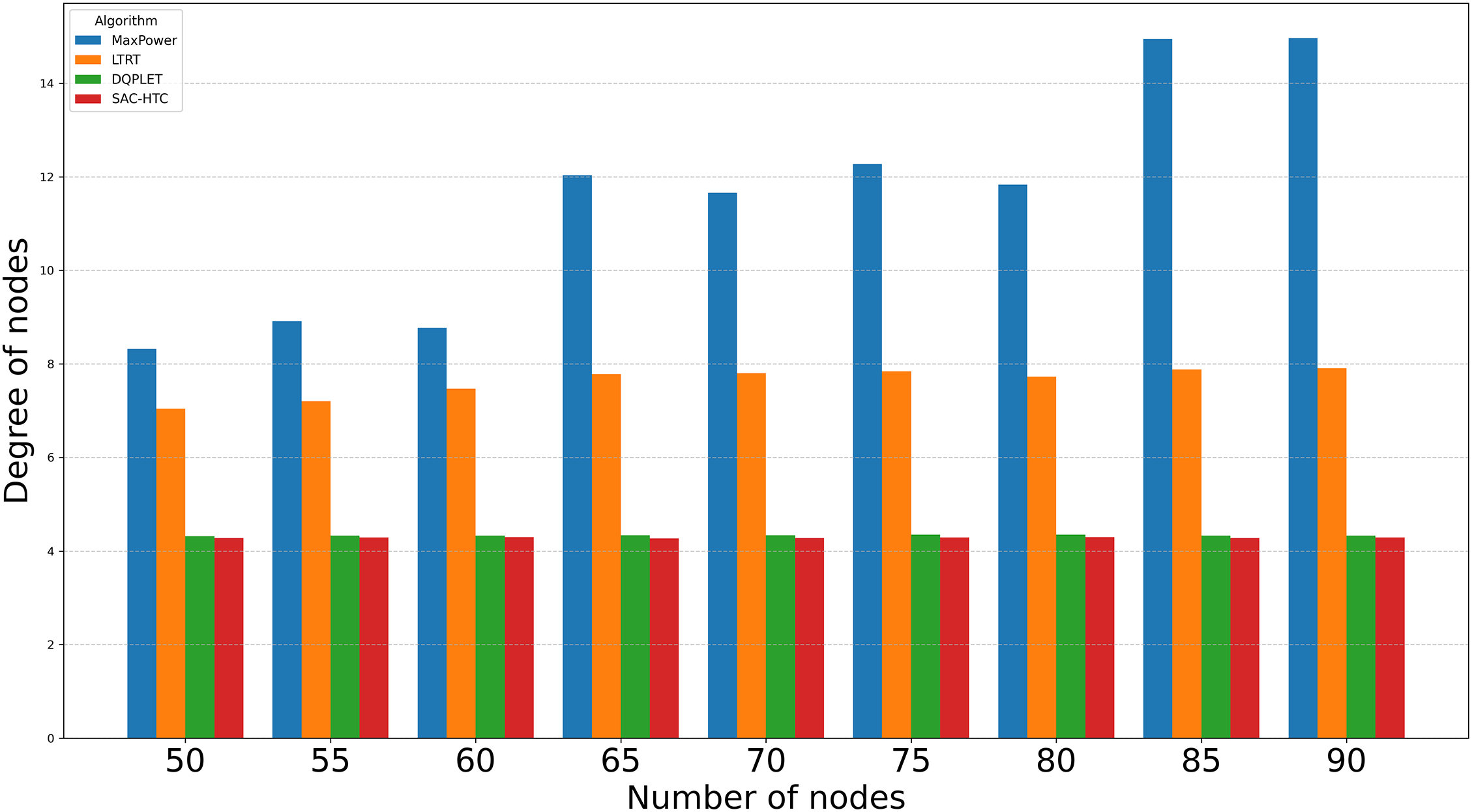
Figure 1: Average node degree vs. the nunber of nodes

A detailed analysis of the Fig. 2 data reveals that both SAC-HTC and DQPLET converge toward the desired node degree of 4; however, SAC-HTC demonstrates significantly higher stability and uniformity. Specifically, the average node degree achieved by DQPLET is approximately 4.34 with a standard deviation of 0.014, while SAC-HTC attains a slightly lower mean value of about 4.285 but with a smaller deviation of 0.009, indicating a more consistent distribution of node degrees and reduced fluctuation across training iterations. In terms of degree distribution, DQPLET exhibits three out of nine samples exceeding the target (above 4.3), one below 4.3, and the remainder concentrated between 4.33 and 4.35, suggesting that several nodes still maintain excessive connectivity, leading to inefficient energy utilization. Conversely, SAC-HTC records only two instances below 4.28 and one above 4.30, meaning that most nodes remain tightly clustered around the target value, effectively balancing connectivity and energy efficiency. Regarding convergence behavior, the SAC-HTC curve exhibits narrow oscillations within the range of 4.27–4.30, whereas DQPLET fluctuates more broadly between 4.32 and 4.35, confirming that SAC-HTC reaches a stable equilibrium more rapidly and maintains steadier performance. These observations demonstrate that SAC-HTC not only achieves node-degree convergence closer to the intended value but also better regulates deviations among nodes, minimizing both under-connected and over-connected cases, thereby optimizing network structure and energy consumption. Overall, SAC-HTC consistently maintains an average node degree near the target with smaller variance and a more balanced distribution, affirming its superiority over DQPLET in ensuring network stability, reducing power expenditure, and enhancing the structural consistency of WSNs.

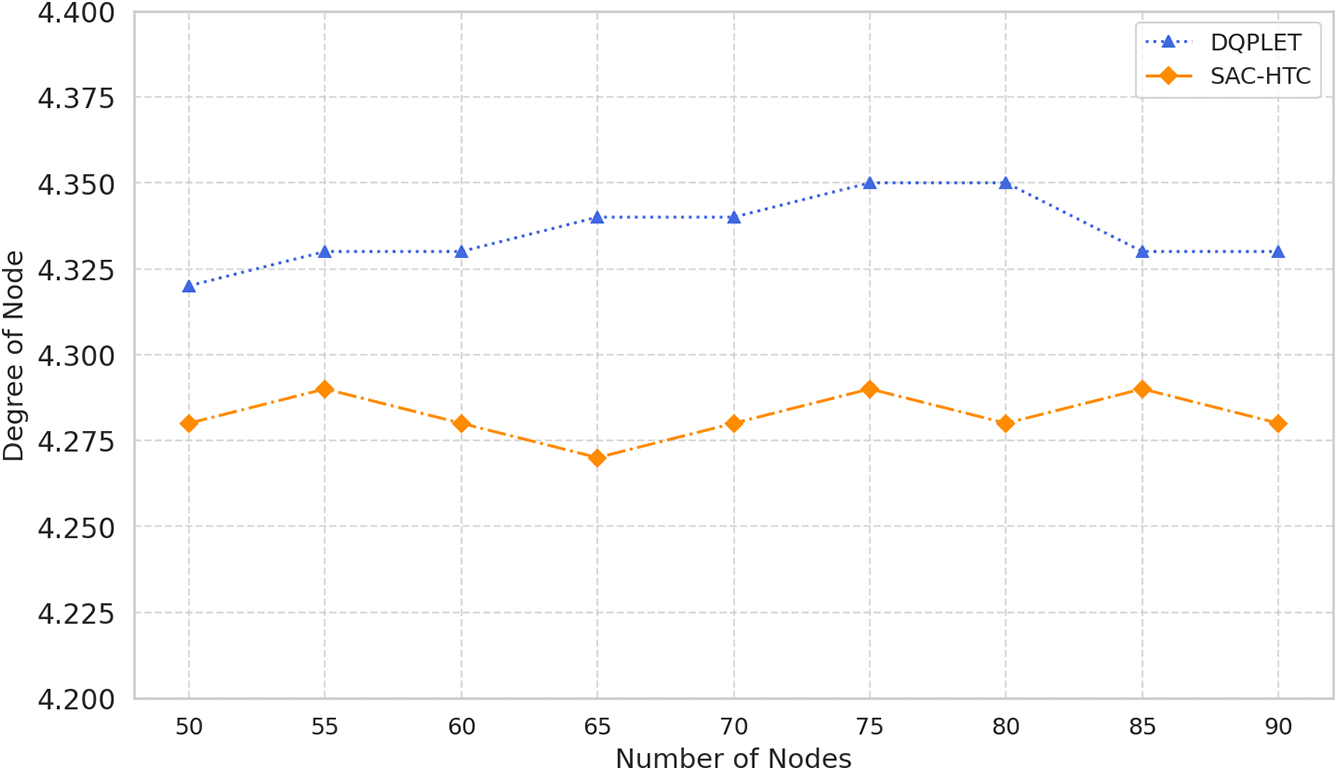
Figure 2: Compare the average node degree of DQPLET and SAC-HTC algorithms

To further clarify the advantages of SAC-HTC over DQPLET in large-scale environments, we conducted experiments with a network size of N = 200 nodes (Fig. 3). The quartile analysis of node degree indicators for the two algorithms reveals a clear distinction in terms of convergence and stability around the target node degree of 4. Specifically, for the DQPLET algorithm, the quartile values are first quartile (Q1) = 4.0, second quartile (Q2) = 5.0, and third quartile (Q3) = 6.0, with an interquartile range (IQR) of 2.0 and an average value of 4.91, indicating a right-skewed distribution where most nodes maintain higher-than-necessary connectivity levels. In contrast, SAC-HTC achieves Q1 = 3.0, Q2 = 4.0, and Q3 = 5.0 with the same IQR = 2.0 but a lower mean value of 4.27, which is much closer to the desired degree. This reflects SAC-HTC’s ability to perform precise and balanced adjustments, with 50% of the nodes having degrees within the range [3,5] a narrower and more concentrated distribution compared to the [4,6] range observed in DQPLET. These results demonstrate that SAC-HTC not only maintains a stable network structure but also minimizes redundant connections, thereby improving energy efficiency and ensuring more optimal communication performance. Overall, across all statistical indicators, SAC-HTC exhibits superior precision, convergence behavior, and adaptability in transmission range control compared to DQPLET.

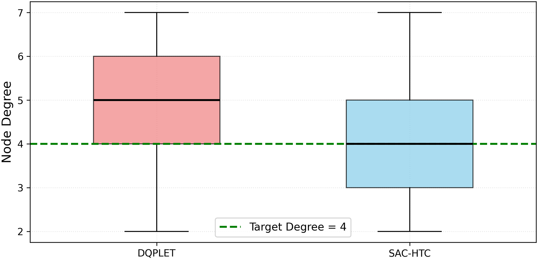
Figure 3: Compare the node degree distributions of DQPLET and SAC-HTC algorithms in case of 200 nodes

Based on the simulation data with 300 nodes, over 120 training episodes, and thousands of iterative steps per episode, the results reveal a significant difference in the convergence capability between the DQPLET and SAC-HTC algorithms in adjusting the node degree toward the desired value of 4 (Fig. 4). In the initial stage, both algorithms exhibit relatively high average node degrees (≈8.24); however, the decreasing trajectory of SAC-HTC is considerably faster than that of DQPLET. Specifically, within the first 20 episodes, SAC-HTC rapidly reduces the average degree from 8.24 to approximately 4.6, approaching the target value and reaching a stable state around 4.32 from Episode 22 onward. In contrast, DQPLET decreases from 8.24 to only about 6.5 after more than 120 episodes, indicating a slower convergence rate and weaker adaptability. The average reduction rate of SAC-HTC during the early phase reaches approximately 0.18 degrees per episode nearly ten times faster than DQPLET (∼0.018 degrees per episode). After reaching the convergence region, SAC-HTC maintains high stability with minor fluctuations (±0.04), whereas DQPLET continues to oscillate around 6.4–6.5, suggesting entrapment in a local optimum and insufficient policy optimization. These findings confirm that SAC-HTC achieves significantly faster, more stable, and more robust convergence compared to DQPLET, enabling the sensor network to quickly reach an optimal topology configuration with an average node degree close to the desired target, while DQPLET remains slower and less efficient in large-scale topology control. The SAC-HTC algorithm, an Actor–Critic method, incurs higher computational cost per training step compared to traditional Q-learning algorithms such as Deep Q-Network (DQN). This increase is an intentional trade-off to achieve stability, high sample efficiency, and the ability to handle continuous action spaces. Unlike DQN, which updates a single Q-network and a Target Q-network, SAC-HTC updates five neural networks: one Actor, two Critics, one Value, and one Target Value, with backpropagation performed on the four main networks, resulting in a per-step computational cost approximately 3–4 times higher. However, in our wireless sensor network scenarios, the dominant computational burden originates not from the learning algorithm itself but from the environment. At each interaction step, the SDN controller must reconstruct the global connectivity graph and check network connectivity, with complexity 𝒪(V+E) or 𝒪(N2) in the worst case, which applies regardless of whether the learning algorithm is SAC or Q-learning.

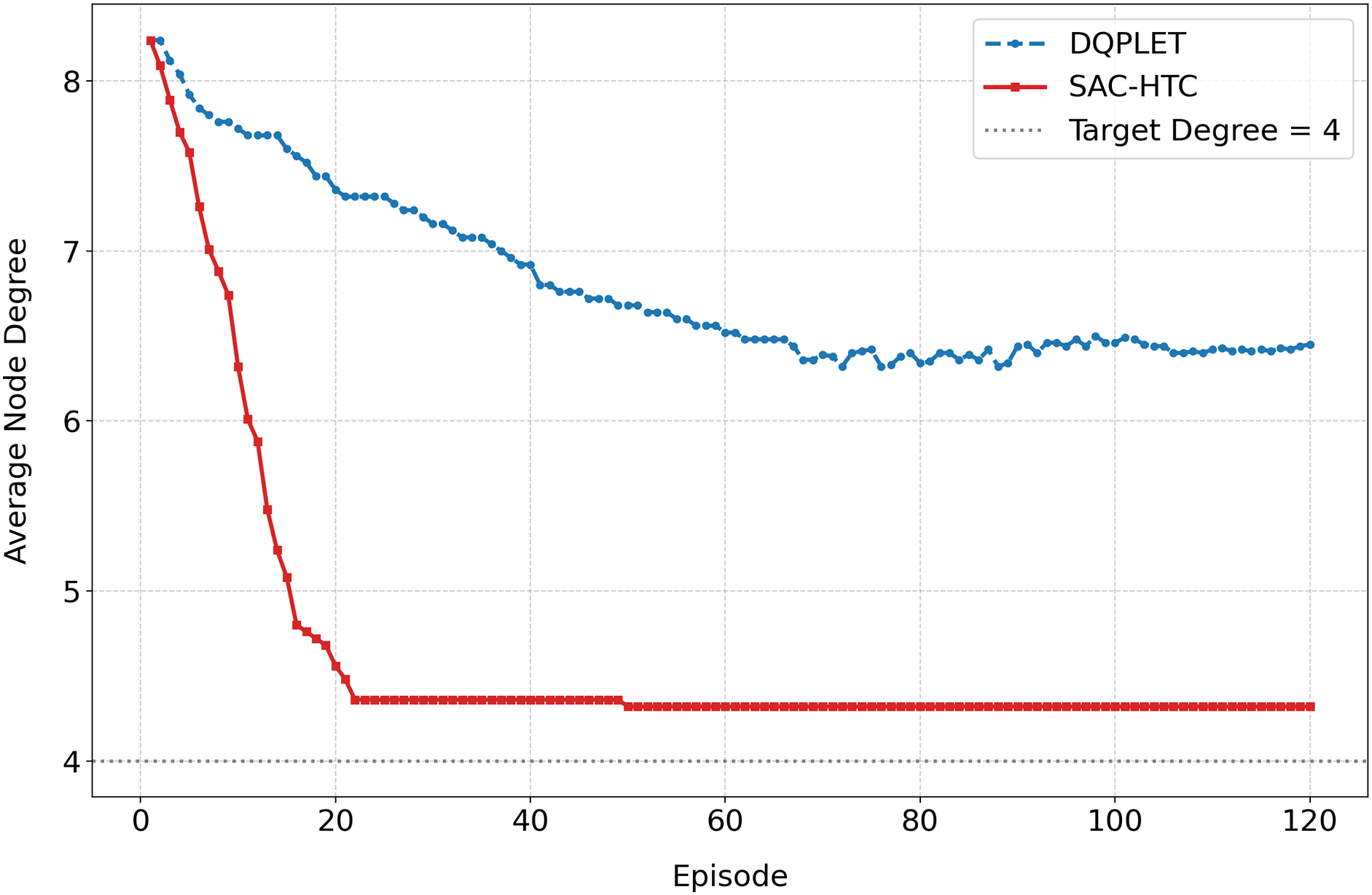
Figure 4: Average node degree vs. training episodes in case of 300 nodes

The EER results in Fig. 5 further highlight the performance differences among the four methods. SAC-HTC achieves the lowest average EER at 38.995%, indicating more effective control of transmission range and closer convergence of the average node degree to the target value. Its distribution is compact, ranging from 28.92% to 48.88%, with most samples clustered within 36%–45%, reflecting stable behavior and a relatively small standard deviation across trials. MaxPower, by contrast, consistently yields an EER of 100%, confirming the absence of power control and severe energy inefficiency. LTRT shows a higher average EER of 68.483% and a wide spread between 57.09% and 79.46%, indicating weak regulation and large variability. DQPLET performs closer to SAC-HTC, with an average of 40.011% and a concentration in the 39%–49% interval, but still presents slightly higher values and broader variation, reflecting less precise degree control. Overall, the narrow box of SAC-HTC demonstrates stronger convergence, lower dispersion, and better energy efficiency, making it the most consistent and accurate method among the evaluated approaches.

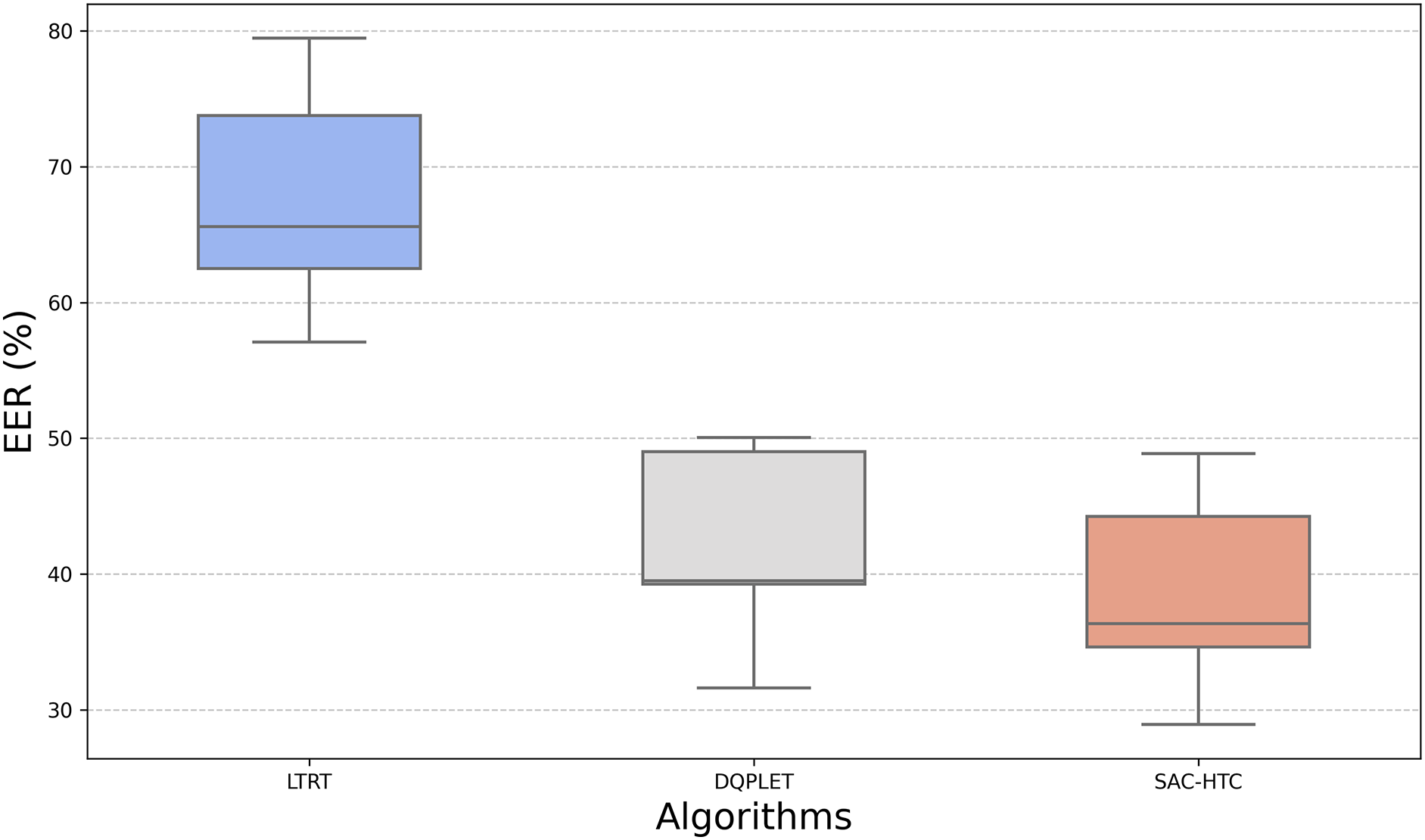
Figure 5: Compare the EER distributions of LTRT, DQPLET and SAC-HTC algorithms

The EER behavior under varying network sizes, illustrated in Fig. 6, reinforces the superiority of SAC-HTC. Across node counts from 50 to 90, SAC-HTC consistently maintains the lowest and most stable EER, ranging from 28.92% to 48.88%. This narrow band indicates strong convergence, small standard deviation, and effective control of transmission range while keeping the average node degree close to the target. Its radar curve remains compact and centered, reflecting minimal deviation and high energy efficiency. MaxPower, by contrast, remains fixed at 100% regardless of network size, confirming its inability to adapt and its complete lack of energy savings. LTRT exhibits high variability, with EER values between 57.09% and 79.46%, demonstrating limited adjustment capability and frequent degree overshooting. DQPLET performs better than LTRT and MaxPower, with values from 31.62% to 50.05%, but still shows higher average EER and weaker convergence than SAC-HTC.

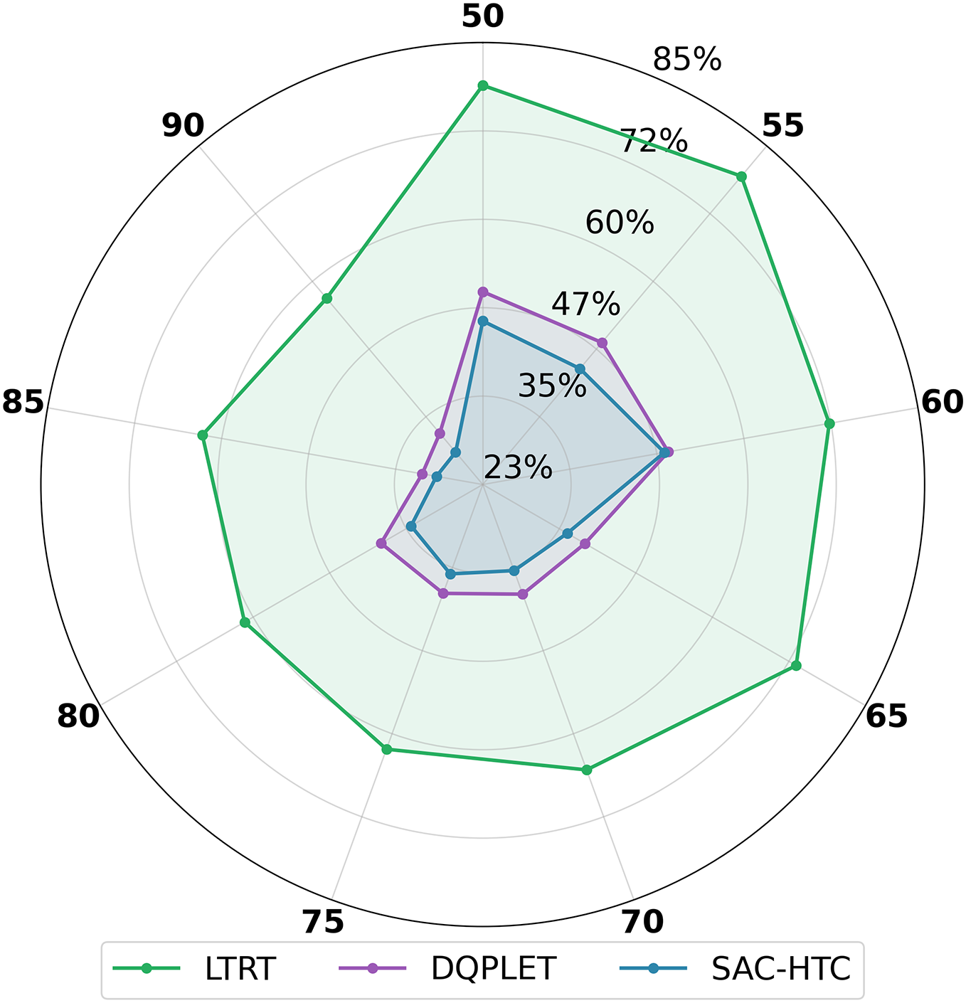
Figure 6: Compare the EER distributions of LTRT, DQPLET and SAC-HTC algorithms using radar chart

The evaluation of the EER across varying network scales is detailed in the line chart shown in Fig. 7. SAC-HTC consistently demonstrates superior energy management, exhibiting a stable and continuous decline in EER from an initial 45.94% down to 28.92% as the network size increases. This trend confirms the algorithm’s effective control over transmission range, allowing the network to achieve and maintain optimal efficiency near the theoretical minimum. In direct contrast, the MaxPower baseline remains static at 100% EER across all scales, confirming continuous operation at maximum power and affirming its inherent energy inefficiency. Among the compared learning methods, DQPLET performed better than LTRT, with its EER decreasing from 50.05% to 32.38%. However, DQPLET consistently operates at a higher energy cost than SAC-HTC. LTRT showed limited optimization capability, maintaining significantly high EER values ranging from 79.00% down to 57.09%. The low magnitude and stability of the SAC-HTC curve validate that its continuous action space and entropy regularization mechanism effectively minimize redundant communication power settings, leading to the most reliable and optimal energy savings for scalable SDWSN.

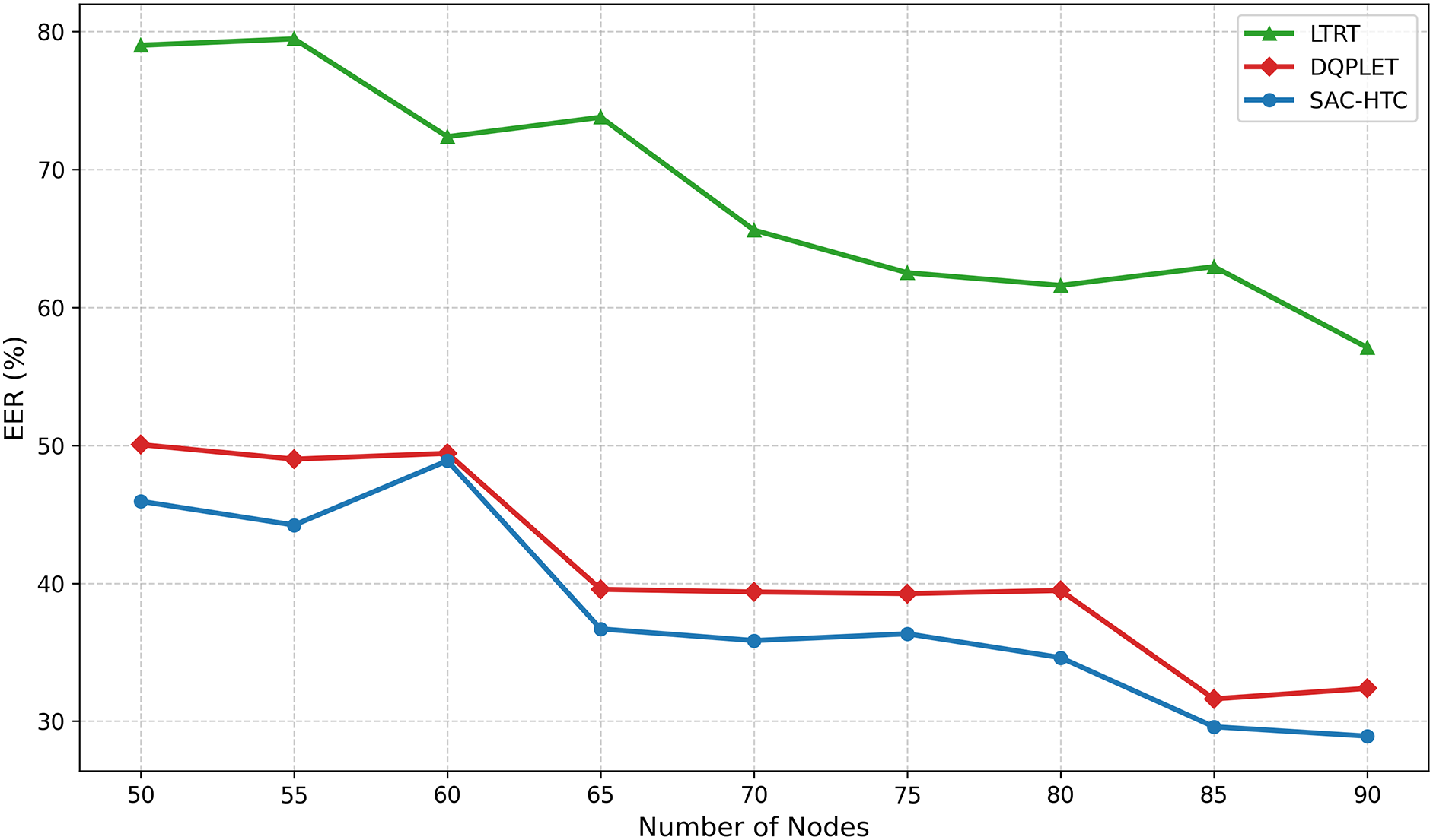
Figure 7: EER vs. the number of nodes

To confirm the advantages of SAC-HTC over DQPLET in terms of the Path loss index (Fig. 8), we conducted experiments on a network with N = 200 sensor nodes. The quartile analysis of the Path loss index for the two algorithms, SAC-HTC and DQPLET, reveals a significant difference in stability and communication efficiency within the wireless sensor network. Specifically, the median (Q2) value of SAC-HTC is 83.5 dB, which is notably lower than 84.8 dB for DQPLET, indicating a better ability to maintain lower and more stable signal attenuation. The Q1 and Q3 of SAC-HTC are 82.8 and 84.0 dB, respectively, while those of DQPLET are 83.8 and 85.2 dB, demonstrating that SAC-HTC exhibits a narrower and more concentrated central distribution. The IQR of SAC-HTC is 1.2, smaller than 1.4 for DQPLET, reflecting less data dispersion and greater overall network stability. Furthermore, the range of SAC-HTC varies from 81.2 to 84.4 dB, whereas DQPLET spans from 82.3 to 85.5 dB, showing that SAC-HTC achieves better consistency in signal attenuation among nodes. Overall, the quartile-based indicators confirm that SAC-HTC not only reduces the average Path loss but also maintains higher communication stability, thereby enhancing energy efficiency and reliability across the wireless sensor network.

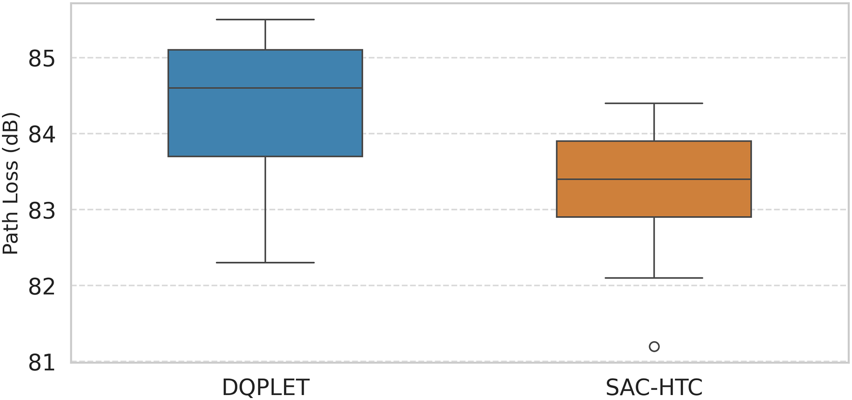
Figure 8: Compare the path loss of SAC-HTC and DQPLET algorithms in case of 200 nodes

Memory usage consists of the model and the replay buffer. The SAC-HTC model employs five neural networks (one Actor, two Critics, and two Value networks), each with three hidden layers of 64 units, totaling approximately 18,000–28,000 parameters, while the replay buffer holds 5000 samples, scaling linearly with the number of nodes N; for N=50 the total memory is ∼10.7 MB, and for N=100∼21 MB. Computational cost includes inference (∼18,000–28,000 parameters per Actor forward pass, taking microseconds on CPU), reward calculation (graph construction and connectivity check, 𝒪(N2), a few milliseconds for N=100), and training (backpropagation through all networks, ∼84,000–126,000 parameters, taking hundreds of milliseconds to a few seconds per batch). SAC’s off-policy nature ensures high sample efficiency, allowing stable convergence after a few thousand environment interaction steps, even when each step involves updating transmission powers, collecting network states, and sending feedback in practical SDN environments.

This Fig. 9 illustrates the adaptation process of the DQPLET and SAC-HTC algorithms to the average node degree when the network experiences failures and subsequent recovery. In the initial stage (Episode <250), when 10% of the nodes are abruptly deactivated, the network’s average degree drops sharply because the failed nodes have zero degree and their neighboring nodes lose links, causing the network to fall into a state of global disconnection, with the average degree reduced to approximately 3.1–3.5 for DQPLET and 2.8–3.3 for SAC-HTC. From Episode 250 to 500, the failed nodes are restored and the allowable communication range is expanded back to the maximum value of 250 m, leading to an increase in the number of links among nodes and a rapid recovery of the network’s average degree. The period from Episode 500 to 700 marks the convergence process, during which DQPLET gradually decreases from 8.3 to around 5.5 at a rate of 0.014 degree per episode, while SAC-HTC decreases faster from 7.4 to 4.6 within approximately 100 episodes at a rate of 0.028 degree per episode. This behavior indicates that SAC-HTC has a significantly shorter settling time of about 150 episodes, compared to DQPLET, which requires 250–300 episodes to reach a steady state. In the steady-state phase (Episode >700), DQPLET fluctuates around 5.5±0.05, whereas SAC-HTC maintains a level close to 4.6±0.03, which is very close to the desired degree (=4). The steady-state fluctuation of SAC-HTC (standard deviation ≈0.03) is nearly 50% lower than that of DQPLET (≈0.06), demonstrating higher stability and a better ability to maintain equilibrium. These results confirm that SAC-HTC exhibits superior adaptability and faster convergence when the network is subjected to node failures and recovery processes, particularly under conditions of abrupt topology changes.

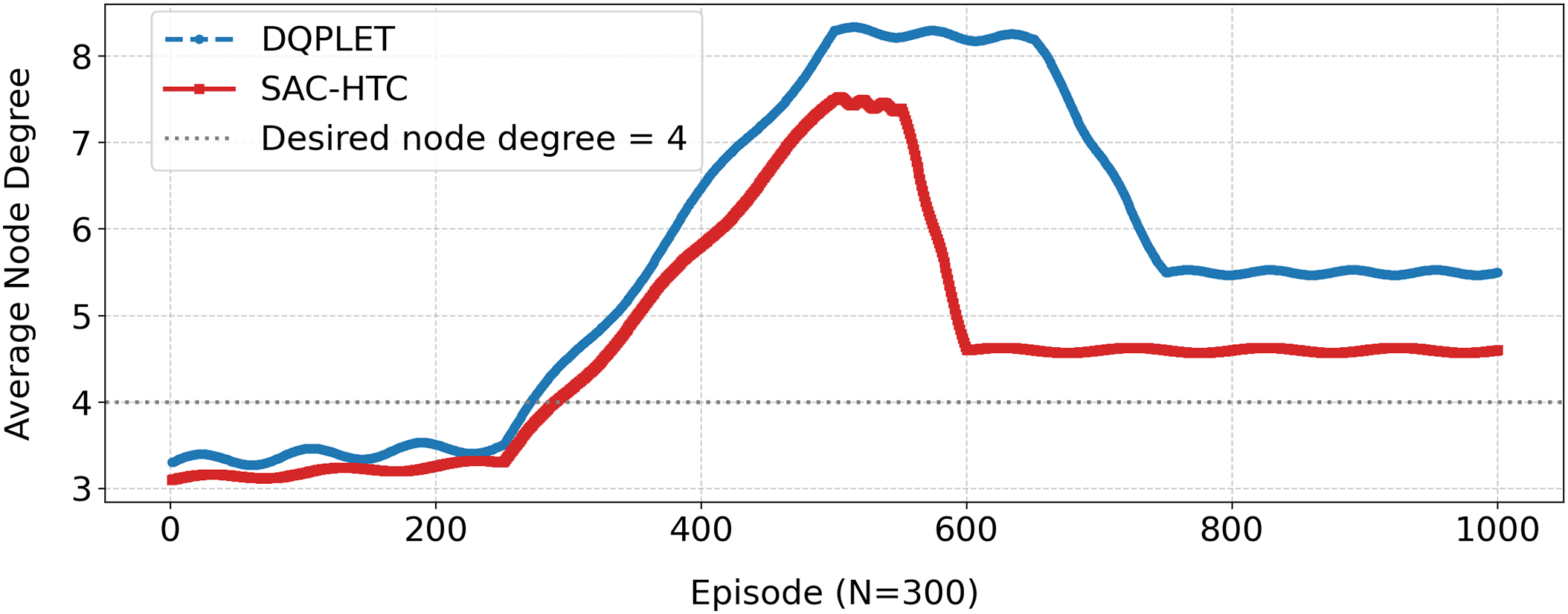
Figure 9: Node degree convergence of DQPLET and SAC-HTC

The dynamic topology control capability of SAC-HTC, managed by an SDN controller, has significant potential for practical applications. In dense urban IoT deployments, such as smart blocks with thousands of sensors for street lighting, parking, traffic monitoring, or pollution tracking, SAC-HTC can minimize interference and save energy by adjusting transmission power to maintain an average node degree d∗=4 while reducing range R, thus extending sensor lifetime. The algorithm also supports self-healing: when node failures fragment the network, SAC-HTC quickly adapts transmission powers of neighboring nodes to restore global connectivity. In UAV-assisted WSNs, SAC-HTC enables real-time topology control, allowing the controller to compute near-optimal transmission powers as UAV positions change, maintaining connectivity while minimizing energy consumption. These scenarios demonstrate the practical relevance and adaptability of SAC-HTC in dynamic, resource-constrained networks.

5  Conclusion

This study introduced and evaluated the SAC-HTC algorithm within the SDWSN framework as an intelligent network topology control mechanism based on DRL, aiming to simultaneously optimize node degree stability, energy efficiency, and communication reliability. Empirical analysis demonstrated that SAC-HTC maintains a stable average node degree around the target value of 4 with minimal deviation, indicating precise control capability and adaptive flexibility. Compared to DQPLET, LTRT, and MaxPower, SAC-HTC achieved significantly superior performance by maintaining a uniform node degree distribution, minimizing outliers, and balancing connectivity with energy efficiency. Regarding energy efficiency, SAC-HTC consistently achieved the lowest EER across all scenarios, averaging around 39% compared to 68% for LTRT and 100% for MaxPower, while the narrow EER range from 29% to 49% reflected stable energy control. Furthermore, the path loss results reinforced SAC-HTC’s effectiveness, with an average value of approximately 81.3 dB, indicating efficient signal transmission. Overall, SAC-HTC achieves an optimal balance between connectivity, energy efficiency, and signal reliability through an entropy-regularized RL mechanism that enables continuous adaptation, fast convergence, and more effective self-organization than static or heuristic-based approaches.

Based on the obtained results, alongside its advantages, this study also highlights opportunities to address scalability limitations of the current centralized model. Future research will focus on developing distributed or multi-agent RL mechanisms to reduce controller load, enabling better adaptation to large-scale networks with hundreds or thousands of nodes. Additionally, the algorithm can be extended to complex hybrid and dynamic network environments, such as integrated SDWSN-UAVNET (Unmanned Aerial Vehicle Network) architectures, smart city infrastructures, and industrial IoT systems with highly mobile nodes. The integration of transfer learning and hybrid optimization models will also be explored to improve training speed and network resilience. Finally, a crucial next step is deploying the algorithm on real hardware platforms to comprehensively validate simulation accuracy. Therefore, SAC-HTC not only establishes a robust foundation for intelligent and energy-efficient network control but also represents a pioneering framework ready for expansion and application in next-generation WSNs.

Acknowledgement: Not applicable.

Funding Statement: The authors received no specific funding for this study.

Author Contributions: The authors confirm contribution to the paper as follows: Conceptualization, Ho Hai Quan; methodology, Ho Hai Quan and Le Huu Binh; software, Ho Hai Quan; validation, Ho Hai Quan and Nguyen Dinh Hoa Cuong; formal analysis, Le Huu Binh and Le Duc Huy; investigation, Ho Hai Quan and Le Huu Binh; resources, Nguyen Dinh Hoa Cuong and Le Duc Huy; data curation, Ho Hai Quan; writing original draft preparation, Ho Hai Quan; writing, review and editing, Le Huu Binh; visualiza-tion, Le Duc Huy; supervision, Le Huu Binh; project administration, Ho Hai Quan. All authors reviewed and approved the final version of the manuscript.

Availability of Data and Materials: Not applicable.

Ethics Approval: Not applicable.

Conflicts of Interest: The authors declare no conflicts of interest to report regarding the present study.

References

1. Hai HTC, Binh LH, Huy LD. A topology control algorithm taking into account energy and quality of transmission for software-defined wireless sensor network. Int J Comput Netw Commun. 2024;16(2):107–16. doi:10.5121/ijcnc.2024.16207. [Google Scholar] [CrossRef]

2. Miyao K, Nakayama H, Ansari N, Kato N. LTRT: an efficient and reliable topology control algorithm for ad-hoc networks. IEEE Trans Wireless Commun. 2009;8(12):6050–8. doi:10.1109/twc.2009.12.090073. [Google Scholar] [CrossRef]

3. Du Z, Wang S, Wang X, Chen J. Formation-aware UAV network self-organization with game-theoretic distributed topology control. IEEE Trans Cogn Commun Netw. 2025;11(5):3470–85. doi:10.1109/tccn.2025.3530443. [Google Scholar] [CrossRef]

4. Zhao H, Chen H, Li S, Zhan L. Joint optimization of UAV trajectory and number of reflecting elements for UAV-carried IRS-assisted data collection in WSNs under hover priority scheme. IEEE Syst J. 2025;19(3):963–74. doi:10.1109/jsyst.2025.3607118. [Google Scholar] [CrossRef]

5. Binh LH, Duong TVT. A novel and effective method for solving the router nodes placement in wireless mesh networks using reinforcement learning. PLoS One. 2024;19(4):e0301073. doi:10.1371/journal.pone.0301073. [Google Scholar] [PubMed] [CrossRef]

6. Binh LH, Duong TVT, Ngo VM. TFACR: a novel topology control algorithm for improving 5G-based MANET performance by flexibly adjusting the coverage radius. IEEE Access. 2023;11:105734–48. doi:10.1109/access.2023.3318880. [Google Scholar] [CrossRef]

7. Qi W, Shen J, Zhang X, Lan T, Diao R, Liu J, et al. Intelligent topology control of distribution power network for increased clean energy absorption using reinforcement learning. In: Proceedings of the 2025 10th Asia Conference on Power and Electrical Engineering (ACPEE); 2025 Apr 15–19; Beijing, China. p. 240–4. doi:10.1109/acpee64358.2025.11040504. [Google Scholar] [CrossRef]

8. Ho HQ, Le HB, Nguyen DHC. Deep Q-learning-based path loss and energy-efficient topology control for wireless sensor networks. Int J Innov Comput Inf Control. 2025;21(6):1503–22. doi:10.3724/sp.j.1001.2009.03414. [Google Scholar] [CrossRef]

9. Ding Z, Shen L, Chen H, Yan F, Ansari N. Energy-efficient topology control mechanism for IoT-oriented software-defined WSNs. IEEE Internet Things J. 2023;10(15):13138–54. doi:10.1109/jiot.2023.3260802. [Google Scholar] [CrossRef]

10. Younus MU, Khan MK, Bhatti AR. Improving the software-defined wireless sensor networks routing performance using reinforcement learning. IEEE Internet Things J. 2022;9(5):3495–508. doi:10.1109/jiot.2021.3102130. [Google Scholar] [CrossRef]

11. Tyagi V, Singh S, Wu H, Gill SS. Load balancing in SDN-enabled WSNs toward 6G IoE: partial cluster migration approach. IEEE Internet Things J. 2024;11(18):29557–68. doi:10.1109/jiot.2024.3402266. [Google Scholar] [CrossRef]

12. Yoo T, Lee S, Yoo K, Kim H. Reinforcement learning based topology control for UAV networks. Sensors. 2023;23(2):921. doi:10.3390/s23020921. [Google Scholar] [PubMed] [CrossRef]

13. Li J, Yi P, Duan T, Wang Y, Zhang Z, Yu J, et al. Centroid-guided target-driven topology control method for UAV ad-hoc networks based on tiny deep reinforcement learning algorithm. IEEE Internet Things J. 2024;11(12):21083–91. doi:10.1109/jiot.2024.3376647. [Google Scholar] [CrossRef]

14. Zhao Z, Liu C, Guang X, Li K. A transmission-reliable topology control framework based on deep reinforcement learning for UWSNs. IEEE Internet Things J. 2023;10(15):13317–32. doi:10.1109/jiot.2023.3262690. [Google Scholar] [CrossRef]

15. Asmat H, Ud Din I, Almogren A, Khan MY. Digital twin with soft actor-critic reinforcement learning for transitioning from industry 4.0 to 5.0. IEEE Access. 2025;13:40577–93. doi:10.1109/access.2025.3546085. [Google Scholar] [CrossRef]

16. Siddiqua A, Liu S, Siddika Nipu A, Harris A, Liu Y. Co-evolving multi-agent transfer reinforcement learning via scenario independent representation. IEEE Access. 2024;12:99439–51. doi:10.1109/access.2024.3430037. [Google Scholar] [CrossRef]

17. Lautenbacher T, Rajaei A, Barbieri D, Viebahn J, Cremer JL. Multi-objective reinforcement learning for power grid topology control. In: Proceedings of the 2025 IEEE Kiel PowerTech; 2025 Jun 29–Jul 3; Kiel, Germany. p. 1–7. doi:10.1109/powertech59965.2025.11180236. [Google Scholar] [CrossRef]

18. Anshad AS, Geetha MN, Rajyalaxmi S, Ganesha M, Kaliappan S, Suganthi D. A blockchain-enabled secure and energy-efficient routing protocol for wireless sensor networks in environmental monitoring using RL-DDPGA. In: Proceedings of the 2025 1st International Conference on Radio Frequency Communication and Networks (RFCoN); 2025 Jun 19–20; Thanjavur, India. p. 1–6. doi:10.1109/rfcon62306.2025.11085190. [Google Scholar] [CrossRef]

19. Yang J, Li W, Li C, Zhang L, Liu L. An energy-efficient and transmission-efficient adaptive routing algorithm using deep reinforcement learning for wireless sensor networks. IEEE Internet Things J. 2025;12(23):50414–26. doi:10.1109/jiot.2025.3609624. [Google Scholar] [CrossRef]

20. Rose B, Nivithaa AN, Parthiban V, Sedhupathi RB, Kannan AT. Intelligent energy-efficient routing in wireless. In: Proceedings of the 2025 3rd International Conference on Artificial Intelligence and Machine Learning Applications; 2025 Apr 29–30; Namakkal, India. p. 1–6. doi:10.1109/aimla63829.2025.11040373. [Google Scholar] [CrossRef]

21. Yadav DK, Nagappan B. Energy communication conservation of methods for 6G and 5G for future performance and training. In: Proceedings of the 2025 1st International Conference on Advances in Computer Science, Electrical, Electronics, and Communication Technologies (CE2CT); 2025 Feb 21–22; Bhimtal, India. p. 503–8. doi:10.1109/ce2ct64011.2025.10939215. [Google Scholar] [CrossRef]

22. Anshad AS, Babavali SF, Cephas I, Ramanan SV, Lakshmi Priya G, Mishra S. An intelligent hybrid quantum-deep reinforcement framework for energy-efficient routing in wireless sensor networks. In: Proceedings of the 2025 6th International Conference for Emerging Technology (INCET); 2025 May 23–25; Belgaum, India. p. 1–6. doi:10.1109/incet64471.2025.11140843. [Google Scholar] [CrossRef]

23. Priyadarshi R, Teja PR, Vishwakarma AK, Ranjan R. Effective node deployment in wireless sensor networks using reinforcement learning. In: Proceedings of the 2025 IEEE 14th International Conference on Communication Systems and Network Technologies (CSNT); 2025 Mar 7–9; Bhopal, India. p. 1113–8. doi:10.1109/csnt64827.2025.10968953. [Google Scholar] [CrossRef]

24. Huang Z, Wang F, Su C, Wang Y, Liu H. Reinforcement learning-driven hunter-prey algorithm applied to 3D underwater sensor network coverage optimization. IEEE Access. 2025;13:78161–81. doi:10.1109/access.2025.3565953. [Google Scholar] [CrossRef]

25. Gurav S, Rangamani TP, Muthusundar SK, Charumathi AC, Nidhya MS, Maram B. Machine learning models for energy consumption sensors in wireless sensor networks. In: Proceedings of the 2025 International Conference on Modern Sustainable Systems (CMSS); 2025 Aug 12–14; Shah Alam, Malaysia. p. 172–7. doi:10.1109/cmss66566.2025.11182560. [Google Scholar] [CrossRef]

26. Alsaeedi M, Mohamad MM, Al-Roubaiey A. SSDWSN: a scalable software-defined wireless sensor networks. IEEE Access. 2024;12:21787–806. doi:10.1109/access.2024.3362353. [Google Scholar] [CrossRef]

27. Sheela V, Rathiga P. Reinforcement learning-based greedy multi-hop routing protocol using for optimizing WSN. In: Proceedings of the 2025 8th International Conference on Computing Methodologies and Communication (ICCMC); 2025 Jul 23–25; Erode, India. p. 6–14. doi:10.1109/iccmc65190.2025.11140740. [Google Scholar] [CrossRef]

28. Packiyalakshmi P, Ramathilagam A. HyRA-WSN: a hybrid reinforcement-attention model for intelligent and energy-efficient resource allocation in wireless sensor networks. In: Proceedings of the 2025 3rd International Conference on Self Sustainable Artificial Intelligence Systems (ICSSAS); 2025 Jun 11–13; Erode, India. p. 635–41. doi:10.1109/icssas66150.2025.11080922. [Google Scholar] [CrossRef]

29. Singh BP, Taneja A. Self-adaptive AI framework for QoS optimisation and energy efficiency in wireless sensor networks. In: Proceedings of the 2025 3rd World Conference on Communication & Computing (WCONF); 2025 Jul 25–27; Raipur, India. p. 1–6. doi:10.1109/wconf64849.2025.11233718. [Google Scholar] [CrossRef]

30. Singh BP, Taneja A. AI-driven QoS management in wireless sensor networks: enhancing energy efficiency and network performance. In: Proceedings of the 2025 3rd World Conference on Communication & Computing (WCONF); 2025 Jul 25–27; Raipur, India. p. 1–7. doi:10.1109/wconf64849.2025.11233612. [Google Scholar] [CrossRef]

31. Chen N, Wen R, Ma S, Wang P. Improved PEGASIS routing protocol for wireless sensor networks. In: Proceedings of the IEEE International Applied Engineering and Artificial Intelligence Conference; 2024 Mar 15–17; Chongqing, China. Vol. 7. p. 534–8. doi:10.1109/iaeac59436.2024.10503997. [Google Scholar] [CrossRef]

32. Sudhir ACH, Pattabhi Ram GS, Srinivas Raghava A, Katuri EP. Efficient topology control and depth adjustment technique for connectivity in UWSN. In: Proceedings of the 2024 4th International Conference on Pervasive Computing and Social Networking (ICPCSN); 2024 May 3–4; Salem, India. p. 592–6. doi:10.1109/icpcsn62568.2024.00099. [Google Scholar] [CrossRef]

33. Aleem A, Thumma R. Hybrid energy-efficient clustering with reinforcement learning for IoT-WSNs using knapsack and K-means. IEEE Sens J. 2025;25(15):30047–59. doi:10.1109/jsen.2025.3582381. [Google Scholar] [CrossRef]

34. Schneider R, da Silva Alves CA, Assis L, de Farias CM, Mendonça I, González PH. A hybrid multi-centrality and reinforcement learning approach for sensor allocation in wireless sensor networks. In: Proceedings of the 2025 28th International Conference on Information Fusion (FUSION); 2025 Jul 7–11; Rio de Janeiro, Brazil. p. 1–7. doi:10.23919/fusion65864.2025.11124024. [Google Scholar] [CrossRef]

35. Wei D, Yang E, He Y. Topology control and optimization of self-organized networks for wireless personal communication. In: Proceedings of the 2023 IEEE 6th International Conference on Automation, Electronics and Electrical Engineering (AUTEEE); 2023 Dec 15–17; Shenyang, China. p. 462–7. doi:10.1109/auteee60196.2023.10407620. [Google Scholar] [CrossRef]

36. Xue Y, Wang Z, Liu L, Fang C, Sun Y, Chen H. UAV-assisted control design with stochastic communication delays. In: Proceedings of the 2022 IEEE 8th International Conference on Computer and Communications (ICCC); 2022 Dec 9–12; Chengdu, China. p. 707–10. doi:10.1109/iccc56324.2022.10065686. [Google Scholar] [CrossRef]

37. Kipongo J, Swart TG, Esenogho E. Artificial intelligence-based intrusion detection and prevention in edge-assisted SDWSN with modified honeycomb structure. IEEE Access. 2023;12:3140–75. doi:10.1109/access.2023.3347778. [Google Scholar] [CrossRef]

38. Udayaprasad PK, Shreyas J, Srinidhi NN, Dilip Kumar SM, Dayananda P, Askar SS, et al. Energy efficient optimized routing technique with distributed SDN-AI to large scale I-IoT networks. IEEE Access. 2023;12:2742–59. doi:10.1109/access.2023.3346679. [Google Scholar] [CrossRef]