Graph Representation Consistency Enhancement via Graph Transformer for Fault Diagnosis of Complex Industrial Systems

1  Introduction

With the rapid development of modern industry and manufacturing, the scale of industrial systems has expanded, their structures have become increasingly complex, and the operation and maintenance costs have risen sharply. In this context, effectively mitigating system performance degradation, avoiding productivity loss, and preventing potential safety hazards have become critical issues that need to be addressed in the industrial sector [1]. Timely and accurate identification of system operating conditions and fault diagnosis are of great significance for ensuring the safe and stable operation of industrial production and extending the lifespan of equipment [2–4].

Currently, modern industrial systems are typically equipped with large-scale monitoring networks consisting of numerous sensors and measurement devices, generating data with high dimensionality and strong coupling characteristics. Due to the complex interactions between components in industrial systems, local faults often propagate through the process, causing multiple monitoring parameters to go abnormal [5]. This “one cause, multiple effects” fault propagation pattern results in highly nonlinear fault features [6]. Traditional detection methods, which rely on manual experience, are not only inefficient but also struggle to handle increasingly complex industrial scenarios.

The rapid advancement of computer technology and real-time sensor monitoring techniques have provided new technical pathways for automatic industrial fault diagnosis. The vast amount of data collected by sensors provides strong support for fault diagnosis in industrial systems, leading to a growing demand for data analysis. Currently, intelligent fault diagnosis methods can be broadly classified into three categories: model-based methods, knowledge-driven methods, and data-driven methods [7,8]. Model-based diagnostic methods, although they have clear physical significance, heavily rely on precise system modeling. When dealing with complex industrial systems, they face challenges in terms of modeling difficulty and high costs. Knowledge-driven methods, such as expert systems, avoid complex modeling processes and offer good interpretability, but their diagnostic performance is severely limited by the completeness of the expert knowledge base. In contrast, data-driven methods, such as deep learning [9] and transfer learning,can automatically extract fault features from massive monitoring data without requiring prior system knowledge. These methods are efficient in modeling and highly adaptable, offering significant advantages. By utilizing multi-layer nonlinear neural networks for feature learning from raw data, these methods transform the fault diagnosis problem in complex industrial systems into a pattern recognition task for multi-source time-series signals, which has attracted widespread attention in both academia and industry in recent years.

However, most existing data-driven methods focus on analyzing signals from individual sensors and process structured data in Euclidean space, while neglecting the inherent topological structure and dynamic coupling relationships between components in industrial systems [10,11]. This approach struggles to accurately characterize the complex interaction mechanisms found in real-world industrial systems [12]. In fact, graph data is naturally suited for describing systems with topological relationships [13]—mapping each sensor to a graph node and modeling the interactions between components as edges allows the system’s operational state to be represented as a dynamic graph structure [14]. Graph-based algorithms have demonstrated unique advantages in industrial fault diagnosis, with Graph Neural Networks (GNNs) emerging as a research hotspot due to their excellent capability to extract topological features [6,15]. GNNs can effectively capture spatial dependencies between components and construct diagnostic systems by modeling graph data, thereby transforming fault diagnosis into a graph classification task [16,17].

It is worth noting that traditional GNNs still have significant limitations during application: Inconsistency in feature representation between layers during model training can negatively affect diagnostic performance [18]. This issue manifests as inconsistent similarity patterns when graph representations evolve through the network. For example, as shown in Fig. 1, although Graph 1 is more similar to Graph 2 than to Graph 3 at the first layer, the relationship reverses at the second layer. This change in relative similarity indicates that the internal feature hierarchy becomes unstable as depth increases, which is inconsistent with the properties expected of a high-quality feature extractor—one that should maintain feature stability across layers. To address the challenge, this paper proposes a graph Transformer-based fault diagnosis method optimized for consistency. The proposed method provides a new technical approach for fault diagnosis in complex industrial systems. The following sections will detail the methodology, experimental validation, and result analysis. The main contributions of this paper are outlined as follows:

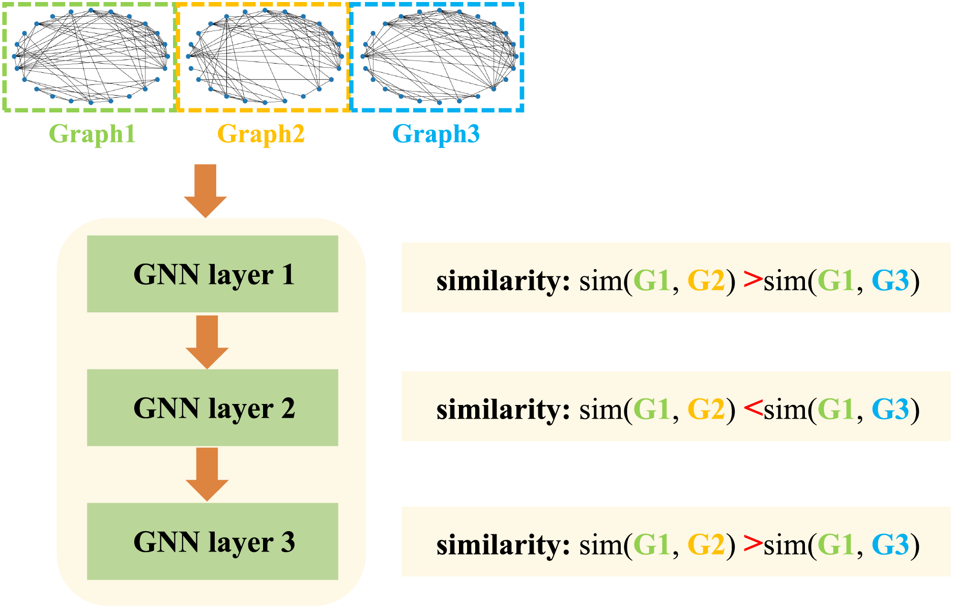
Figure 1: Example of inconsistency in Graph neural networks

1.   Graph-Based Modeling of Multi-Sensor Data: We model multi-sensor data as graph structures, treating each sensor as a node and dynamically constructing edges based on inter-node similarity. A Graph Transformer is then employed to extract graph features through attention mechanisms, enabling adaptive modeling of complex inter-sensor relationships.

2.   Consistency-Constrained Graph Representation Learning: To address the feature inconsistency issue across different layers in graph neural networks (GNNs), we introduce a consistency-guided graph representation learning strategy. By encouraging aligned representations across network layers, the proposed method yields more stable graph representations.

3.   Performance Verification on the TFF Dataset: Experimental results on the TFF dataset demonstrate that our method achieves superior diagnostic performance compared with several existing GNN-based approaches. Ablation studies further verify the effectiveness of the proposed consistency loss.

2  Proposed Method

In this paper, we propose a novel method ConGTransformer to enhance the performance of Graph Neural Networks (GNNs) by enforcing consistency in graph representations across different layers. We use Graph Transformer [19] as the feature extraction backbone, leveraging a consistency loss to ensure the relative similarities of graphs is preserved at each layer of the model. The core innovation in our method is the introduction of consistency loss, which ensures that the relative similarities between graphs remain consistent across layers.

2.1 Overview of Proposed Method

As shown in Fig. 2, we propose a novel method ConGTransformer for fault diagnosis in complex industrial systems, leveraging the strengths of graph-based techniques and deep learning. Initially, sensor measurements are modeled as graph-structured data using the k-nearest neighbors (KNN) algorithm [20,21]. Each sensor node is connected to its k most similar neighbors, forming a graph that represents the relational structure of the sensor data. These graph representations are then passed through multiple Graph Transformer layers, which aggregate neighboring node features using the multi-head self-attention mechanism. Then we use a readout function to aggregate node-level features into graph-level features. After that, the graph-level features are fed into a multilayer perceptron (MLP) for classification, where the final diagnosis is made. To ensure the consistency of graph representations across Graph Transformer layers, a consistency loss is introduced, in addition to the cross-entropy loss. This combined loss function helps preserve the ranking of similarities between graphs across Graph Transformer layers and ensures that the learned representations of the graphs remain stable and consistent, significantly improving fault diagnosis accuracy.

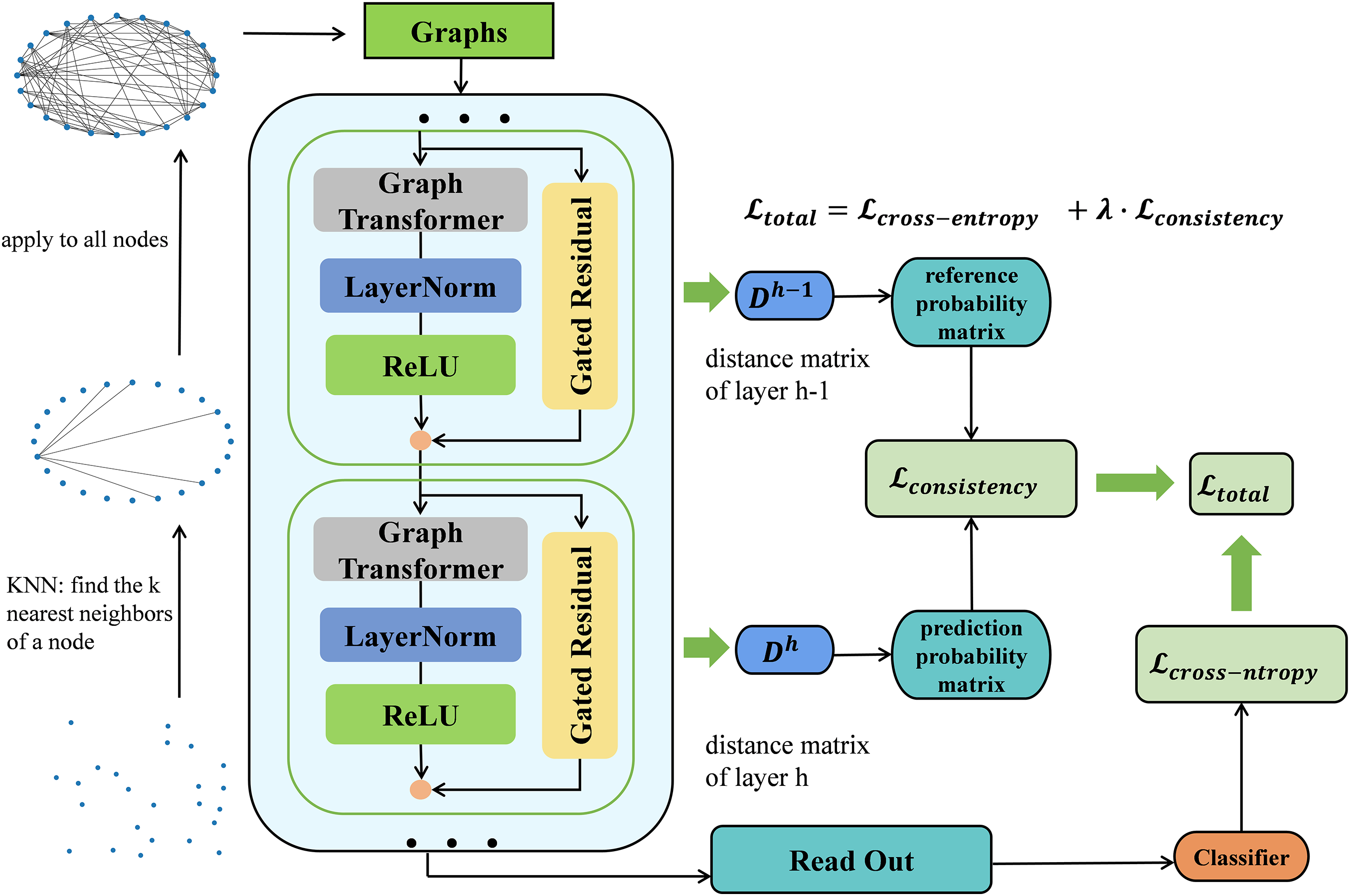
Figure 2: Framework of the proposed fault diagnosis method

2.2 Problem Formulation

Let the industrial system consist of n sensors. For each sensor vi (i=1,2,…,n), the raw time-series signal generated during its operation is a long-span sequence, which is hard to perform real-time fault diagnosis. To address this problem, we use a sliding window to extract stable short-term signal fragments for characterizing the system state around a specific time: given a window size d, the signal fragment of the ith sensor component is a d-dimensional vector xi∈Rd.

Due to the complex interactions among the sensors in the industrial system, we use an undirected input graph G=(V,E) to model the system state, where each vi∈V corresponds to a sensor in the industrial system, the node feature matrix is X=[x1,x2,...,xn]T∈Rn×d.

Then we use edges to represent the interactions between sensors, which are determined by the similarity of node features. For a pair of distinct nodes (vi,vj), the similarity between them is defined as: si,j=11+‖xi−xj‖2. Given a similarity threshold θ, an edge ei,j∈E if and only if si,j>θ. The number of edges connected to node vi is ki=∑j=1,j≠inI(si,j>θ), where I(⋅) denotes the indicator function. The adjacency matrix A∈Rn×n, is defined such that A[i,j]=1 if and only if ei,j∈E, otherwise A[i,j]=0. The task of industrial system fault diagnosis is to train a model f(⋅), which maps the current state G∈𝒢 of the system to a label y∈𝒴.

2.3 Graph Transformer

In this work, we adopt Graph Transformer [19] as the feature extraction backbone. Similar to the standard Transformer, it incorporates graph structure by restricting attention to node neighborhoods, enabling the model to capture meaningful sensor interactions.

Specifically, we use a L-layer Graph Transformer to aggregate node features. Given the input features of the lth layer H(l)=[h1(l),h2(l),...,hn(l)]T∈Rn×d (H(1)=X), We first project the features of the target node i into query vectors qc,i(l)∈RD, and project the features of the source node j into key vectors kc,j(l)∈RD and value vectors vc,j(l)∈RD as follows:

qc,i(l)=Wc,q(l)hi(l)+bc,q(l),(1)

kc,j(l)=Wc,k(l)hj(l)+bc,k(l),(2)

vc,j(l)=Wc,v(l)hj(l)+bc,v(l)(3)

then, we compute multi-head attention weight for each directed edge from source node j to target node i as follows:

αc,ij(l)=⟨qc,i(l),kc,j(l)⟩∑u∈N(i)⟨qc,i(l),kc,u(l)⟩,(4)

where ⟨q,k⟩=exp⁡(qTkD) represents a scaled dot-product attention function with exponential normalization, and D denotes the hidden dimensionality of each attention head. For the cth attention head, the targrt node features hi(l) and the source node features hj(l) are independently projected into query vectors qc,i(l), key vectors kc,j(l) and value vectors vc,j(l) using distinct trainable parameters Wc,q(l)∈RD×d, Wc,k(l)∈RD×d, Wc,v(l)∈RD×d, bc,q(l)∈RD, bc,k(l)∈RD, bc,v(l)∈RD.

Once the graph-based multi-head attention is computed, we perform message aggregation from source node j to target node i. This process is illustrated as follows, where ‖ denotes the concatenation of outputs from all C attention heads.

h^i(l+1)=‖c=1C[∑j∈N(i)αc,ij(l)vc,j(l)].(5)

Then, a gated residual connection is used to prevent our model from oversmoothing as follows:

ri(l)=Wr(l)hi(l)+br(l),(6)

βi(l)=sigmoid(Wg(l)[h^i(l+1);ri(l);h^i(l+1)−ri(l)]),(7)

hi(l+1)=ReLU(LayerNorm((1−βi(l))h^i(l+1)+βi(l)ri(l))).(8)

After L Graph Transformer layers, the output features H(L+1)∈Rn×d are subjected to global add pooling to obtain the graph-level feature H(L+1)∈Rd. Subsequently, a multi-layer perceptron (MLP) is employed as the classifier for the final fault diagnosis.

2.4 Consistency Loss

In this paper, a novel representation consistency loss is used to improve the stability and consistency of graph representations across layers in Graph Neural Networks (GNNs). Our key idea is to encourage the pairwise similarity ordering of graphs to remain consistent throughout the message-passing process. To achieve this, we adopt a probabilistic framework [18], which allows us to define a differentiable objective based on pairwise comparisons—thus avoiding the non-differentiability of direct ranking-based losses.

2.4.1 Problem Formulation

Let H(l)∈Rm×d denote the graph-level embedding matrix at the lth Graph Transformer layer which is obtained by performing global add pooling on H(l), where m is the number of graphs in a batch, and d is the feature dimension. We define the cosine distance between two embeddings Hi(l) and Hj(l) as:

Dij(l)=1−cos⁡(Hi(l),Hj(l))=1−⟨Hi(l),Hj(l)⟩‖Hi(l)‖⋅‖Hj(l)‖(9)

This results in a symmetric distance matrix D(l)∈Rm×m.

For a centered triplet (hk,hi,hj), we define the predicted probability that hk is more similar to hi than hj as:

P^ij(l)(k)=σ(Dki(l)−Dkj(l))=11+exp⁡(Dkj(l)−Dki(l))(10)

where σ(⋅) denotes the sigmoid function.

Given the distance matrix from the previous layer, the target probability that graph hk is more similar to graph hi than to graph hj is defined as:

Pij(l−1)(k)=12(1+sign(Dki(l−1)−Dkj(l−1)))(11)

2.4.2 Consistency Loss

To enforce consistency of similarity orderings across layers, we minimize the cross-entropy between the predicted and target probabilities for each triplet:

ℒCE(l)(i,j,k)=−Pij(l−1)(k)log⁡P^ij(l)(k)−(1−Pij(l−1)(k))log⁡(1−P^ij(l)(k))(12)

The overall consistency loss for layer l is then obtained by summing over all valid triplets in the batch:

ℒconsistency(l)=∑k=1n∑i,j=1i≠jnℒCE(l)(i,j,k)(13)

This loss encourages local relational consistency with respect to each anchor hk, maintaining the semantic structure of representations across layers.

2.4.3 Final Objective

The total training loss combines the standard task-specific objective with our proposed consistency constraint:

ℒtotal=ℒcross-entropy+λ⋅∑lℒconsistency(l)(14)

where λ is a hyperparameter controlling the strength of the consistency regularization.

3  Experimental Study

3.1 Data Description

In this study, we use the TFF dataset obtained from the Three-Phase Flow Facility at Cranfield University to evaluate the performance of the proposed method. The experimental system has been described in detail in the work of Ruiz-Cárcel et al. [22]. As shown in Fig. 3, the TFF system is equipped with 24 sensors that measure temperature, pressure, and flow rates of air, water, and oil.

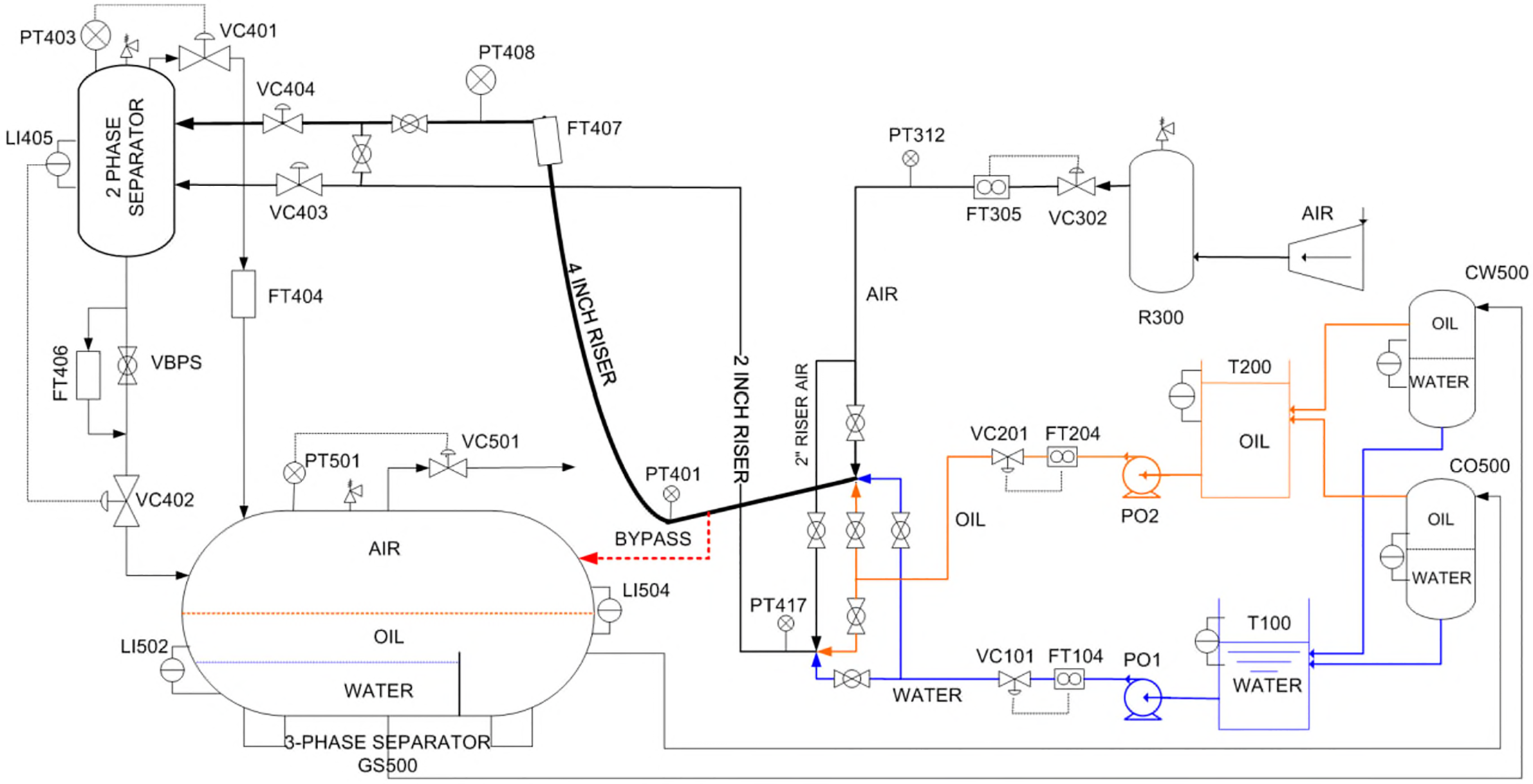
Figure 3: Sketch of the three-phase flow facility

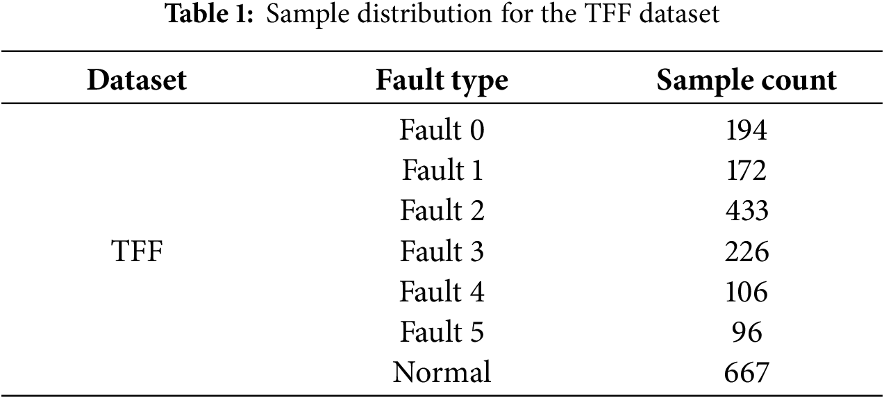
The dataset includes normal operation data as well as data corresponding to six fault types that may arise in real-world operations, with the number of samples for each fault type provided in Table 1. The data is collected under both steady-state and varying conditions, ensuring that it captures a wide range of system behaviors. The sensors sample data at a frequency of 1 Hz, providing detailed information on system performance over time. In this experiment, we segment 50 s of data for each sample.

For fault data collection, the TFF system initially operates in a normal state. Faults are then injected into the system, and the faults develop progressively from minor to severe. Once the fault condition reaches a predefined threshold, fault injection is stopped, and the system is allowed to gradually return to normal. This process creates data that includes the transition from normal to fault states, as well as the recovery from faults, providing valuable information for fault detection and diagnosis models.

This fault injection strategy ensures that the dataset contains a variety of fault conditions and normal operation data, allowing for a comprehensive evaluation of fault detection algorithms. The data is structured in a way that supports training, validation, and testing of models that aim to detect and diagnose faults in pressurized systems.

3.2 Experimental Setup

3.2.1 Baseline Methods

To comprehensively evaluate the effectiveness of the proposed method, we compare it against four representative baseline methods, including GCN [16], GAT [23], IAGNN [24] and GraphSAGE [25]. The selected methods are as follows:

1.   GCN: GCN learns feature representations from graph-structured data, enabling effective processing of data in non-Euclidean spaces.

2.   GAT: GAT uses attention mechanisms to assign different weights to neighboring nodes, enabling efficient and flexible feature aggregation on graph-structured data without requiring prior knowledge of the graph topology.

3.   IAGNN: IAGNN models sensor interactions as multiple edge types in a heterogeneous graph, extracts features from each subgraph using separate GNNs, and fuses them via weighted summation to form the final fault representation.

4.   GraphSAGE: GraphSAGE is an inductive framework that generates node embeddings by sampling and aggregating features from local neighborhoods, enabling generalization to unseen nodes and graphs.

3.2.2 Experimental Setup and Evaluation Indicators

We adopt a 10-fold cross-validation strategy to ensure a more reliable and statistically robust evaluation of the proposed method. Specifically, we first split 10% of the entire dataset as the fixed test set. The remaining 90% of the data is further partitioned into training and validation subsets with an 8:2 ratio under a 10-fold cross-validation scheme. For each fold, the model is trained on the corresponding training subset and validated on the associated validation subset. We repeat the complete training and evaluation process across all 10 folds and report the averaged results in Table 2. All the visualizations of the experimental results presented below, including Figs. 4–9, are based on the first fold of the 10-fold cross-validation.

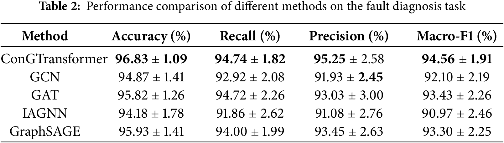
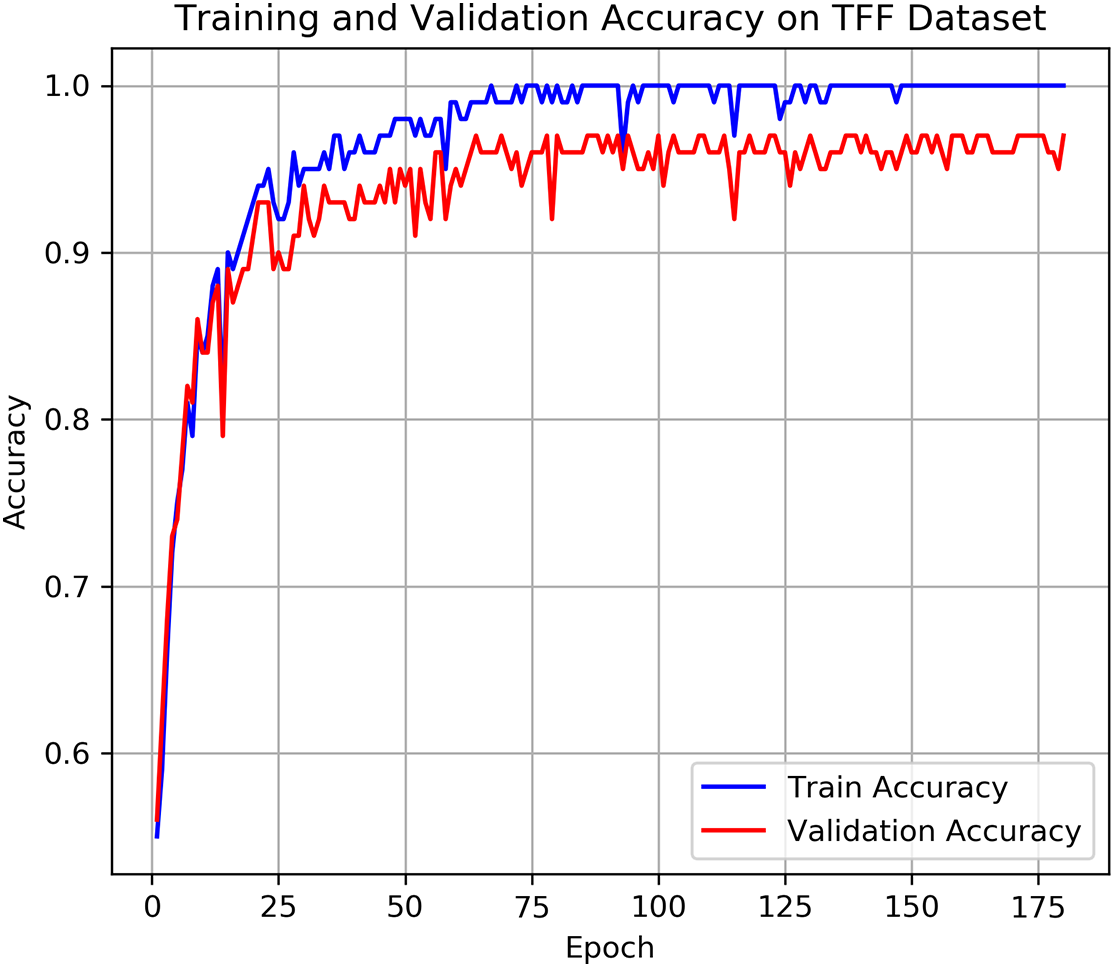
Figure 4: Training and validation accuracy on TFF dataset

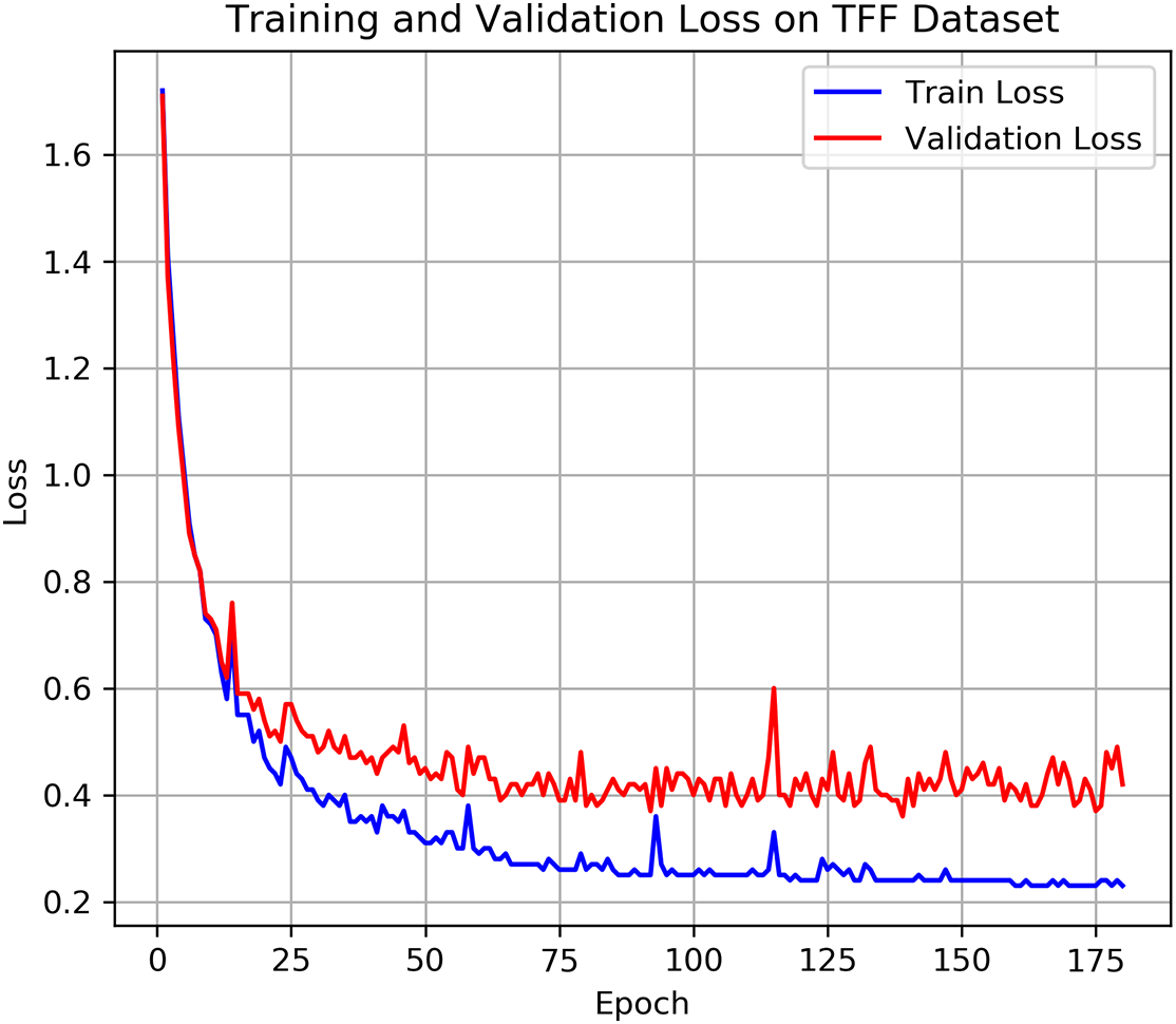
Figure 5: Training and validation loss on TFF dataset

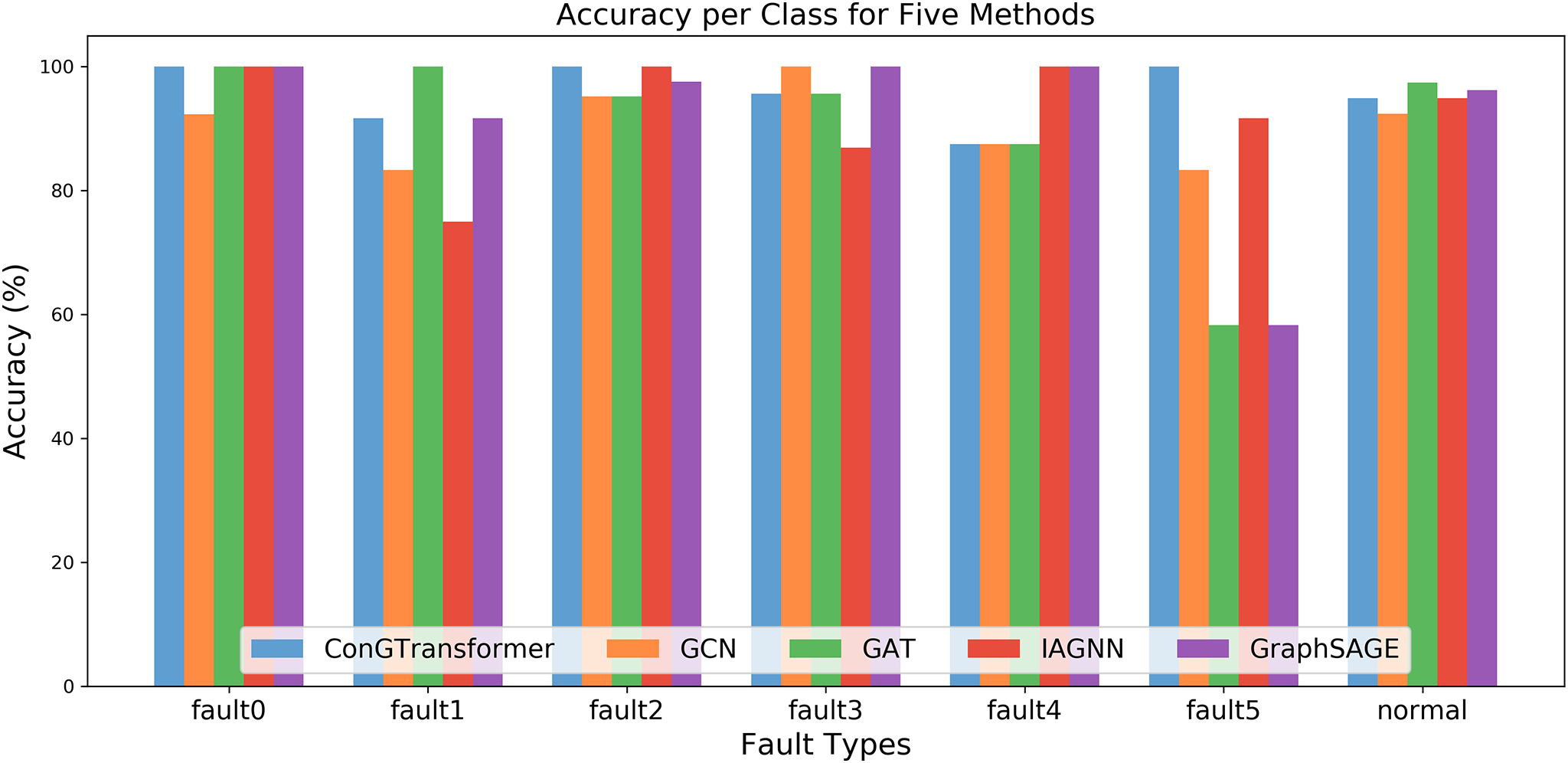
Figure 6: Accuracy per class for five methods

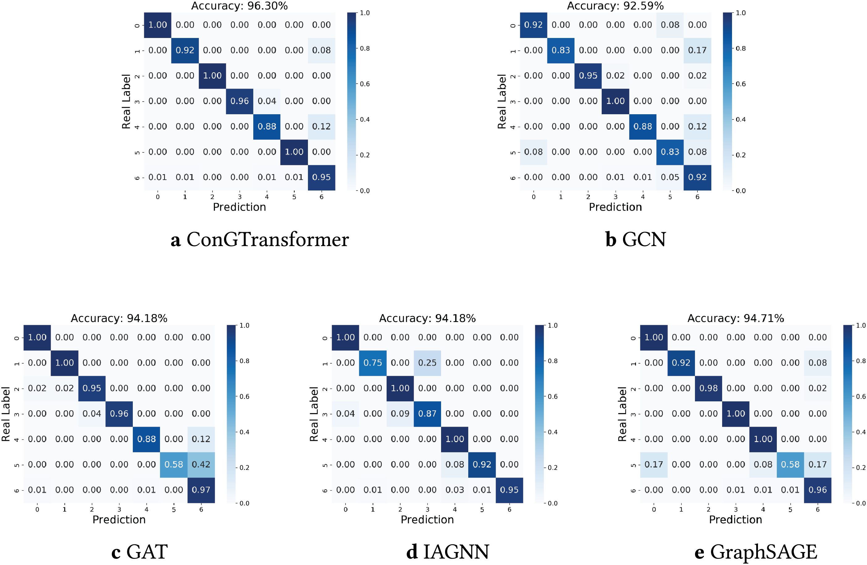
Figure 7: Confusion matrices of different methods: (a) ConGTransformer, (b) GCN, (c) GAT, (d) IAGNN, (e) GraphSAGE

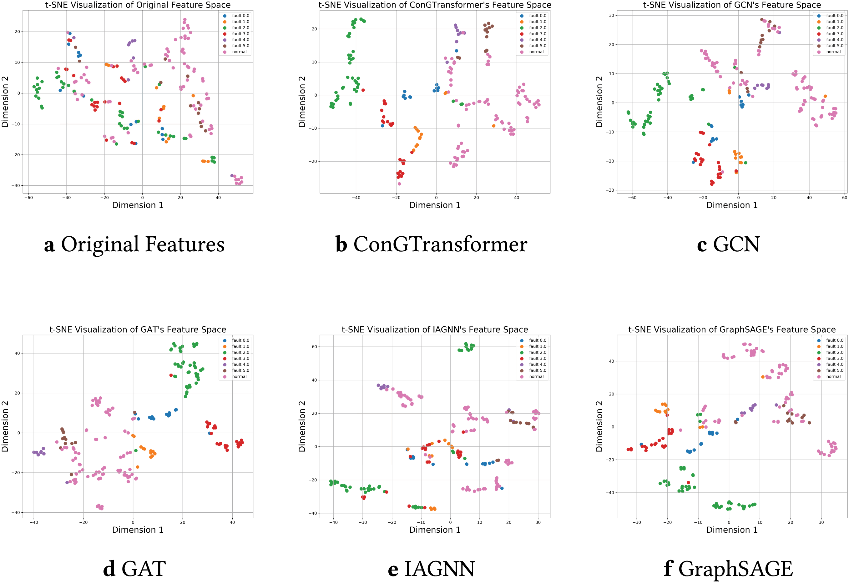
Figure 8: t-SNE visualizations of the feature space for original data and different methods. (a) Original features. (b) ConGTransformer. (c) GCN. (d) GAT. (e) IAGNN. (f) GraphSAGE

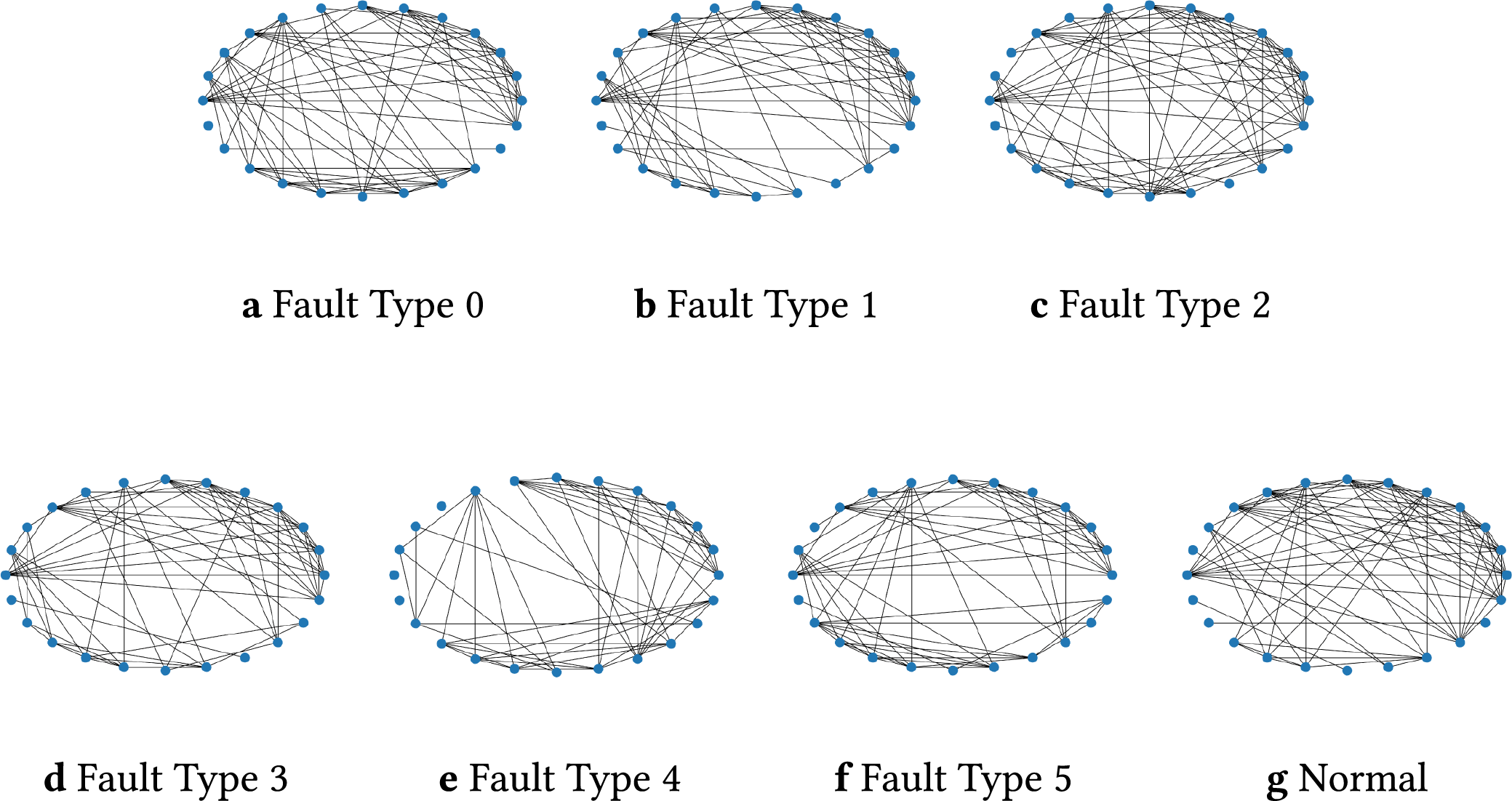
Figure 9: Graph topologies of sensor interactions under the normal condition and six different fault types. Each graph consists of 24 sensor nodes with varying edge structures reflecting different operating or fault conditions: (a) fault type 0; (b) fault type 1; (c) fault type 2; (d) fault type 3; (e) fault type 4; (f) fault type 5; (g) normal condition

To evaluate model performance, we adopted standard metrics including Accuracy, Recall, Precision, Macro-F1 and the confusion matrix. In addition to comparative analysis, an ablation experiment was conducted to assess the impact of the consistency loss.

To determine the optimal hyperparameters for achieving the best performance, we conducted extensive experiments on the proposed ConGTransformer model as well as various baseline methods. As a result, during training, the learning rate was set to 0.001, the hidden dimension to 128, the batch size to 128, the number of layers to 3, and the maximum number of epochs to 200. The dropout rate was fixed at 0.2, and the consistency loss weight λ was set to 0.2.

All experiments were performed on a high-performance computing platform equipped with an AMD EPYC 7763 CPU running at 2.45 GHz (128 cores, 256 threads), an NVIDIA GeForce RTX 4090 GPU with 24 GB memory, and the Ubuntu 20.04.6 LTS operating system.

3.3 Fault Classification Performance

Figs. 4 and 5 show the training and validation accuracy and loss trajectories of the ConGTransformer model on the TFF dataset, respectively. From these plots, we can observe that the model rapidly improves its performance during the initial epochs and continues to converge, indicating a stable learning process. Table 2 provides a comparison of the classification performance of various models on the TFF dataset. Among the key performance metrics, the Macro-F1 score stands out as an important indicator of classification accuracy. It ensures a balanced evaluation by accounting for all categories, including those with fewer samples, and helps identify areas where the model may perform less effectively. Additionally, Fig. 6 compares the accuracy of different methods across various fault types. This comparison highlights how each model handles different fault categories, providing a clearer picture of their robustness. To further analyze the fault diagnosis performance, we also utilize the confusion matrices obtained during the testing phase. By visualizing these matrices, as shown in Fig. 7, we can gain an intuitive understanding of each model’s performance on fault samples from different categories. This visualization allows for a deeper insight into how well each model distinguishes between different types of faults.

When examining the results, ConGTransformer consistently outperforms all other models in terms of accuracy (96.83 ± 1.09%), recall (94.74 ± 1.82%), precision (95.25 ± 2.58%), and Macro-F1 score (94.56 ± 1.91%). The 10-fold cross-validation results indicate that the proposed method not only achieves the highest accuracy but also exhibits the smallest variability, reflecting its robustness and strong generalization capability.

As shown in Fig. 6, the bar chart clearly indicates that ConGTransformer achieves high accuracy across a wide range of fault types, including faults 1 to 6, as well as the normal condition. This consistency highlights the model’s effectiveness in distinguishing between various fault categories, even those with fewer samples.

The confusion matrices in Fig. 7 illustrate the performance of different methods across fault types. Darker colors indicate higher accuracy: diagonal elements with deeper colors correspond to more accurate predictions, while darker off-diagonal elements reflect higher misclassification rates, indicating that a method struggles to distinguish certain fault types. The proposed ConGTransformer shows deep-colored diagonal elements and light-colored off-diagonal elements, demonstrating its ability to effectively separate fault types and achieve high identification accuracy. In contrast, other methods perform less effectively; for example, GAT performs poorly on fault type 5, achieving only 58% accuracy, with the remaining 42% of samples misclassified as fault type 6.

In Fig. 8, points of the same color represent the same fault type. The original feature space shows scattered distributions, while the proposed ConGTransformer forms well-separated clusters, indicating effective classification. In contrast, baseline methods exhibit overlapping clusters; for instance, IAGNN performs poorly for fault 1, and GAT shows mixed distributions for faults 0, 1, 2 and 3, making it difficult to distinguish between different fault types.

Fig. 9 illustrates the effectiveness of the graph construction method presented in Section 2.2. Although a separate graph is constructed for each sample, the graph structures of samples belonging to the same class exhibit similarity, while significant differences exist between the graph structures of different classes. This provides distinguishable information for fault pattern recognition.

Overall, the results indicate that the consistency loss significantly enhances the model’s ability to generalize, particularly in terms of recall and precision. This underscores the importance of maintaining feature consistency during training to optimize diagnostic performance.

3.4 Ablation Experiment

To evaluate the impact of the consistency loss, we conducted an ablation experiment comparing two versions of the model: GTransformer and ConGTransformer. The results, shown in Table 3, highlight the performance gains achieved by incorporating the consistency loss term.

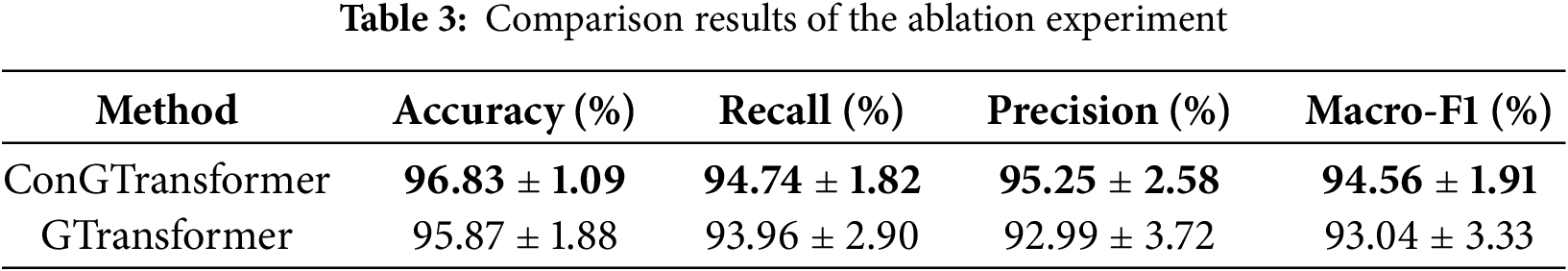
The ConGTransformer model outperforms the baseline GTransformer by enhancing generalization and stability. The introduction of the consistency loss helps maintain feature stability throughout training, leading to improved classification performance and a more balanced precision-recall trade-off. These improvements are reflected in higher evaluation scores, including accuracy, recall, precision, and Macro-F1, further demonstrating the effectiveness of the consistency loss in achieving better fault diagnosis.

4  Conclusions

In this work, we introduced a novel method ConGTransformer for fault diagnosis in complex industrial systems by transforming sensor data into graph-structured representations and applying a Graph Transformer. The method efficiently captures both numerical and relational characteristics of sensor data to provide more accurate and robust fault diagnosis. By incorporating a consistency loss function along with cross-entropy loss, the model ensures that graph representations remain stable across layers while preserving the underlying structural relationships. This approach addresses the challenge of distinguishing between subtle fault types, which is crucial for real-world industrial applications.

Experimental results on the TFF dataset show that the proposed method, ConGTransformer, significantly outperforms existing models in terms of accuracy, recall, precision, and Macro-F1 score. The incorporation of the consistency loss ensures stable and coherent graph representations across layers, which substantially strengthens the reliability of the proposed method for practical industrial fault detection.

We note that there are some limitations in our work. For instance, the current formulation of the consistency loss involves summing over all triplets in the batch, resulting in a computational complexity of O(n3) per layer. While this does not affect inference speed, it increases training overhead, which could be mitigated in future work through more efficient sampling strategies.

Acknowledgement: None.

Funding Statement: This work was partly supported by the National Natural Science Foundation of China under Grants Nos. 62573292, 62206199 and 62476192, National Key Laboratory of Marine Engine Science and Technology under Grant No. LAB-2024-04-WD, Young Elite Scientist Sponsorship Program under Grant No. YESS20220409, the Hainan Province Science and Technology Special Fund under Grant No. ZDYF2024GXJS003, and the Natural Science Foundation of Tianjin under Grant No. 23JCQNJC02010.

Author Contributions: The authors confirm their contributions to the paper as follows: Investigation: Fang Hao and Puyuan Hu; Data curation: Fang Hao and Puyuan Hu; Project administration: Yumo Jiang; Review and editing: Ruonan Liu. All authors reviewed and approved the final version of the manuscript.

Availability of Data and Materials: The datasets analyzed during the current study are openly available in a public repository at MathWorks File Exchange: https://www.mathworks.com/matlabcentral/fileexchange/50938-a-benchmark-case-for-statistical-process-monitoring-cranfield-multiphase-flow-facility, accessed on 01 July 2025.

Ethics Approval: Not applicable.

Conflicts of Interest: The authors declare no conflicts of interest.

References

1. Chang Z, Jia K, Han T, Wei YM. Towards more reliable photovoltaic energy conversion systems: a weakly-supervised learning perspective on anomaly detection. Energy Convers Manag. 2024;316:118845. doi:10.1016/j.enconman.2024.118845. [Google Scholar] [CrossRef]

2. Han T, Xie W, Pei Z. Semi-supervised adversarial discriminative learning approach for intelligent fault diagnosis of wind turbine. Inf Sci. 2023;648:119496. doi:10.1016/j.ins.2023.119496. [Google Scholar] [CrossRef]

3. Yao Y, Han T, Yu J, Xie M. Uncertainty-aware deep learning for reliable health monitoring in safety-critical energy systems. Energy. 2024;291:130419. doi:10.1016/j.energy.2024.130419. [Google Scholar] [CrossRef]

4. Han T, Wang X, Guo J, Chang Z, Chen Y. Health-aware joint learning of scale distribution and compact representation for unsupervised anomaly detection in photovoltaic systems. IEEE Trans Instrum Meas. 2025;74:3538811. doi:10.1109/tim.2025.3571122. [Google Scholar] [CrossRef]

5. Ma L, Dong J, Peng K, Zhang C. Hierarchical monitoring and root-cause diagnosis framework for key performance indicator-related multiple faults in process industries. IEEE Trans Ind Inform. 2018;15(4):2091–100. doi:10.1109/tii.2018.2855189. [Google Scholar] [CrossRef]

6. Liu R, Zhang Q, Lin D, Zhang W, Ding SX. Causal disentangled graph neural network for fault diagnosis of complex industrial process. IEEE Trans Ind Inform. 2024;21(1):386–95. doi:10.1109/tii.2024.3452246. [Google Scholar] [CrossRef]

7. Wang X, Wang H, Peng M. Interpretability study of a typical fault diagnosis model for nuclear power plant primary circuit based on a graph neural network. Reliab Eng Syst Saf. 2025;261:111151. doi:10.1016/j.ress.2025.111151. [Google Scholar] [CrossRef]

8. Chen H, Jiang B, Ding SX, Huang B. Data-driven fault diagnosis for traction systems in high-speed trains: a survey, challenges, and perspectives. IEEE Trans Intell Transp Syst. 2020;23(3):1700–16. doi:10.1109/tits.2020.3029946. [Google Scholar] [CrossRef]

9. Hoang DT, Kang HJ. A survey on deep learning based bearing fault diagnosis. Neurocomputing. 2019;335:327–35. doi:10.1016/j.neucom.2018.06.078. [Google Scholar] [CrossRef]

10. Tao Y, Shi H, Song B, Tan S. A novel dynamic weight principal component analysis method and hierarchical monitoring strategy for process fault detection and diagnosis. IEEE Trans Ind Electron. 2019;67(9):7994–8004. doi:10.1109/tie.2019.2942560. [Google Scholar] [CrossRef]

11. Zhong K, Han M, Qiu T, Han B. Fault diagnosis of complex processes using sparse kernel local Fisher discriminant analysis. IEEE Trans Neural Netw Learn Syst. 2019;31(5):1581–91. doi:10.1109/tnnls.2019.2920903. [Google Scholar] [PubMed] [CrossRef]

12. Liu R, Xie Y, Lin D, Zhang W, Ding SX. Information-based Gradient enhanced Causal Learning Graph Neural Network for fault diagnosis of complex industrial processes. Reliab Eng Syst Saf. 2024;252:110468. doi:10.1016/j.ress.2024.110468. [Google Scholar] [CrossRef]

13. Wu D, Zhao J. Process topology convolutional network model for chemical process fault diagnosis. Process Saf Environ Prot. 2021;150:93–109. doi:10.1016/j.psep.2021.03.052. [Google Scholar] [CrossRef]

14. Wang H, Liu R, Ding SX, Hu Q, Li Z, Zhou H. Causal-trivial attention graph neural network for fault diagnosis of complex industrial processes. IEEE Trans Ind Inform. 2023;20(2):1987–96. doi:10.1109/tii.2023.3282979. [Google Scholar] [CrossRef]

15. Ngo QH, Nguyen BL, Zhang J, Schoder K, Ginn H, Vu T. Deep graph neural network for fault detection and identification in distribution systems. Electr Power Syst Res. 2025;247:111721. doi:10.1016/j.epsr.2025.111721. [Google Scholar] [CrossRef]

16. Kipf TN, Welling M. Semi-supervised classification with graph convolutional networks. arXiv:1609.02907. 2016. [Google Scholar]

17. Xu K, Hu W, Leskovec J, Jegelka S. How powerful are graph neural networks? arXiv:1810.00826. 2018. [Google Scholar]

18. Liu X, Cai Y, Yang Q, Yan Y. Exploring consistency in graph representations: from graph kernels to graph neural networks. arXiv:2410.23748. 2024. [Google Scholar]

19. Shi Y, Huang Z, Feng S, Zhong H, Wang W, Sun Y. Masked label prediction: unified message passing model for semi-supervised classification. arXiv:2009.03509. 2020. [Google Scholar]

20. Dong W, Moses C, Li K. Efficient k-nearest neighbor graph construction for generic similarity measures. In: Proceedings of the 20th International Conference on World Wide Web; 2011 Mar 28–Apr 1; Hyderabad, India. p. 577–86. [Google Scholar]

21. Boutet A, Kermarrec AM, Mittal N, Taïani F. Being prepared in a sparse world: the case of KNN graph construction. In: Proceedings of the 2016 IEEE 32nd International Conference on Data Engineering (ICDE); 2016 Mar 16–20; Helsinki, Finland. p. 241–52. [Google Scholar]

22. Ruiz-Cárcel C, Cao Y, Mba D, Lao L, Samuel R. Statistical process monitoring of a multiphase flow facility. Control Eng Pract. 2015;42:74–88. doi:10.1016/j.conengprac.2015.04.012. [Google Scholar] [CrossRef]

23. Veličković P, Cucurull G, Casanova A, Romero A, Liò P, Bengio Y. Graph attention networks. In: Proceedings of the International Conference on Learning Representations (ICLR); 2018 Apr 30–May 3; Vancouver, BC, Canada. [Google Scholar]

24. Chen D, Liu R, Hu Q, Ding SX. Interaction-aware graph neural networks for fault diagnosis of complex industrial processes. IEEE Trans Neural Netw Learn Syst. 2021;34(9):6015–28. doi:10.1109/tnnls.2021.3132376. [Google Scholar] [PubMed] [CrossRef]

25. Hamilton W, Ying Z, Leskovec J. Inductive representation learning on large graphs. arXiv:1706.02216. 2017. [Google Scholar]