DeepEchoNet: A Lightweight Architecture for Low Resolution Monocular Depth Estimation

1  Introduction

Depth perception is a fundamental cue for understanding and interacting with the physical world. Robots, autonomous agents, and assistive systems benefit from reliable 3D information to navigate cluttered environments, avoid obstacles, manipulate objects, and reason about scene geometry. Traditionally, depth is obtained from active range sensors such as LiDAR or structured-light RGB-D cameras, which directly measure distances to visible surfaces. While highly accurate, these sensors are often expensive, power-hungry, and mechanically fragile, complicating large-scale deployment in low-cost platforms and embedded devices.

In contrast, monocular RGB cameras are cheap, compact, and ubiquitous, which motivates predicting dense depth from a single RGB image (monocular depth estimation). Methodologically, progress accelerated with deep learning, starting from early multi-scale CNN models [1]. More recent approaches leverage transformer backbones and mixed-supervision/scale-robust objectives to improve both accuracy and cross-domain generalization [2–4].

Deep learning has substantially improved monocular depth prediction quality on standard benchmarks such as NYU Depth v2 [5], and more recent transformer-based and hybrid CNN-transformer designs further advanced dense prediction by modeling long-range dependencies [2,6,7]. However, most existing approaches implicitly assume relatively high-resolution inputs (e.g., 480p or higher) and mid- to high-capacity backbones. In embedded or resource-constrained settings, memory and compute budgets are tight, and bandwidth limitations may enforce aggressive compression or downsampling of the input stream. In these scenarios, systems may operate with low resolution imagery such as 96×96 pixels, where high-frequency details are lost and geometric information becomes more ambiguous. We adopt 96×96 as a representative operating point, as it provides a practical compromise between efficiency and fidelity: it is sufficiently small to enable fast and lightweight inference on constrained hardware, while still preserving enough spatial structure to retain meaningful geometric cues, unlike more aggressive reductions (e.g., 64×64). Conversely, higher resolutions (e.g., 128×128) offer increased detail but incur a non-negligible computational and memory overhead that conflicts with strict efficiency targets. Naively resizing high-resolution MDE models to such resolutions often leads to severe accuracy degradation or unstable training. Given these premises, this paper aims to demonstrate that a lightweight neural architecture for monocular depth estimation can operate natively at low resolutions while still yielding useful depth maps on standard indoor benchmarks. Rather than treating low resolution as an afterthought through post-hoc compression, we impose it as a first-class design constraint and tailor both the architecture and the training pipeline to this regime.

We emphasize that the target resolution itself (96×96) is not claimed as a standalone technical novelty, since any existing MDE model can in principle be executed on downsampled inputs. Instead, our contribution is to treat low resolution as a first-class design constraint and to co-design architecture and training accordingly. As evidenced by our baseline study at the same 96×96 input size (Table 1), a straightforward reshaping of a lightweight MobileViT encoder-decoder (MobileViT_Base) or a direct adaptation of a strong mobile baseline (METER-S) yields significantly weaker accuracy than our design that prioritizes low resolution, despite comparable model sizes. This highlights that the 96×96 regime introduces specific failure modes and trade-offs (e.g., downsampling placement, skip fusion, and context injection) that require dedicated design choices rather than naive scaling.

In contrast, we treat low resolution as a primary constraint. Following our analysis, the core motivation is to enable depth-aware perception in embedded and bandwidth-limited scenarios where high-resolution processing is impractical.

Within the context of lightweight MDE under strict resolution constraints, the contributions of this work are as follows:

•   Design regime centered on low resolution. We study monocular depth estimation under a strict 96 × 96 input budget and highlight why naive downsizing of lightweight architectures is often insufficient in this setting.

•   DeepEchoNet architecture for low resolution MDE. We propose a compact hybrid encoder-decoder built on MobileViT [8] and inverted residual blocks [9], coupled with a guided multi-scale decoder with lightweight skip recalibration (scSE) [10] and Atrous Spatial Pyramid Pooling (ASPP)-Lite context refinement.

•   Training pipeline tailored to low resolution inputs. We design a joint RGB-depth pre-processing and augmentation pipeline, including a strong-to-weak schedule, that preserves geometric consistency while improving robustness at low resolution.

•   Empirical validation on NYU Depth v2. We evaluate DeepEchoNet on NYU Depth v2 [5], compare against adapted mobile baselines (including METER [11]) at the same resolution, and provide ablations to quantify the impact of key components.

The rest of the paper is organized as follows: Section 2 reviews the related literature, contrasting heavy-weight depth estimation models with efficient lightweight architectures. Section 3 details the proposed DeepEchoNet framework, including the encoder-decoder design and the training objective. Section 4 describes the experimental setup, covering the dataset, preprocessing pipeline, and implementation details. Section 5 presents the quantitative and qualitative results, comparing the proposed method against baselines and analyzing component contributions through ablation studies. Finally, Section 6 summarizes the main findings and concludes the paper.

2  Related Work

Backbones and dense prediction patterns in MDE. Modern monocular depth estimation (MDE) builds on encoder-decoder dense prediction designs, where skip connections help recover spatial detail and multi-scale context modules enlarge the effective receptive field. U-Net-style skip fusion [12] and atrous spatial pyramid pooling (ASPP) [13] remain common building blocks in depth decoders and refiners. Recent hierarchical transformers such as Swin [3] provide an efficient backbone for dense prediction, and have been widely adopted (directly or via pretrained encoders) in modern depth models [2].

High-capacity and foundation-style MDE models. Early supervised MDE methods demonstrated that deep models can learn metric scene geometry from RGB-D data; a representative milestone is the multi-scale CNN of Eigen et al. [1] on NYU Depth v2 [5]. In the 2021-2024 literature, transformer-based depth estimators improved global context modeling and transfer: DPT [2] adapts transformer backbones for dense prediction, while LeReS-style mixed-supervision training addresses scale/shift issues to recover more realistic scene shape [4]. Structured reasoning has also returned in modern form: NeWCRFs [14] uses neural window fully-connected CRFs as a decoder to refine monocular depth. In parallel, hybrid global-local designs such as GLPDepth (Global-Local Path Networks for Monocular Depth Estimation) [15] target strong accuracy on indoor benchmarks.

Another influential direction reformulates depth estimation as structured classification/ordinal regression over discretized depth values. AdaBins [16] predicts adaptive global bin centers and per-pixel assignments, while LocalBins [17] extends this idea by learning local depth distributions. PixelFormer [18] further explores attention-based skip fusion and ordinal/binning formulations within an encoder-decoder design.

Large-scale multi-dataset training has recently moved toward foundation-style depth models. MiDaS v3.1 [19] highlights the value of mixed supervision (relative and metric cues) for cross-domain transfer, ZoeDepth [20] explicitly combines relative and metric depth training, and Depth Anything [21] scales training using large amounts of (pseudo-)labeled data to improve zero-shot robustness. Relatedly, synthetic data generation pipelines (e.g., RGB-D diffusion) can further increase data diversity [22].

Lightweight and efficient MDE models. Lightweight and efficient deep models for deployment on resource-constrained edge platforms have been widely studied beyond depth estimation, especially in classification and detection. For example, MobileOne [23] is a mobile-oriented backbone explicitly designed to optimize real device latency rather than proxy metrics such as FLOPs alone, achieving sub-millisecond inference on a smartphone while remaining effective across multiple vision tasks.

Similarly, MobileDets [24] studies object detection architectures tailored to mobile accelerators, showing that hardware-aware design can improve the latency/accuracy trade-off across different embedded platforms. Finally, models such as EdgeViT [25] and MicroViT [26] have been proposed as lightweight Vision Transformers optimized for edge deployment, achieving a favorable trade-off between accuracy, latency, and energy efficiency through EdgeViT’s Local-Global-Local attention design and MicroViT’s low-complexity, single-head attention mechanism. These works highlight the broader importance of efficiency-driven and hardware-aware model design for real-time vision on edge systems.

A complementary research line focuses on efficiency of MDE solutions, aiming to make MDE feasible under limited compute, memory, and power budgets. Compact encoders based on depthwise separable convolutions and inverted residual blocks (e.g., MobileNetV2) are common starting points for embedded-friendly designs [9]. Hybrid mobile backbones further integrate lightweight self-attention: MobileViT [8] combines local convolutions with transformer blocks operating on small patch sequences. For self-supervised settings on edge devices, Lite-Mono [27] demonstrates that a careful CNN-transformer hybrid can retain accuracy with substantially fewer parameters.

Beyond backbones, decoder design and feature fusion strongly impact compact models. Lightweight feature recalibration mechanisms such as concurrent spatial and channel squeeze-excitation (scSE) [10] improve skip fusion by emphasizing informative channels and spatial locations. Guided decoding strategies [28] filter or gate skip connections before fusion, improving the balance between global bottleneck context and local detail while remaining efficient.

Among lightweight supervised MDE approaches, METER [11] is a key reference for this work. METER targets embedded platforms by combining a MobileViT-style encoder with a light decoder and a training pipeline designed for efficient monocular depth estimation, reporting strong results on NYU Depth v2 [5]. Moreover, it proved to be an adaptable baseline for further optimizations [29–31].

Training objectives and supervision paradigms. Most supervised MDE pipelines treat depth as dense regression and optimize point-wise losses (e.g., ℓ1/ℓ2) combined with regularizers that preserve structure. Scale-aware and scale/shift-robust formulations were introduced early [1] and are refined in modern mixed-supervision pipelines that incorporate normalization and geometry cues (e.g., normal-based terms) [4]. Structural similarity (SSIM) [32] is often used as an additional signal to preserve local structure; it is widely adopted in self-supervised photometric objectives (e.g., ManyDepth [33] and Lite-Mono [27]) and also appears in composite supervised losses such as the BLF in METER [11]. Alternative re-weighting strategies such as focal loss [34] have been explored to emphasize hard pixels, though their effect in low resolution depth can be mixed. On the architecture side, transformer feed-forward blocks have also been augmented with gated MLP variants (e.g., GLU/GEGLU) motivated by transformer literature [35]. More recently, diffusion-based and generative formulations (e.g., DepthGen [36]) introduce probabilistic objectives that model depth as a conditional distribution rather than a deterministic regression target, enabling better uncertainty estimation and robustness to ambiguous regions.

Positioning of this work. High-capacity transformer and foundation-style models [2,21] demonstrate the benefits of strong global context and large-scale training, but are typically designed for higher resolutions and larger compute budgets. Lightweight hybrids based on MobileNet family models [37], MobileViT [8], and METER [11] show that useful depth maps can be obtained under tighter constraints, but generally still assume medium-resolution inputs. In this work, we focus on the low resolution regime (96×96) and study architectural choices (e.g., downsampling placement, skip fusion, and context injection) that remain effective under a severely limited spatial budget.

3  Proposed Method

3.1 Problem Formulation and Notation

We consider supervised monocular depth estimation from a single RGB image. Given an RGB input I∈R3×H×W, the goal is to predict a dense depth map D^∈R1×H×W, trained against ground truth D. In this work, we focus on native low resolution inputs with H=W=96, and we express depth values in centimeters. Depth is clamped to a valid range [Dmin,Dmax] with Dmin=50 cm and Dmax=1000 cm, as indicated by the considered benchmark.

3.2 Baselines Considered

Before introducing DeepEchoNet, we summarize the baselines used in this work to compare our solution. Both baselines are lightweight encoder-decoder networks built on MobileViT-style encoders [8,11] and adapted to operate directly at low input resolution.

METER-S METER follows an encoder-decoder design with skip connections. The encoder alternates MobileNetV2-style inverted residual blocks [9] with MobileViT blocks [8], enabling efficient local feature extraction and lightweight global context modeling. The decoder fuses multi-scale features through lightweight upsampling and skip connections, producing a dense depth map. In this work, METER-S is adopted both as the primary lightweight reference model [11] and as the starting architecture upon which our framework is built.

MobileViT_Base In addition to METER, we introduce another baseline MobileViT-inspired model (MobileViT_Base) that simplifies the encoder and restructures the decoder to better match the spatial scales encountered in the low resolution regime. This baseline helps isolate architectural choices that matter most when operating at 96×96, highlighting the impact of DeepEchoNet design.

3.3 DeepEchoNet Architecture

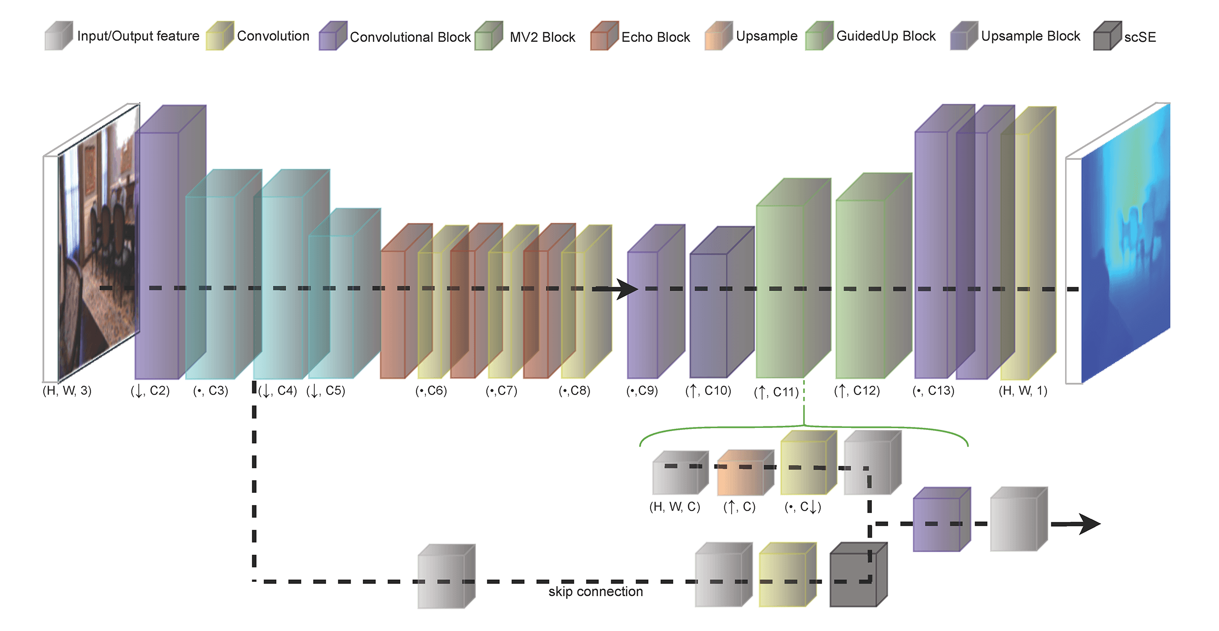
DeepEchoNet targets monocular depth estimation at native resolutions of 96 × 96. At this low resolution regime, local texture cues are heavily degraded and depth prediction benefits from incorporating wider contextual information to reduce ambiguities in indoor scenes. For this reason, the model retains the hybrid design of MobileViT [8], combining efficient convolutional feature extraction with lightweight transformer blocks that enable global feature mixing at modest overhead (the token grid is small at 96×96). This choice also keeps the comparison with mobile baselines such as METER [11] meaningful, allowing us to isolate the contribution of the proposed decoder and training pipeline under a consistent encoder family. We augment the encoder with a guided decoder that selectively fuses multi-scale skip features. An overview is shown in Fig. 1.

Figure 1: Overview of the DeepEchoNet architecture. The encoder combines MobileNetV2 downsampling [9] with three MobileViT-Echo blocks [8] to produce a compact 12×12 bottleneck. The guided decoder restores spatial resolution using one Upsample block and two GuidedUpSample blocks, which fuse decoder features with scSE-recalibrated encoder skips [10] via separable convolutions. A final fusion with the shallow skip and an ASPP-Lite module [13] refine the prediction before the last convolution outputs the depth map.

3.3.1 Encoder Design

The DeepEchoNet encoder is a MobileViT-inspired backbone designed for low resolution inputs. Given a 96×96 RGB image, the encoder applies the following sequence:

1.   Convolutional stem. A first convolutional block (conv1) with stride 2 reduces the resolution from 96×96 to 48×48 and expands the channel dimension from 3 to C0=12. The block follows a Conv-BN-ReLU-Conv pattern, where a 3×3 convolution is followed by a 1×1 projection.

2.   Inverted residual blocks. Three MobileNetV2-style inverted residual blocks [9] progressively increase capacity while downsampling:

      •   mv2_1: 48×48, C0→C1=24 (stride 1),

      •   mv2_2: 48×48→24×24, C1→C2=48 (stride 2),

      •   mv2_3: 24×24→12×12, C2→C3=96 (stride 2).

Each block uses an expansion factor to form a depthwise separable convolutional core, followed by a linear projection back to the output channels, and employs residual connections when shapes match [9].

3.   MobileViT stages with bridges. Starting from the 12×12 feature map with C3=96 channels, the encoder applies three MobileViT blocks [8] with bridge projections:

      •   mvit1: 12×12,C3→C3,

      •   bridge12: 12×12,C3→C4=144,

      •   mvit2: 12×12,C4→C4,

      •   bridge23: 12×12,C4→C5=192,

      •   mvit3: 12×12,C5→C5.

Each MobileViT block refines features locally via convolutions, projects them to a latent dimension, unfolds into small 2×2 patches, applies a lightweight transformer (multi-head self-attention [38] and MLP) to model global interactions, and then folds tokens back into a spatial feature map fused with the convolutional features [8]. The bridge layers are 1×1 Conv-BN-ReLU projections that adjust channel widths between successive stages.

4.   Bottleneck projection. A final 1×1 convolutional block (conv2) maps the output of mvit3 from C5=192 to C6=224, producing the bottleneck feature map Fbottleneck∈RC6×12×12.

In addition to the bottleneck, the encoder exposes intermediate feature maps that act as skip connections in the decoder, enabling multi-scale reconstruction while preserving low-level structure despite the limited spatial resolution.

3.3.2 Guided Decoder and Skip Fusion

The decoder reconstructs a dense depth map at 96×96 from the 12×12 bottleneck while exploiting multi-scale information from encoder skips. A core goal is to fuse global context and local structure effectively while remaining computationally lightweight. As illustrated in the architecture overview figure, DeepEchoNet uses: (i) hierarchical upsampling with bilinear interpolation and separable convolutions; (ii) guided skip fusion with scSE-based recalibration [10]; and (iii) an ASPP-Lite module [13] for multi-scale context aggregation near the output.

Concretely, the decoder first applies a 1×1 projection (conv_in) to reduce the bottleneck channels, and then performs three upsampling stages: one unguided fusion stage and two guided fusion stages in the spirit of guided decoders for MDE [28]. Each guided fusion block operates as follows:

1.   Decoder projection: bilinearly upsample the current decoder feature and project it to Cout channels with a 1×1 convolution + BN.

2.   Skip recalibration: project the corresponding skip feature to Cout channels and apply scSE recalibration [10].

3.   Fusion: concatenate the projected decoder and recalibrated skip features and fuse them with a separable convolution + BN + ReLU [9].

After reaching 96×96, a final fusion with the shallow skip is followed by ASPP-Lite with dilation rates 1/2/3 [13], and the final convolution produces the depth prediction.

3.4 Training Objective

DeepEchoNet is trained in a fully supervised fashion using the balanced loss function (BLF) introduced in METER, with an added, custom Gradient-based edge loss. The goal is to combine a robust pixel-wise depth regression term with additional components that promote sharp edges, geometrically consistent surfaces, and structural similarity between predicted and ground-truth depth maps.

Let D^∈R1×H×W denote the predicted depth map and D∈R1×H×W the ground-truth depth, both expressed in centimeters and clamped to [Dmin,Dmax]. The BLF used in this work is:

ℒ=ℒdepth+λ1ℒgrad+λ2ℒnorm+λ3ℒSSIM,(1)

where λ1, λ2, and λ3 are scalar weights.

Depth regression term

A primary component is a pixel-wise ℓ1 loss over valid pixels:

ℒdepth=1T∑i∈Ω∗|d^i−di|,(2)

where Ω∗ is the set of valid pixels, T=|Ω∗|, and d^i,di are predicted and ground-truth depths at pixel i.

Gradient-based edge loss

To emphasize depth discontinuities and small structures, we include a gradient consistency term inspired by supervised MDE objectives [1,11,39]. Both predicted and ground-truth depth maps are passed through a fixed Sobel operator to obtain horizontal and vertical gradients, and their differences are penalized:

ℒgrad=1T∑i∈Ω∗(|∂xd^i−∂xdi|+|∂yd^i−∂ydi|).(3)

This encourages the predicted depth map to share the same edge structure as the ground truth, reducing over-smoothed boundaries. Surface normals are approximated from depth gradients:

nD=(−∂xD,−∂yD,1),nD^=(−∂xD^,−∂yD^,1),

and a cosine penalty is applied:

ℒnorm=1T∑i∈Ω∗(1−cos⁡(nD^,i,nD,i)),(4)

promoting geometrically consistent surfaces.

Structural similarity

To encourage structural agreement between depth maps, a structural similarity term is included:

ℒSSIM=1−SSIM(D^,D),(5)

where SSIM is computed between the predicted and ground-truth depth maps [32] and is commonly used within depth estimation objectives [11,40].

3.5 Low Resolution Pre-Processing and Augmentation

RGB images are loaded and converted into 8bit, 3 channels tensors and normalized between [0, 1]. Depth maps may be stored as 8- or 16-bit images; 16-bit depth values are converted to centimeters, while 8-bit depth is linearly mapped to [0, 1000] cm. All depth values are clipped to [Dmin,Dmax] with Dmin=50 cm and Dmax=1000 cm. However, using different depth units (such as meters, or normalizing all values between [0, 1]) do not substantially change the model performances. RGB inputs are optionally normalized with ImageNet statistics [41]. All augmentations operate on paired (I,D) to preserve alignment. A qualitative example is shown in Fig. 2

Figure 2: Qualitative illustration of the joint RGB–depth augmentation pipeline. The first row shows the original RGB image together with two perturbed variants produced by the shifting strategy (gamma/brightness/color scaling). The second row displays the corresponding ground-truth depth maps, where an additional depth shift S={−10,+10} cm is added to simulate sensor bias. The bottom row visualizes zoomed-in patches, highlighting that the augmentation alters appearance while preserving coarse geometry. Larger depths are brighter, smaller depths are darker.

We apply a compact set of geometric and appearance perturbations:

•   Flips: vertical and horizontal flips are applied with fixed probabilities.

•   Channel swap: with a fixed probability, RGB channels are randomly permuted to reduce sensitivity to color statistics.

•   Shifting strategy (in the spirit of [11]): with probability pshift, we apply mild gamma/brightness/color scaling to I and a depth offset Δz∼𝒰(−10,10) cm to D, followed by clipping.

•   Strong-to-weak schedule: during the first half of training we additionally enable a small shared affine transform (rotation ±8∘, scale [0.95,1.05]) and additive Gaussian noise on RGB (σ=0.02); these stronger perturbations are disabled in the second half for refinement.

4  Experimental Setup

4.1 Dataset and Split

All experiments are conducted on the NYU Depth v2 indoor dataset [5], which provides aligned RGB images and depth maps acquired with an RGB-D sensor. In order to perform fair comparison, we adopted the standard evaluation protocol widely used in monocular depth estimation (employed also by our baseline comparison model, METER [11]), with a training set of more than 50,000 RGB-depth pairs and a held-out test set containing 654 images, taken from the NYU Depth v2 dataset.

In addition, we report a cross-dataset evaluation on SUN RGB-D [42] to assess robustness under domain shift, excluding the NYU subset contained in SUN RGB-D.

4.2 Preprocessing and Low Resolution Inputs

We operate in an low resolution regime, resizing RGB and depth to 96×96 pixels. RGB is resized with bilinear interpolation, while depth is resized with nearest-neighbour interpolation to avoid interpolating invalid values. Depth is represented in centimetres and clipped to the physically meaningful interval [50, 1000] cm, as previously specified in the Proposed Method section. During training, we apply the joint RGB-depth augmentation pipeline described in Section 3.5 (including the strong-to-weak schedule); at test time, only deterministic resizing (and optional ImageNet-style normalisation) is applied.

4.3 Training Protocol and Hyperparameters

All models are trained in a fully supervised fashion using the balanced loss function in Section 3.4 (point-wise ℓ1 depth regression, gradient alignment, normal consistency, and SSIM-based similarity). Unless otherwise stated, the SI-log and focal-loss variants explored in this work are not used in the final models.

We use the AdamW optimizer [43] with learning rate η0=10−3, momentum parameters (β1,β2)=(0.9,0.999), and weight decay λ=0.01. The batch size is 256 without gradient accumulation. The learning rate is controlled by a ReduceLROnPlateau scheduler monitoring the validation Absolute Relative Error (AbsRel), with: (i) mode = min, (ii) factor 0.5, (iii) patience 5 epochs, threshold 10−4, (iv) cooldown 2 epochs, and (v) minimum learning rate 10−6. The number of training epochs is not fixed. At each epoch, we evaluate on the validation subset, keep the checkpoint with the lowest validation AbsRel, and apply an early stopping procedure when AbsRel does not improve for Pstop consecutive epochs, with Pstop equal to 30. The number of training epochs performed with this approach is around 70 epochs.

4.4 Evaluation Metrics

Metrics are computed over valid pixels Ω∗ (where ground-truth depth is available and within the evaluation range), with T=|Ω∗| [1,2,39]. Let di and d^i denote ground-truth and predicted depth at pixel i∈Ω∗. We report RMSE and MAE (in centimetres), AbsRel, and the standard threshold accuracies δk at τ∈{1.25,1.252,1.253} [1]:

AbsRel=1T∑i∈Ω∗|d^i−di|di,(6)

MAE=1T∑i∈Ω∗|d^i−di|,(7)

RMSE=1T∑i∈Ω∗(d^i−di)2,(8)

δ(τ)=1T|{i∈Ω∗∣max(d^idi,did^i)<τ}|.(9)

4.5 Hardware and Inference-Time Measurement

Unless otherwise specified, all experiments are run on a Linux workstation equipped with a single NVIDIA GeForce RTX 4070 SUPER GPU and PyTorch framework. The code is publicly available on the Github webpage https://github.com/giuliocapo/DeepEchoNet.

Inference-time measurements are reported in a model-only setting, i.e., we measure the forward-pass latency excluding dataset I/O and preprocessing. Each model is timed with batch size 1 using an input tensor of shape 1×3×H×W (with H=W=96 for the main experiments). Before timing, we perform several warm-up forward passes to stabilise GPU clocks. We then run N repeated forward passes and compute the average time per frame:

tframe=total timeN,FPS=1tframe.

All reported FPS values refer to this single-image, single-GPU setting.

5  Results

5.1 Quantitative Results

5.1.1 Comparison with Baseline Models

We compare DeepEchoNet with two MobileVIT models at the same input resolution. More in detail, our comparison includes: (i) METER-S adapted to 96×96 by adjusting padding and cropping so that MobileViT patching remains valid, (ii) MobileViT_Base, a reshaped MobileViT-based encoder-decoder baseline at 96×96, and (iii) the final DeepEchoNet configuration with all the implemented improvements, such as guided decoding (GD), widened encoder tail (WE), squeeze-and-excitation module on skip connections (scSE), and ASPP-Lite refinement block (ASPP-lite).

The comparison results are shown in Table 1. Although MobileViT_Base is more compact than METER-S, its performance is slightly worse across all error metrics (e.g., AbsRel 0.205 vs. 0.195, RMSE 69.00 vs. 67.49 cm, and MAE 52.53 vs. 51.92 cm), indicating that reshaping the architectural hierarchy to match low resolution scales is not sufficient by itself. This trend is also reflected in the accuracy thresholds, where MobileViT_Base shows marginally lower δ2 and δ3 values, suggesting a less consistent depth estimation quality over broader tolerance ranges.

In contrast, DeepEchoNet achieves the best overall accuracy. AbsRel is reduced to 0.186, while RMSE and MAE decrease to 63.56 and 48.18 cm, respectively, indicating improvements both in global error and average per-pixel deviation. Moreover, δ1 improves from 0.673 (METER-S) to 0.720, and gains are also observed for δ2, while δ3 remains on par with the strongest baseline. This suggests that DeepEchoNet not only improves strict accuracy but also preserves robustness at looser error thresholds, achieving a more reliable depth prediction overall. Notably, these improvements are obtained while using fewer parameters than METER-S.

Regarding inference times, DeepEchoNet improves runtime performance with respect to the main baseline METER-S, reaching approximately 240 FPS compared to 220 FPS. This demonstrates that the proposed architectural refinements not only enhance accuracy but also lead to faster inference. The fastest model remains MobileViT_Base at approximately 280 FPS, reflecting the expected trade-off between extreme compactness and depth estimation accuracy.

5.1.2 Cross-Dataset Robustness on SUN RGB-D

We added a cross-dataset robustness evaluation on SUN RGB-D [42] to assess generalization beyond NYU Depth v2. Since SUN RGB-D is not provided with an official test split for monocular depth estimation, we randomly sampled 600 frames (fixed seed), excluding the NYU subset included in SUN RGB-D to prevent any overlap with the training distribution. Depth maps were decoded following the official SUNRGBD toolbox (bit operation + metric conversion) and evaluation was limited to the 0.5–8 m range (consistent with the toolbox clipping). As expected, all models exhibit a domain-shift degradation; however, Table 2 shows that DeepEchoNet consistently outperforms both the adapted METER-S baseline and the MobileViT_Base baseline on RMSE/MAE and δ-accuracies, indicating stronger cross-dataset robustness. This trend is also supported by the qualitative comparison in Fig. 3, where DeepEchoNet produces sharper predictions and better preserves scene structures (e.g., object boundaries and thin elements), while METER-S tends to generate smoother and less detailed depth maps under the same domain shift; we report qualitative results against METER-S as it is the strongest baseline on SUN RGB-D among the evaluated lightweight variants.

Figure 3: Qualitative comparison on SUN RGB-D: DeepEchoNet vs. METER-S. From left to right, the images are the input RGB, the ground truth, the DeepEchoNet prediction and the METER-S prediction respectively. In particular, DeepEchoNet produces predictions with sharper details with respect to METER-S.

5.1.3 Noise Sensitivity on NYU Depth v2

We further test robustness to input perturbations on DeepEchoNet by adding zero-mean Gaussian noise with standard deviation σ=0.02 to the RGB input (in [0, 1]) at test time, before normalisation. Table 3 shows that performance degrades smoothly compared to the clean test set, indicating limited sensitivity to moderate sensor noise at the target 96×96 resolution.

In addition, Fig. 4 reports a challenging indoor scene with heavy clutter and repeated fine-scale structures, where monocular cues become less informative at 96×96 and the prediction tends to oversmooth depth discontinuities.

Figure 4: Qualitative example on NYU Depth v2 under additive Gaussian RGB noise (σ=0.02) at 96×96 resolution. From left to right: perturbed RGB input, DeepEchoNet prediction, and ground-truth depth (magma colormap; brighter = farther).

5.1.4 Ablation Results

To better understand which design choices contribute most to the final performance, we perform ablation experiments deactivating several DeepEchoNet modules. Unless otherwise noted, variants are trained from scratch on NYU Depth v2 [5] with the same optimiser, learning-rate scheduler, and base augmentation pipeline; differences concern architecture or loss configuration.

The first block of Table 4 isolates the contribution of architecture and augmentation (enabled for all experiments, but “no-agumentation” one). Adding the guided decoder improves performance (AbsRel 0.205→0.200, δ1 0.675→0.685) while remaining lightweight; in our implementation, guided fusion combines bilinear upsampling and separable convolutions with skip recalibration, improving the alignment between global bottleneck context and local encoder detail [10]. The largest accuracy jump is obtained by combining guided decoding with encoder widening, ASPP-Lite, and scSE-based skip recalibration, reducing AbsRel to 0.189 and increasing δ1 to 0.706. Further widening provides a smaller but consistent improvement (AbsRel 0.188, δ1=0.711). We also tested the best variant with disabled data augmentation schema (5th row). As expected, the generalization capabilities of the model degraded, with worse performances on all evaluated metrics. Finally, enabling the strong-to-weak augmentation schedule yields the best result (AbsRel 0.186, δ1=0.720), further improving the metrics with respect to previous best configuration.

The second block summarises additional variants, taken from most popular MDE models, that proved to not improve accuracy in this setting. In particular, Auxiliary multi-scale heads combined with a scale-invariant log loss (SI-Log) [1] yield worse metrics and tend to produce over-regularised predictions. A focal re-weighting of the ℓ1 depth term inspired by focal loss [34] also degrades global performance. Replacing the standard feed-forward block with a GEGLU variant [35] converges stably but underperforms the baseline. Finally, nearest-neighbour upsampling slightly worsens RMSE and AbsRel, confirming that bilinear upsampling plus convolution provides a better sharpness-aliasing trade-off at 96×96.

To improve transparency on training dynamics, Fig. 5 reports the training loss, validation AbsRel, and the learning-rate evolution under ReduceLROnPlateau for the final DeepEchoNet configuration. The curves show stable convergence without divergence, and learning-rate reductions align with validation plateaus; we select the final checkpoint by validation AbsRel. Sensitivity to the loss design and augmentation strength is further discussed via the ablation study (Table 4), where more complex loss variants do not yield consistent gains, while the strong-to-weak augmentation schedule provides a measurable improvement.

Figure 5: Training and validation curves for the final DeepEchoNet configuration on NYU Depth v2 at 96×96 resolution, including the ReduceLROnPlateau learning-rate schedule.

5.2 Qualitative Results

Quantitative metrics provide a compact summary but are not enough to fully capture the perceptual quality of the predicted depth maps. We therefore report qualitative examples on NYU Depth v2 [5]. All depth predictions are single-channel real-valued maps. For qualitative visualisation, both ground-truth and predicted depth maps are clamped to a fixed depth range, linearly normalised to [0, 1], and mapped to RGB using a perceptually uniform sequential colormap. Despite the extremely low input resolution, DeepEchoNet recovers the main planar structures of indoor scenes (walls, floor, large furniture) and delineates many object boundaries and depth discontinuities (Fig. 6).

Figure 6: Qualitative examples of DeepEchoNet predictions on NYU Depth v2 at 96×96 resolution. For each scene we show (left to right) the RGB input, the ground-truth depth map, and the DeepEchoNet prediction. Larger depths are brighter, smaller depths are darker.

A direct depth-map comparison for the same test image is shown in Fig. 7. Consistently with the quantitative analysis, DeepEchoNet produces sharper boundaries and fewer artefacts along depth discontinuities than the baselines.

Figure 7: Direct comparison of predicted depth maps for the same NYU Depth v2 scene at 96×96 resolution. From left to right: METER-S (adapted), MobileViT_Base baseline, and final DeepEchoNet prediction. Larger depths are brighter, smaller depths are darker.

Finally, Fig. 8 illustrates typical failure modes for the auxiliary multi-scale + SI-Log variant: predictions become over-regularised and overly smooth, with biased estimates on reflective surfaces, textureless regions, and strong occlusions, where monocular cues are intrinsically ambiguous in the low resolution regime [1].

Figure 8: Failure cases on NYU Depth v2 for the auxiliary multi-scale + SI-Log variant, showing over-regularised (oversmoothed) predictions in challenging regions. Larger depths are brighter, smaller depths are darker.

To further characterise the limitations of the final DeepEchoNet model, we additionally report an example of failure case of depth estimation on NYU Depth v2 on Fig. 9. The sample scene is highly cluttered (book stacks and shelves) and contains many small, overlapping objects with sharp depth discontinuities. In this setting, the low resolution regime amplifies the ambiguity of monocular cues: fine structures and thin depth layers are easily lost, and the prediction tends to become over-smoothed. In fact, DeepEchoNet captures the coarse layout but struggles to preserve fine-grained depth transitions under heavy occlusions, leading to a large error in this outlier case. We note, however, that attributing prediction errors to specific image structures in a strictly causal or quantitative manner remains challenging, as current analysis tools for deep models do not provide definitive mechanisms for isolating the exact factors responsible for individual failure modes. Therefore, our analysis is based on consistent empirical trends observed across high-error samples rather than formal causal attribution.

Figure 9: Failure case qualitative example on NYU Depth v2 for the final DeepEchoNet model (selected by per-image RMSE). From left to right: RGB input, DeepEchoNet prediction, and ground-truth depth. Depth maps are clamped to a fixed range, linearly normalised to [0,1], and visualised with a perceptually-uniform sequential colormap (larger depths are brighter).

5.3 Discussion

The experimental analysis supports the following conclusions for low resolution MDE. First, simply adapting existing architectures to 96×96 is insufficient: MobileViT_Base does not outperform METER-S despite having fewer parameters, indicating that low resolution changes the effective trade-offs between depth, width, and downsampling placement. Second, ablations confirm that most gains stem from targeted architectural modifications: guided decoding with skip recalibration, together with a widened encoder tail and ASPP-Lite refinement [10,13], yields consistent improvements, while more complex loss variants can lead to over-regularisation. Finally, the resolution study shows that 96×96 offers a strong operating point: it preserves enough spatial structure to recover indoor geometry while remaining comfortably real-time.

These findings are also reflected in the observed failure modes (Figs. 8 and 9), where errors concentrate in regions requiring fine spatial detail, sharp depth discontinuities, or involving thin and cluttered structures. While such patterns are consistent across high-error samples, providing a more rigorous attribution of these errors to specific input cues remains challenging due to the lack of interpretability techniques. In particular, existing explainability (XAI) methods are not well suited to dense regression tasks such as monocular depth estimation. Algorithms such as Grad-CAM [44], originally developed for classification, require defining an attribution target, which is inherently ambiguous in the case of per-pixel continuous predictions. Developing principled explainability methods for dense depth prediction would therefore be instrumental in better understanding these effects, and represents a promising direction for future work.

6  Conclusion

This work addressed supervised monocular depth estimation (MDE) in an low resolution regime, where the input is a single RGB image downsampled to 96×96 pixels, motivated by depth-aware perception on resource-constrained platforms equipped with low-cost cameras as an alternative or complement to active sensors. We proposed DeepEchoNet, a lightweight hybrid CNN-transformer architecture tailored to operate natively at low resolution. Tested on NYU Depth v2, DeepEchoNet improves over both an adapted METER-S baseline and a reshaped MobileViT_Base baseline, achieving AbsRel 0.186 and δ1=0.720 while maintaining real-time inference (desktop GPU) and remaining in the real-time regime on an embedded device at batch size 1. Moreover, cross-dataset experiments on the SUN RGB-D dataset confirmed the validity of the proposed approach, with DeepEchoNet exhibiting less domain-shift degradation of the counterparts. Future work will extend dataset testing on real-world data acquired with commodity cameras, and will further analyze robustness to sensor noise and image degradations together with representative failure cases. Deployment-oriented improvements such as pruning/quantization and hardware-specific optimisation, as well as self-supervised or semi-supervised signals from stereo or multi-view data, may further improve robustness in challenging low resolution scenarios. Finally, the adaptation of XAI methods to explain the behavior of monocular depth estimation models will be investigated.

Acknowledgement: Not applicable.

Funding Statement: The authors received no specific funding for this study.

Author Contributions: The authors confirm contribution to the paper as follows: study conception and design: Giulio Caporro, Paolo Russo; data collection: Giulio Caporro; analysis and interpretation of the results: Giulio Caporro, Paolo Russo; draft manuscript preparation: Giulio Caporro, Paolo Russo. All authors reviewed and approved the final version of the manuscript.

Availability of Data and Materials: Not applicable.

Ethics Approval: Not applicable.

Conflicts of Interest: The authors declare no conflicts of interest.

References

1. Eigen D, Puhrsch C, Fergus R. Depth map prediction from a single image using a multi-scale deep network. Adv Neural Inf Process Syst. 2014;2:2366–74. [Google Scholar]

2. Ranftl R, Bochkovskiy A, Koltun V. Vision transformers for dense prediction. In: Proceedings of the 2021 IEEE/CVF International Conference on Computer Vision (ICCV); 2021 Oct 10–17; Montreal, QC, Canada. p. 12179–88. doi:10.1109/iccv48922.2021.01196. [Google Scholar] [CrossRef]

3. Liu Z, Lin Y, Cao Y, Hu H, Wei Y, Zhang Z, et al. Swin transformer: hierarchical vision transformer using shifted windows. In: Proceedings of the 2021 IEEE/CVF International Conference on Computer Vision (ICCV); 2021 Oct 10–17; Montreal, QC, Canada. p. 10012–22. doi:10.1109/iccv48922.2021.00986. [Google Scholar] [CrossRef]

4. Yin W, Zhang J, Wang O, Niklaus S, Mai L, Chen S, et al. Learning to recover 3D scene shape from a single image. In: Proceedings of the 2021 IEEE/CVF Conference on Computer Vision and Pattern Recognition (CVPR); 2021 Jun 20–25; Nashville, TN, USA. p. 204–13. doi:10.1109/cvpr46437.2021.00027. [Google Scholar] [CrossRef]

5. Silberman N, Hoiem D, Kohli P, Fergus R. Indoor segmentation and support inference from RGBD images. In: Computer vision—ECCV 2012. Berlin/Heidelberg, Germany: Springer; 2012. p. 746–60. doi:10.1007/978-3-642-33715-4_54. [Google Scholar] [CrossRef]

6. Dosovitskiy A, Beyer L, Kolesnikov A, Weissenborn D, Zhai X, Unterthiner T, et al. An image is worth 16 × 16 words: transformers for image recognition at scale. arXiv:201011929. 2020. [Google Scholar]

7. Di Ciaccio F, Russo P, Troisi S. Does: a deep learning-based approach to estimate roll and pitch at sea. IEEE Access. 2022;10:29307–21. [Google Scholar]

8. Mehta S, Rastegari M. Mobilevit: light-weight, general-purpose, and mobile-friendly vision transformer. arXiv:211002178. 2021. [Google Scholar]

9. Sandler M, Howard A, Zhu M, Zhmoginov A, Chen LC. MobileNetV2: inverted residuals and linear bottlenecks. In: Proceedings of the 2018 IEEE/CVF Conference on Computer Vision and Pattern Recognition; 2018 Jun 18–23; Salt Lake City, UT, USA. 1 p. doi:10.1109/cvpr.2018.00474. [Google Scholar] [CrossRef]

10. Roy AG, Navab N, Wachinger C. Concurrent spatial and channel ‘squeeze & excitation’ in fully convolutional networks. In: Medical image computing and computer assisted intervention—MICCAI 2018. Cham, Switzerland: Springer International Publishing; 2018. p. 421–9. doi:10.1007/978-3-030-00928-1_48. [Google Scholar] [CrossRef]

11. Papa L, Russo P, Amerini I. METER: a mobile vision transformer architecture for monocular depth estimation. IEEE Trans Circuits Syst Video Technol. 2023;33(10):5882–93. doi:10.1109/tcsvt.2023.3260310. [Google Scholar] [CrossRef]

12. Ronneberger O, Fischer P, Brox T. U-Net: convolutional networks for biomedical image segmentation. In: Medical image computing and computer-assisted intervention—MICCAI 2015. Cham, Switzerland: Springer International Publishing; 2015. p. 234–41. doi:10.1007/978-3-319-24574-4_28. [Google Scholar] [CrossRef]

13. Chen LC, Zhu Y, Papandreou G, Schroff F, Adam H. Encoder-decoder with atrous separable convolution for semantic image segmentation. In: Computer vision—ECCV 2018. Cham, Switzerland: Springer International Publishing; 2018. p. 833–51. doi:10.1007/978-3-030-01234-2_49. [Google Scholar] [CrossRef]

14. Yuan W, Gu X, Dai Z, Zhu S, Tan P. Neural window fully-connected CRFs for monocular depth estimation. In: Proceedings of the 2022 IEEE/CVF Conference on Computer Vision and Pattern Recognition (CVPR); 2022 Jun 18–24; New Orleans, LA, USA. p. 3916–25. doi:10.1109/cvpr52688.2022.00389. [Google Scholar] [CrossRef]

15. Kim D, Ka W, Ahn P, Joo D, Chun S, Kim J. Global-local path networks for monocular depth estimation with vertical CutDepth. arXiv:220107436. 2022. [Google Scholar]

16. Bhat SF, Alhashim I, Wonka P. Adabins: depth estimation using adaptive bins. In: Proceedings of the IEEE/CVF Conference on Computer Vision and Pattern Recognition; 2021 Jun 20–25; Nashville, TN, USA. p. 4009–18. [Google Scholar]

17. Bhat SF, Alhashim I, Wonka P. LocalBins: improving depth estimation by learning local distributions. In: Computer vision—ECCV 2022. Cham, Switzerland: Springer Nature; 2022. p. 480–96. doi:10.1007/978-3-031-19769-7_28. [Google Scholar] [CrossRef]

18. Agarwal A, Arora C. Attention attention everywhere: monocular depth prediction with skip attention. In: Proceedings of the 2023 IEEE/CVF Winter Conference on Applications of Computer Vision (WACV); 2023 Jan 2–7; Waikoloa, HI, USA. p. 5861–70. doi:10.1109/wacv56688.2023.00581. [Google Scholar] [CrossRef]

19. Birkl R, Wofk D, Müller M. Midas v3. 1-a model zoo for robust monocular relative depth estimation. arXiv:230714460. 2023. [Google Scholar]

20. Bhat SF, Birkl R, Wofk D, Wonka P, Müller M. Zoedepth: zero-shot transfer by combining relative and metric depth. arXiv:230212288. 2023. [Google Scholar]

21. Yang L, Kang B, Huang Z, Xu X, Feng J, Zhao H. Depth anything: unleashing the power of large-scale unlabeled data. In: Proceedings of the 2024 IEEE/CVF Conference on Computer Vision and Pattern Recognition (CVPR); 2024 Jun 16–22; Seattle, WA, USA. p. 10371–81. doi:10.1109/cvpr52733.2024.00987. [Google Scholar] [CrossRef]

22. Papa L, Russo P, Amerini I. D4D: an RGBD diffusion model to boost monocular depth estimation. IEEE Trans Circuits Syst Video Technol. 2024;34(10):9852–65. doi:10.1109/tcsvt.2024.3404256. [Google Scholar] [CrossRef]

23. Vasu PKA, Gabriel J, Zhu J, Tuzel O, Ranjan A. MobileOne: an improved one millisecond mobile backbone. In: Proceedings of the 2023 IEEE/CVF Conference on Computer Vision and Pattern Recognition (CVPR); 2023 Jun 17–24; Vancouver, BC, Canada. p. 7907–17. doi:10.1109/cvpr52729.2023.00764. [Google Scholar] [CrossRef]

24. Xiong Y, Liu H, Gupta S, Akin B, Bender G, Wang Y, et al. MobileDets: searching for object detection architectures for mobile accelerators. In: Proceedings of the 2021 IEEE/CVF Conference on Computer Vision and Pattern Recognition (CVPR); 2021 Jun 20–25; Nashville, TN, USA. p. 3825–34. doi:10.1109/cvpr46437.2021.00382. [Google Scholar] [CrossRef]

25. Pan J, Bulat A, Tan F, Zhu X, Dudziak L, Li H, et al. EdgeViTs: competing light-weight CNNs onMobile devices withVision transformers. In: Computer vision—ECCV 2022. Cham, Switzerland: Springer; 2022. p. 294–311. doi:10.1007/978-3-031-20083-0_18. [Google Scholar] [CrossRef]

26. Setyawan N, Sun CC, Hsu MH, Kuo WK, Hsieh JW. MicroViT: a vision transformer with low complexity self attention for edge device. In: Proceedings of the 2025 IEEE International Symposium on Circuits and Systems (ISCAS); 2025 May 25–28; London, UK. p. 1–5. doi:10.1109/iscas56072.2025.11043206. [Google Scholar] [CrossRef]

27. Zhang N, Nex F, Vosselman G, Kerle N. Lite-mono: a lightweight CNN and transformer architecture for self-supervised monocular depth estimation. In: Proceedings of the 2023 IEEE/CVF Conference on Computer Vision and Pattern Recognition (CVPR); 2023 Jun 17–24; Vancouver, BC, Canada. p. 18537–46. doi:10.1109/cvpr52729.2023.01778. [Google Scholar] [CrossRef]

28. Rudolph M, Dawoud Y, Guldenring R, Nalpantidis L, Belagiannis V. Lightweight monocular depth estimation through guided decoding. In: Proceedings of the 2022 International Conference on Robotics and Automation (ICRA); 2022 May 23–27; Philadelphia, PA, USA. p. 2344–50. doi:10.1109/icra46639.2022.9812220. [Google Scholar] [CrossRef]

29. Schiavella C, Cirillo L, Papa L, Russo P, Amerini I. Optimize vision transformer architecture via efficient attention modules: a study on the monocular depth estimation task. In: Image analysis and processing—ICIAP 2023 workshops. Cham, Switzerland: Springer Nature; 2024. p. 383–94. doi:10.1007/978-3-031-51023-6_32. [Google Scholar] [CrossRef]

30. Schiavella C, Cirillo L, Papa L, Russo P, Amerini I. Efficient attention vision transformers for monocular depth estimation on resource-limited hardware. Sci Rep. 2025;15(1):24001. doi:10.1038/s41598-025-06112-8. [Google Scholar] [PubMed] [CrossRef]

31. Cirillo L, Schiavella C, Papa L, Russo P, Amerini I. Shedding light on depth: explainability assessment in monocular depth estimation. In: Proceedings of the 2025 International Joint Conference on Neural Networks (IJCNN); 2025 Jun 30–Jul 5; Rome, Italy. p. 1–8. doi:10.1109/ijcnn64981.2025.11228948. [Google Scholar] [CrossRef]

32. Wang Z, Bovik AC, Sheikh HR, Simoncelli EP. Image quality assessment: from error visibility to structural similarity. IEEE Trans Image Process. 2004;13(4):600–12. doi:10.1109/tip.2003.819861. [Google Scholar] [CrossRef]

33. Watson J, Mac Aodha O, Prisacariu V, Brostow G, Firman M. The temporal opportunist: self-supervised multi-frame monocular depth. In: Proceedings of the 2021 IEEE/CVF Conference on Computer Vision and Pattern Recognition (CVPR); 2021 Jun 20–25; Nashville, TN, USA. p. 1164–74. doi:10.1109/cvpr46437.2021.00122. [Google Scholar] [CrossRef]

34. Lin TY, Goyal P, Girshick R, He K, Dollar P. Focal loss for dense object detection. In: Proceedings of the 2017 IEEE International Conference on Computer Vision (ICCV); 2017 Oct 22–29; Venice, Italy. p. 2980–8. doi:10.1109/iccv.2017.324. [Google Scholar] [CrossRef]

35. Shazeer N. Glu variants improve transformer. arXiv:200205202. 2020. [Google Scholar]

36. Saxena S, Kar A, Norouzi M, Fleet DJ. Monocular depth estimation using diffusion models. arXiv:230214816. 2023. [Google Scholar]

37. Qian S, Ning C, Hu Y. MobileNetV3 for image classification. In: Proceedings of the 2021 IEEE 2nd International Conference on Big Data, Artificial Intelligence and Internet of Things Engineering (ICBAIE); 2021 Mar 26–28; Nanchang, China. p. 490–7. doi:10.1109/icbaie52039.2021.9389905. [Google Scholar] [CrossRef]

38. Vaswani A, Shazeer N, Parmar N, Uszkoreit J, Jones L, Gomez AN, et al. Attention is all you need. Adv Neural Inf Process Syst. 2017;30:6000–10. doi:10.65215/ctdc8e75. [Google Scholar] [CrossRef]

39. Laina I, Rupprecht C, Belagiannis V, Tombari F, Navab N. Deeper depth prediction with fully convolutional residual networks. In: Proceedings of the 2016 Fourth International Conference on 3D Vision (3DV); 2016 Oct 25–28; Stanford, CA, USA. doi:10.1109/3dv.2016.32. [Google Scholar] [PubMed] [CrossRef]

40. Godard C, Mac Aodha O, Brostow GJ. Unsupervised monocular depth estimation with left-right consistency. In: Proceedings of the 2017 IEEE Conference on Computer Vision and Pattern Recognition (CVPR); 2017 Jul 21–26; Honolulu, HI, USA. p. 270–9. doi:10.1109/cvpr.2017.699. [Google Scholar] [CrossRef]

41. Krizhevsky A, Sutskever I, Hinton GE. ImageNet classification with deep convolutional neural networks. Commun ACM. 2017;60(6):84–90. doi:10.1145/3065386. [Google Scholar] [CrossRef]

42. Song S, Lichtenberg SP, Xiao J. SUN RGB-D: a RGB-D scene understanding benchmark suite. In: Proceedings of the 2015 IEEE Conference on Computer Vision and Pattern Recognition (CVPR); 2015 Jun 7–12; Boston, MA, USA. p. 567–76. doi:10.1109/cvpr.2015.7298655. [Google Scholar] [CrossRef]

43. Loshchilov I, Hutter F. Decoupled weight decay regularization. arXiv:171105101. 2017. [Google Scholar]

44. Selvaraju RR, Cogswell M, Das A, Vedantam R, Parikh D, Batra D. Grad-CAM: visual explanations from deep networks via gradient-based localization. In: Proceedings of the 2017 IEEE International Conference on Computer Vision (ICCV); 2017 Oct 22–29; Venice, Italy. p. 618–26. doi:10.1109/iccv.2017.74. [Google Scholar] [CrossRef]