
 Submit a Paper
 Propose a Special lssue
 Open Access
ARTICLE
A Hybrid Physics-Informed and Data-Driven Feature Framework with Explicit Correlation-Structure Embeddings for Early-Life Prognostics of Lithium-Ion Batteries
Department of Industrial Engineering, Sungkyunkwan University, Suwon, Republic of Korea
* Corresponding Authors: Dong-Hee Lee. Email: ; Dae-Il Kwon. Email:
(This article belongs to the Special Issue: AI-Enabled Prognostics and Health Management: Advanced Methodologies, Intelligent Systems, and Field Applications)
Computers, Materials & Continua 2026, 88(2), 51 https://doi.org/10.32604/cmc.2026.081667
Received 06 March 2026; Accepted 22 April 2026; Issue published 15 June 2026
 View Full Text
 Download PDF
Abstract
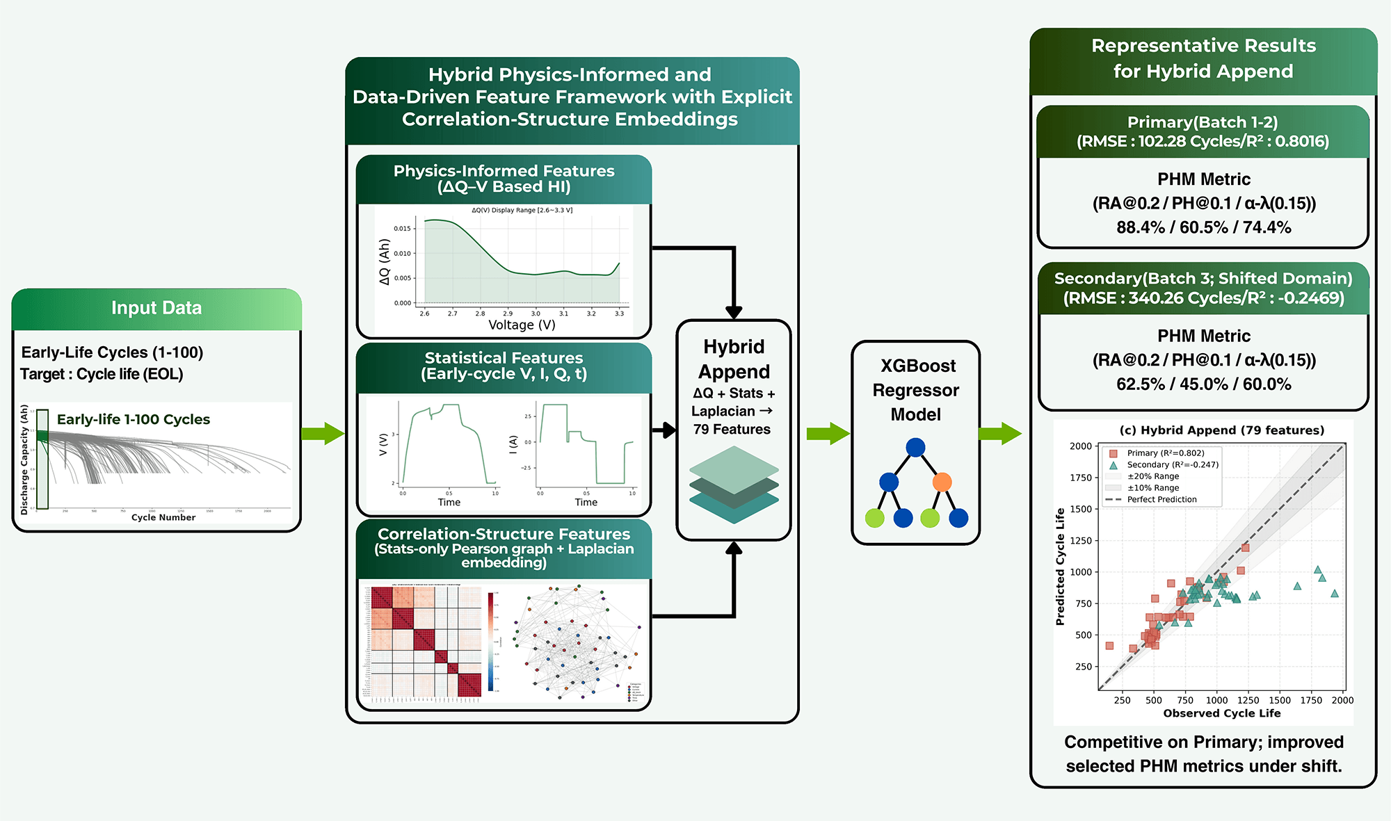
Early-life cycle-life prediction for lithium-ion batteries—estimating end-of-life from initial cycles—is valuable for rapid cell screening and battery health management. We investigate whether an explicit correlation-structure descriptor can complement physics-informed ΔQ-based indicators and generic early-cycle statistical features on the Severson 124-cell benchmark. We develop a lightweight hybrid framework that combines ΔQ-based health indicators, data-driven statistical features, and Laplacian Eigenmaps embeddings derived from a Pearson-correlation feature graph, with XGBoost used as the predictor. Across five feature configurations (ΔQ Only, ΔQ + Statistics, Hybrid Append, VIF + Laplacian, and Integrated Laplacian), we evaluate pointwise regression accuracy using RMSE and R2 together with PHM-style error-band measures RA@0.2, PH@0.1, and α-λ(0.15), computed on implied RUL trajectories induced by the early-life cycle-life estimate. On the Primary test domain, all four non-baseline configurations improved over ΔQ Only; Integrated Laplacian achieved the strongest RMSE/R2 pair (97.00 cycles, 0.8215), while Hybrid Append remained competitive (102.28 cycles, 0.8016) and improved RA@0.2 and PH@0.1 relative to ΔQ + Statistics. On the shifted Secondary domain, ΔQ Only gave the most favorable RMSE/R2 pair (267.82 cycles, 0.2275), whereas Hybrid Append and VIF + Laplacian improved selected error-band metrics. In an additional comparison against PCA, Random Projection, and Truncated SVD conducted at a matched 79-feature scale, with all transforms estimated from the training cells only, the graph-derived embedding remained competitive, but its margin over simpler reductions varied across splits. Taken together, these results support Hybrid Append as the main appended-structure configuration in this study, while indicating that the benefit of the correlation-structure descriptor is more visible in selected PHM-style error-band metrics than in uniformly improved pointwise accuracy.Graphic Abstract
Keywords
Lithium-ion batteries are widely deployed in electric vehicles, stationary energy-storage systems, aerospace, and defense applications. As adoption expands, prognostics and health management (PHM)—including remaining useful life (RUL) prediction—becomes increasingly important for safety, warranty planning, and operational efficiency. Recent reviews emphasize that practical battery PHM algorithms must balance predictive reliability with interpretability and deployment constraints such as limited data and changing operating conditions [1,2].
Within this landscape, early-life prediction aims to estimate the total cycle life of a cell using only a small fraction of the initial cycling data (e.g., the first 5%–10% of life). This capability is valuable for cell screening, quality control, and rapid iteration of cell design and fast-charging protocols [3–6]. However, it is inherently challenging because early degradation signatures are subtle, and available laboratory datasets are often small. Consequently, robustness and interpretability are as important as raw predictive accuracy.
Prior work on early-life prognostics spans three complementary directions. Physics-informed machine learning (PIML) embeds electrochemical knowledge and degradation constraints into learning pipelines to improve physical consistency [7–10]. Data-driven early-life methods leverage engineered early-cycle features or learned representations to predict cycle life from initial measurements [3–6]. Graph-based learning has also been explored to capture dependencies among signals, cells, or features, often through deep graph architectures [11–15]. While these approaches have advanced the field, practical gaps remain in small-sample early-life settings. High-capacity PIML and deep graph models can be difficult to tune and interpret when data are limited [1], and in many graph-deep-learning frameworks, the graph structure is implicit within the network, limiting direct inspection of which correlations drive predictions [11–15]. Moreover, feature choices should align with the intended deployment objective, since protocol-encoding features may inflate apparent accuracy while reducing transferability [16].
Beyond these methodological considerations, a further gap concerns evaluation. Many battery life-prediction studies report only static regression metrics such as RMSE or R2, which summarize pointwise error but say little about whether the implied RUL trajectory from an early-life cycle-life estimate stays within practically relevant error bands over time. In PHM, RUL is often assessed through trajectory-oriented measures—Relative Accuracy (RA), Prognostic Horizon (PH), and α-λ—that quantify error-band agreement and temporal consistency [17,18]. These metrics remain less common in early-life battery benchmarks that primarily emphasize RMSE/R2 [3–6]. Accordingly, we predict total cycle life from initial cycles and additionally evaluate the implied RUL trajectory using PHM-style error-band metrics.
Motivated by these gaps, we propose a lightweight early-life prognostics framework that emphasizes explicit structural representation together with PHM-style evaluation under both in-domain and shifted-domain settings. We use a fixed feature-correlation graph as an external structural descriptor and express it through Laplacian Eigenmaps alongside physics-informed ΔQ indicators in a small-sample early-life setting.
Our framework combines three feature groups: ΔQ-based health indicators as a physics-informed channel [3], generic early-cycle statistical features, and graph-derived structural embeddings obtained through Laplacian Eigenmaps on a Pearson-correlation feature graph [19,20]. XGBoost [21] is used as the predictor because it remains robust and parameter-efficient for tabular data in small-sample regimes.
Across five feature configurations (ΔQ Only, ΔQ + Statistics, Hybrid Append, VIF + Laplacian, and Integrated Laplacian), we evaluate both regression metrics (RMSE, R2) and PHM-style error-band metrics under an in-domain Primary split and a batch-shifted Secondary split. The analysis emphasizes graph construction confined to the training cells, comparisons performed at matched feature dimensionality, and the contrast between pointwise regression error and threshold-based PHM agreement.
This paper makes three contributions. First, we study a hybrid early-life prognostics pipeline that combines physics-informed ΔQ indicators, generic statistical features, and a fixed spectral descriptor derived from a feature-correlation graph. Second, we provide a stepwise feature-design workflow that keeps the physics-informed ΔQ channel explicit and separate from the correlation-structure descriptor at the feature-construction level. Third, we evaluate the resulting feature configurations using both standard regression metrics and PHM-style error-band metrics under a within-benchmark batch-shift setting in the Severson benchmark.
The remainder of this paper is organized as follows. Section 2 reviews related work on early-life prediction, physics-informed and graph-based learning, and PHM trajectory metrics. Section 3 describes the proposed hybrid feature pipeline and experimental protocol. Section 4 presents results using both regression and PHM metrics. Section 5 concludes with limitations and directions for future research.
This section reviews prior work most relevant to our study and clarifies how our approach is positioned. We focus on battery PHM and early-life cycle-life prediction, physics-informed and graph-based learning with an emphasis on interpretability and small-sample practicality, and PHM trajectory metrics for evaluating prognostic stability. The goal is to connect these threads to our design choice of using graph theory as an explicit, external feature-structure representation in a small-sample early-life setting.
2.1 Battery PHM and Early-Life Cycle-Life Prediction
Battery PHM spans degradation-mechanism understanding, state-of-health (SoH) estimation, RUL prediction, and decision-making for maintenance and operation across the battery life cycle. Comprehensive reviews summarize degradation modes, operational factors, and modeling paradigms and emphasize that interpretability and reliability are central to real-world PHM adoption [1].
Early-life prediction targets rapid life estimation using only initial cycles to enable screening and early decisions [3–6]. Severson et al. [3] established a widely used benchmark by showing that early-cycle voltage-curve-derived features (notably ΔQ−V) can be predictive of cycle life before substantial capacity fade. Subsequent studies explored alternative representations and learning models, including image-based encodings with CNNs [4,6], probabilistic regressors such as GPR with degradation-pattern recognition [5], and graphical feature constructions based on ΔQ−V IC/ΔQ curves [22]. Broader-condition work further examined early-life prediction under varying usage conditions and proposed degradation-informed or hierarchical approaches to improve extrapolation [23], while cross-condition deep learning frameworks such as BatLiNet aim to improve reliability across diverse ageing conditions via inter-cell learning mechanisms [24].
These efforts demonstrate the potential of early-cycle data while also highlighting practical trade-offs in small datasets: higher-capacity end-to-end models can be less transparent and more sensitive to modeling choices. In addition, recent perspective work emphasizes that feature selection should match the deployment objective, because protocol-encoding features can bias apparent performance and complicate transferability [16]. Our work adopts a pragmatic stance by combining physics-informed ΔQ indicators with generic statistics and an explicit correlation-structure representation to study whether a lightweight tabular pipeline can remain competitive without introducing a complex end-to-end graph learner.
Recent adjacent literature has also explored graph-based battery health modeling and alternative health metrics under related but non-identical tasks, including graph-based SOH estimation from partial discharge segments [25], alternative battery-health metrics such as Health EquiMetrics [26], and matrix-profile-based online knee-onset identification for lithium-ion battery SOH estimation [27]. Because many recent SOH-oriented and alternative battery-health studies use different prediction targets, sensing windows, and evaluation protocols, we discuss them as methodological context rather than as direct numerical baselines for the early-life cycle-life regression task considered here.
2.2 Physics-Informed and Graph-Based Learning: Expressiveness vs. Interpretability
Physics-informed machine learning (PIML) integrates physical constraints, electrochemical knowledge, or equivalent-circuit insights into learning pipelines, for example, by embedding governing equations into model structures or training objectives [7–10]. PIML can offer improved physical consistency and may enhance generalization when adequate domain information and data support are available. However, PIML often introduces additional modeling layers and expanded hyperparameter spaces, which can be burdensome in small-sample regimes and less accessible for practitioners without deep modeling expertise [1].
Graph-based learning has also received substantial attention for capturing structured dependencies among sensors, cells, or features. Recent approaches include spatio-temporal models with dynamic graphs [11], correlation- or attention-based GNN variants [12–14], and graph-attention–recurrent hybrids supported by explainable feature fragments [15]. These models can be powerful, but many treat the graph as an internal latent structure whose influence is not always straightforward to interpret directly; moreover, implicit graph learning can raise concerns about tuning effort and reproducibility in small datasets.
In contrast, our study should be understood as a graph-assisted feature-engineering case study. We use graph theory to construct a structurally explicit descriptor at the feature-correlation level. Specifically, we build a feature-by-feature correlation graph using Pearson coefficients [19] and compute low-dimensional Laplacian Eigenmaps embeddings [20] as compact representations of correlation structure. The contribution, therefore, lies in explicit spectral feature engineering rather than in a novel graph-learning architecture.
2.3 PHM Performance Metrics and Evaluation in Small-Sample Settings
Most battery life-prediction studies report static regression metrics such as RMSE, MAE, or R2. While these metrics quantify pointwise accuracy, they do not describe whether the RUL trajectory implied by a predicted cycle life remains inside practically relevant error bands over time. In PHM, RUL is often evaluated as a trajectory, motivating measures that summarize error-band agreement and temporal consistency rather than final pointwise error alone [17,18].
Saxena et al. [17] formalized offline prognostic metrics including RA, PH, and α-λ. RA measures the fraction of predictions within a specified tolerance band; PH summarizes how early predictions enter a tighter band; and α-λ captures agreement within a chosen tolerance window. Sharp [18] further discussed how such measures can be communicated to users with varied backgrounds. Despite their relevance, these trajectory-oriented metrics are still not routinely used in early-life battery benchmarks, where RMSE/R2 remain the dominant reporting metrics [3–6]. In this work, we therefore report both regression metrics and PHM-style error-band metrics computed on the implied RUL trajectories induced by each model’s early-life cycle-life estimate.
Accordingly, our work evaluates models using both regression metrics and PHM-style threshold-based accuracy measures, providing a complementary view of pointwise prediction quality and error-band agreement under batch shift.
We describe the problem formulation, the hybrid feature-engineering pipeline, the five feature-set configurations, and the XGBoost [21] modeling and evaluation protocol. The overall workflow is summarized in Fig. 1.

Figure 1: Overall pipeline of the proposed early-life cycle-life prediction framework. Early-life signals from the Severson 124-cell dataset are transformed into physics-informed ΔQ−V health indicators (HIs), data-driven statistical features, and Laplacian features (graph-based Laplacian features; Laplacian Eigenmaps projections) derived from a Pearson-correlation graph constructed on statistical features only. The resulting feature sets are used to train an XGBoost regressor with Bayesian hyperparameter optimization, and model performance is evaluated using RMSE, R2, and PHM-oriented metrics (RA@0.2, PH@0.1, α-λ(0.15)).
3.1 Dataset and Problem Formulation
We use the open Severson benchmark [3], which contains 124 commercial A123 APR18650M1A LFP/graphite cells cycled at 30°C under 72 one-step and two-step fast-charging policies. Cycle life is defined as the number of cycles until the cell reaches 80% of nominal capacity [3]. For each cell, the dataset provides cycle-resolved current, terminal voltage, charge/discharge capacity, time, temperature, and internal-resistance-related measurements.
Following Severson et al. [3], we formulate early-life cycle-life prediction as a supervised regression problem. For each cell, we use early-life cycles 1–100 as inputs and predict the total cycle life as the target.
For our evaluation, the dataset is organized into three batches (Batch 1–3). Batches 1–2 form the main development domain and are split into Train (41 cells; odd-indexed cells) and Primary Test (43 cells; even-indexed cells), whereas Batch 3 (40 cells) is retained as the Secondary Test set. Across all three batches, the common protocol backbone is fast charging from 0% to 80% SOC under one of the benchmark charging policies, an internal-resistance measurement at 80% SOC, a uniform 1C CC-CV top-off from 80% to 100% SOC to 3.6 V, and identical 4C CC-CV discharge to 2.0 V [3].
The batches nevertheless differ in their exact rest schedules and in the placement of short pauses around the 80% SOC/internal-resistance/discharge steps. Severson et al. report 1 min and 1 s rests after reaching 80% SOC and after discharge, respectively, for the 12 May 2017 batch; 5 min rests at both locations for the 30 June 2017 batch; and 5 s rests after reaching 80% SOC, after the internal-resistance test, and both before and after discharge for the 12 April 2018 batch [3]. Together, these protocol and distributional differences motivate treating Batch 3 as a protocol-shifted secondary evaluation domain rather than as an in-domain test split. The batch-specific rest/pause schedules and their roles in the evaluation are summarized in Table 1.

Because several point features are computed from current, time, and capacity trajectories over cycles 1–100, differences in rest timing and pause placement can directly alter the empirical distribution of the statistical-feature channel even when the underlying chemistry is unchanged.
After feature extraction, each cell is represented as a single tabular feature vector. Early-life time series are summarized into physics-informed indicators, generic statistics, and correlation-structure descriptors, yielding a regression task suitable for tree-based gradient boosting.
3.2 Hybrid Feature Engineering
Our feature engineering comprises three groups: (i) physics-informed ΔQ−V health indicators, (ii) data-driven statistical features, and (iii) Laplacian features that encode correlation structure among the statistical features.
3.2.1 Physics-Informed ΔQ−V Health Indicators
We build on the ΔQ-based health indicators introduced by Severson et al. [3]. Using early-life charging curves (cycles 10–100), we align capacity-voltage curves onto a common voltage grid and compute ΔQ between selected cycle pairs within voltage bins, producing ΔQ signatures. We then summarize these signatures into seven scalar HIs that capture the magnitude, variability, and characteristic shifts of ΔQ along the voltage axis, including statistics computed over degradation-sensitive voltage regions.
These seven HIs are treated as physics-informed descriptors because they arise from physically motivated signal transforms that have previously shown relevance to cycle-life variability in early-life prediction settings [3]. Here, they serve as a dedicated physics-informed feature channel rather than as direct mechanistic state variables.
3.2.2 Data-Driven Point Features
The second feature group consists of generic statistical features computed directly from early-cycle signals without using ΔQ transforms. Here, Qdlin denotes the linearly interpolated discharge-capacity signal represented on a common voltage grid. From cycles 1–100, we extract 52 statistical features organized into five families: current-derived, time-derived, capacity-derived, differential-capacity–derived, and interaction-derived features. Across these families, the features are generated by applying four summary operators—mean, standard deviation, minimum, and maximum—to raw, transformed, ratio, and interaction signals. A compact family-wise summary is provided in Table 2, and Table A1 in Appendix A lists the complete grouped set of the 52 feature names.

These statistical features complement the ΔQ health indicators by capturing broader early-cycle distributional characteristics and transformed-signal patterns present in the raw measurements.
3.2.3 Correlation Graph and Laplacian Features
The third feature group uses an explicit graph-theoretic representation to encode correlation structure among the 52 statistical features. To avoid information leakage, the correlation graph is constructed using the training cells only (41 cells).
Let
Visualization (Fig. 2). For visualization, we display

Figure 2: Correlation structure of the statistical feature set computed from the training cells. (a) Pearson correlation heatmap of the 52 statistical features. (b) Correlation network visualization with edges shown for |r| > 0.3, where nodes represent features and node colors indicate feature categories.
Graph construction. For the actual Laplacian feature generation, we define a weighted graph over features using off-diagonal absolute Pearson correlations while excluding self-correlations. Specifically,
Laplacian Eigenmaps. We apply Laplacian Eigenmaps [20] and extract

Figure 3: Two-dimensional Laplacian Eigenmaps embedding of the 52 statistical-feature nodes constructed from the correlation graph in Fig. 2. Features with similar correlation profiles form clusters; colors denote feature categories.
Cell-level Laplacian features. Laplacian Eigenmaps provides coordinates for feature nodes. To obtain cell-level features for XGBoost, we project each cell’s standardized statistical feature vector onto the selected eigenvector subspace. Before projection, statistical features are z-scored using the training-set mean and standard deviation, and the same transformation is applied to the Primary and Secondary test sets. Let
and use
Figs. 2 and 3 are presented as structural diagnostics of the statistical-feature space, not as direct explanations of predictor behavior. Accordingly, the present study interprets the graph component at the level of feature-space organization rather than feature-attribution to individual predictions.
We evaluated k over a prespecified candidate set and found broadly similar behavior across mid-range embedding dimensions, although the best observed value differed by metric and split. We therefore retain k = 20 as a practical mid-range operating dimension. The quantitative sensitivity results obtained with graph construction confined to the training cells are shown in Fig. A1 in Appendix B: over the explored grid, the best observed values occurred at k = 5 for CV R2, k = 25 for Primary R2, and k = 15 for Secondary R2. Importantly, ΔQ−V HIs are not included in the correlation graph: the graph is built on the statistical features only, and ΔQ−V HIs remain an independent physics-informed channel. The Integrated Laplacian variant, which recomputes the graph after adding ΔQ−V HIs, is retained as an explicit ablation in the experiments. Table 3 summarizes the three feature groups.

3.3 Feature-Set Design and XGBoost Modeling
Using the three feature groups above, we define five feature configurations to isolate the incremental value of adding statistics and correlation structure on top of the ΔQ−V baseline.
• ΔQ Only. ΔQ−V HI (7) only. This is closest to the Severson-style ΔQ−V baseline and serves as a physics-informed reference.
• ΔQ + Statistics. ΔQ−V HI (7) plus Stats (52), totaling 59 features. This tests whether generic statistics add complementary information beyond ΔQ−V.
• Hybrid Append. ΔQ−V HI (7) plus Stats (52) plus Laplacian (20), totaling 79 features. This is the main proposed configuration.
• VIF + Laplacian. A compact variant in which multicollinear statistical features are pruned using Variance Inflation Factor (VIF), and the remaining statistics are combined with Laplacian (20), totaling 47 features.
• Integrated Laplacian. A comparison setting in which ΔQ−V HI and Stats are jointly used to recompute the correlation graph and Laplacian, producing 99 features. This contrasts with Hybrid Append, where ΔQ−V remains a separate channel.
Regression model. We use XGBoost [21] for all feature sets. XGBoost is well-suited to tabular data, captures non-linear interactions, and is relatively parameter-efficient in small-sample regimes. Because tree-based models tolerate heterogeneous feature scales, we combine ΔQ−V HI, Stats, and Laplacian features without requiring additional normalization for the regressor.
Training and hyperparameter tuning. To enable fair comparison across feature sets, we use a common training protocol. We perform 5-fold cross-validation on the 41 training cells. Key hyperparameters (e.g., tree depth, learning rate, number of estimators, min_child_weight, subsample, colsample_bytree, and λ regularization) are optimized using Optuna-based hyperparameter optimization, with cross-validation RMSE as the objective. The final model is retrained on the full training set using the selected hyperparameters and evaluated on the Primary and Secondary test sets. All scalers, correlation graphs, Laplacian bases, and PCA/RP/TSVD transforms were fit on the training cells only and then applied unchanged to the Primary and Secondary test splits.
Table 4 summarizes the feature-set configurations.

3.4 Evaluation Metrics and PHM-Oriented Assessment
We evaluate each feature configuration using both standard regression metrics and PHM-oriented error-band metrics.
Regression metrics. We report RMSE and R2 for pointwise cycle-life prediction accuracy.
PHM-style error-band metrics. In addition to RMSE and R2, we assess PHM-style behavior using trajectory-oriented metrics [17,18]. For each cell, the model outputs a single early-life estimate of total cycle life. From this estimate we construct an implied RUL trajectory by subtracting the cycle index t from the predicted cycle life, while the true RUL is obtained by subtracting t from the observed cycle life. Because the model does not generate sequentially updated predictions, these metrics are applied to the implied trajectory induced by the fixed early-life estimate. We then compute relative error along the trajectory and report:
• RA@0.2: the fraction of time points where the relative error is within ±20%;
• PH@0.1: a stricter error-band agreement measure based on a ±10% error tolerance;
• α-λ(0.15): a summary score capturing where the relative error remains within a ±15% band.
We report RMSE, R2, and the three PHM metrics for both the Primary and Secondary test sets. This dual evaluation complements pointwise regression accuracy by adding an error-band view of performance under domain shift.
We present quantitative results for the five feature configurations defined in Section 3.3 under the common training and evaluation protocol. The section first summarizes cross-validation on the Train set, then reports held-out performance on the Primary and Secondary test domains, and finally examines whether the Hybrid Append gain can be reproduced by simpler reduced-dimensional baselines.
4.1 Role of Cross-Validation in Model Selection
Cross-validation on the 41-cell training set was used for model selection and hyperparameter tuning. In this small-sample setting, richer feature configurations often appeared promising in CV, but the held-out ordering changed across the Primary and Secondary domains.
Accordingly, the main scientific interpretation in this section is anchored in the held-out test results and the accompanying bootstrap intervals. The additional matched-dimensionality comparisons and the k-sensitivity analysis then provide comparative and robustness evidence for the graph-derived descriptor.
4.2 Held-out Test Performance on the Primary and Secondary Domains
Tables 5 and 6 report the held-out test results for the five feature configurations. Taken together, they highlight the contrast between in-domain performance on Batches 1–2 and shifted-domain generalization on Batch 3. The split difference is substantial not only protocol-wise (Section 3.1) but also distributionally: the Primary split has median cycle life 520 cycles, whereas the Secondary split has median 964.5 cycles. The bootstrap intervals reported in Tables 5 and 6 quantify uncertainty for RMSE and R2 only; RA, PH, and α-λ are reported as point estimates.


4.2.1 Primary Test Set (Batch 1–2)
Table 5 shows that on the Primary test split, all augmented feature configurations improved over ΔQ Only. No single method dominated every metric. Integrated Laplacian achieved the lowest RMSE and highest R2 (97.00 cycles, 0.8215; 95% bootstrap CIs: [71.87, 120.22] and [0.6519, 0.8970]), while Hybrid Append remained competitive in pointwise error (102.28 cycles, 0.8016; [71.87, 128.95] and [0.6035, 0.8969]) and delivered one of the stronger PHM-style profiles (RA@0.2/PH@0.1/α-λ(0.15) = 88.4/60.5/74.4). Relative to ΔQ + Statistics, Hybrid Append preserved very similar RMSE/R2 while improving RA@0.2 and PH@0.1, suggesting that the appended structural channel was more visible in PHM-style error-band metrics than in pointwise error alone. Although the Integrated Laplacian achieved the strongest Primary RMSE/R2 pair, the Hybrid Append design remains important because it preserves the explicit ΔQ branch while adding a competitive structural descriptor. In this sense, the Primary split supports Hybrid Append as a practically well-balanced appended design rather than as a uniformly dominant configuration.
4.2.2 Secondary Test Set (Batch 3, Domain Shift)
Table 6 shows that on the Secondary test split, ΔQ only gave the most favorable RMSE/R2 pair among the tested configurations, with RMSE/R2 of 267.82/0.2275 (95% bootstrap CIs: [194.18, 338.27] and [−0.1015, 0.3851]). VIF + Laplacian was the next most competitive shifted-domain configuration in R2 (0.1662) and achieved the highest RA@0.2 (70.0). Hybrid Append improved over ΔQ + Statistics and Integrated Laplacian in both RMSE and R2 and reached the highest PH@0.1 (45.0), but it did not exceed ΔQ Only on RMSE or R2. Under the shifted Batch 3 domain, the sparse ΔQ-only baseline remained the most robust pointwise regressor, whereas Hybrid Append and VIF + Laplacian improved selected PHM threshold metrics. This contrast is informative for the proposed design: while the strongest shifted-domain RMSE/R2 remained with the sparse physics-informed baseline, Hybrid Append retained value as the study’s principal hybrid configuration by preserving the explicit ΔQ channel and improving selected error-band metrics under shift.
The integrated-graph ablation is also revealing: although Integrated Laplacian was strong on the Primary split, it generalized poorly to Batch 3, which favors keeping ΔQ as a separate physics-informed branch rather than absorbing it into the graph.
4.3 Comparison against Simpler Reduced-Dimensional Baselines
To examine whether the Hybrid Append behavior could be reproduced by generic dimensionality reduction alone, we conducted an additional comparison against three non-graph alternatives at a matched 79-feature scale. These alternatives were obtained by appending 20 features from PCA, Gaussian Random Projection, and Truncated SVD to the 59-feature ΔQ + Statistics baseline, as shown in Fig. 4. This supplementary analysis helps interpret the appended structural descriptor alongside the main five-configuration held-out results.

Figure 4: Comparison at a matched 79-feature scale against simpler reduced-dimensional baselines. Primary and Secondary test R2 are shown for ΔQ + Statistics (59 features), Hybrid Append (79 features), and three 79-feature alternatives obtained by appending 20 features from PCA, Random Projection, and Truncated SVD. All learned transforms were estimated from the training cells only.
All compared variants were evaluated under a common train/Primary/Secondary split and XGBoost protocol, and every learned transform was fit on the training cells only before being applied unchanged to the Primary and Secondary test splits.
In this comparison, with all learned transforms estimated from the training cells and then applied unchanged to the test splits, Hybrid Append achieved CV R2 0.7497, Primary R2 0.8185, and Secondary R2 −0.3205. The best matched-dimensionality non-graph baseline reached Primary R2 0.8107 and Secondary R2 −0.1955, while +RandomProjection20 achieved the highest CV R2. The comparison is therefore mixed rather than uniform: the graph-derived embedding remained competitive, but its margin over simpler reductions at the same feature dimensionality depended on the evaluation split. These results instead position Hybrid Append as the study’s principal hybrid configuration, whose added value is best understood as complementary and split-dependent.
4.4 PHM-Oriented Analysis of Implied RUL Trajectories
Fig. 5 compares RA@0.2, PH@0.1, and α-λ (0.15) across feature sets on both test domains. These PHM-style error-band metrics highlight differences that are not fully captured by RMSE and R2 alone. For compact visualization, Fig. 5 displays the scores on a 0–1 scale, whereas Tables 5 and 6 report the corresponding values in percentage form. Because each model produces a single early-life cycle-life estimate per cell, the scores are computed on the implied RUL trajectory defined in Section 3.4.

Figure 5: PHM-oriented error-band metrics on the implied RUL trajectories for the Primary and Secondary test sets: (a) RA@0.2 (±20% tolerance), (b) PH@0.1 (±10% tolerance), and (c) α-λ (0.15) (±15% tolerance) for ΔQ Only, ΔQ + Statistics, Hybrid Append, VIF + Laplacian, and Integrated Laplacian. Scores are shown as proportions on a 0–1 scale; the dashed line indicates the ideal score (1.0).
On the Primary split, Hybrid Append and Integrated Laplacian tie for the highest RA@0.2 (88.4%), Hybrid Append and VIF + Laplacian tie for the highest PH@0.1 (60.5%), and VIF + Laplacian achieves the highest α-λ(0.15) (76.7%). On the Secondary split, VIF + Laplacian reaches the highest RA@0.2 (70.0), Hybrid Append reaches the highest PH@0.1 (45.0), and ΔQ + Statistics, Hybrid Append, and VIF + Laplacian tie on α-λ(0.15) (60.0).
Viewed together with the held-out RMSE/R2 results, the PHM-style metrics suggest that the contribution of the appended structural channel is not expressed identically across evaluation criteria. Thus, no single configuration dominates across all criteria; instead, the preferred feature set depends on whether the emphasis is on pointwise regression error or stricter error-band agreement. In particular, the Hybrid Append configuration is most naturally interpreted as improving selected error-band behavior while maintaining competitive pointwise accuracy on the in-domain split and improving PH@0.1 relative to ΔQ + Statistics on both test domains (60.5 vs. 55.8 on Primary; 45.0 vs. 42.5 on Secondary).
4.5 Visualization of Prediction Distributions
To complement the aggregate metrics, Fig. 6 plots observed vs. predicted cycle life for the Primary and Secondary test cells across the five feature configurations. The Primary-domain points cluster much closer to the identity line than the Secondary points, consistent with the protocol differences summarized in Table 1 and the shifted-domain performance reported in Table 6.

Figure 6: Observed vs. predicted cycle life for the five feature configurations: (a) ΔQ Only, (b) ΔQ + Statistics, (c) Hybrid Append, (d) VIF + Laplacian, and (e) Integrated Laplacian. Red squares and green triangles denote Primary Test and Secondary Test cells, respectively. The dashed line indicates perfect prediction, and shaded bands represent ±10% and ±20% relative-error regions.
Among the augmented feature sets, the Primary scatter for ΔQ + Statistics, Hybrid Append, and Integrated Laplacian is comparatively tight, consistent with the stronger in-domain RMSE/R2 values in Table 5. The broader Secondary dispersion of the integrated variant mirrors its weaker shifted-domain behavior, while Hybrid Append remains visually close to ΔQ + Statistics in pointwise scatter but achieves slightly stronger PH@0.1. Viewed together with Tables 5 and 6 and Fig. 5, these plots indicate that added feature channels help in-domain, whereas shifted-domain behavior remains more metric-dependent.
This paper examined early-life cycle-life prediction for lithium-ion batteries in a small-sample setting, focusing on whether an explicit correlation-structure descriptor can complement physics-informed ΔQ indicators and generic early-cycle statistical features. The graph component was implemented as a fixed spectral feature-engineering step derived from a feature-correlation graph.
Across the five main feature configurations, all augmented feature sets improved over ΔQ Only on the in-domain Primary split, but no single configuration dominated every metric. Integrated Laplacian achieved the strongest Primary RMSE/R2 pair, whereas Hybrid Append remained competitive in pointwise accuracy and delivered one of the stronger PHM-style profiles. Relative to ΔQ + Statistics, Hybrid Append preserved similar Primary RMSE/R2 while improving RA@0.2 and PH@0.1, which highlights the practical value of the appended structural channel.
Under the shifted Batch 3 domain, the sparse ΔQ-only baseline remained the most robust pointwise regressor, while Hybrid Append and VIF + Laplacian improved selected PHM threshold metrics. Taken together, these findings support Hybrid Append as the study’s principal hybrid configuration: it preserves the explicit ΔQ branch, remains competitive on the Primary split, and provides a more favorable appended design than the integrated-graph alternative when error-band behavior under shift is also considered.
The additional comparison at a matched 79-feature scale against PCA, Random Projection, and Truncated SVD further refines this interpretation. In those comparisons, all learned transforms were estimated from the training cells and then applied unchanged to the test splits. The graph-derived embedding remained competitive, but its margin over simpler reductions varied by split. The graph component is therefore best understood not as a universal substitute for generic dimensionality reduction, but as a complementary structural descriptor within the Hybrid Append design.
Overall, this work contributes (i) a small-sample case study of combining physics-informed indicators, generic statistical features, and graph-derived structural descriptors for early-life battery prognostics, (ii) a feature-design workflow that keeps the ΔQ channel explicit while adding an explicit correlation-structure descriptor, and (iii) a joint evaluation using regression and PHM-style error-band metrics under a within-benchmark batch-shift setting. In practical terms, the present evidence supports using the appended correlation-structure descriptor as a supplementary design option when PHM-style tolerance behavior is of interest, while pointwise shifted-domain accuracy should still be benchmarked against sparse physics-informed baselines.
This work also has limitations. Experiments were conducted on a single public benchmark (the Severson 124-cell LFP/graphite dataset) with a specific early-life window (cycles 1–100) and a batch-defined domain shift. Both the structural descriptor and the PHM-style evaluation remain intentionally simple at this stage: the graph descriptor is based on Pearson correlation, and the PHM-style metrics are computed from the implied RUL trajectory induced by a single early-life estimate per cell rather than from sequentially updated online predictions. The present results therefore establish within-benchmark behavior for this early-life setting.
Future work will extend the framework in several directions. First, we will evaluate robustness across additional chemistries, protocols, and datasets. Second, we will investigate alternative correlation-structure constructions, such as sparsified graphs, partial-correlation, or regularized dependence measures, to improve structural stability under protocol changes. Third, we will incorporate uncertainty-aware prediction and assess PHM performance with explicit uncertainty quantification. Finally, we will examine model-selection and evaluation strategies for sequential or online prediction settings while maintaining interpretability and small-sample practicality.
Acknowledgement: None.
Funding Statement: This research was funded by the National Research Foundation of Korea (NRF) grant funded by the Korea government (MSIT) (No. NRF-2022R1C1C1011743).
Author Contributions: The authors confirm contribution to the paper as follows: study conception and design: Kang-Woo Lee; data collection: Kang-Woo Lee; analysis and interpretation of results: Kang-Woo Lee; draft manuscript preparation: Kang-Woo Lee; supervision and manuscript review: Dong-Hee Lee and Dae-Il Kwon. All authors reviewed and approved the final version of the manuscript.
Availability of Data and Materials: The data supporting the findings of this study are publicly available from the Severson lithium-ion battery dataset at https://data.matr.io/1/.
Ethics Approval: Not applicable.
Conflicts of Interest: The authors declare no conflicts of interest.
Appendix A

Appendix B

Figure A1: Train-only sensitivity analysis of the Laplacian embedding dimension k. CV, primary, and secondary performance are shown across multiple values of k using R2 (left) and RMSE (right). Mid-range values perform comparably, but the best observed values differ by metric and split; k = 20 is therefore presented as a practical mid-range operating point rather than as a unique optimum.
References
1. Che Y, Hu X, Lin X, Guo J, Teodorescu R. Health prognostics for lithium-ion batteries: mechanisms, methods, and prospects. Energy Environ Sci. 2023;16(2):338–71. doi:10.1039/d2ee03019e. [Google Scholar] [CrossRef]
2. Thelen A, Huan X, Paulson N, Onori S, Hu Z, Hu C. Probabilistic machine learning for battery health diagnostics and prognostics—review and perspectives. npj Mater Sustain. 2024;2(1):14. doi:10.1038/s44296-024-00011-1. [Google Scholar] [CrossRef]
3. Severson KA, Attia PM, Jin N, Perkins N, Jiang B, Yang Z, et al. Data-driven prediction of battery cycle life before capacity degradation. Nat Energy. 2019;4(5):383–91. doi:10.1038/s41560-019-0356-8. [Google Scholar] [CrossRef]
4. Zhou S, Wang Q, Yang F. Early lifetime prediction of lithium-ion batteries based on classical image encoding methods. Energy. 2025;336(2):138372. doi:10.1016/j.energy.2025.138372. [Google Scholar] [CrossRef]
5. Fu L, Jiang B, Zhu J, Wei X, Dai H. Early remaining useful life prediction for lithium-ion batteries using a Gaussian process regression model based on degradation pattern recognition. Batteries. 2025;11(6):221. doi:10.3390/batteries11060221. [Google Scholar] [CrossRef]
6. Yang W, Yang H. Ultra-early prediction of lithium-ion battery cycle life based on assembled capacity curve extracted from a single cycle. J Power Sources. 2025;640(3):236620. doi:10.1016/j.jpowsour.2025.236620. [Google Scholar] [CrossRef]
7. Nascimento RG, Viana FAC, Corbetta M, Kulkarni CS. A framework for Li-ion battery prognosis based on hybrid Bayesian physics-informed neural networks. Sci Rep. 2023;13(1):13856. doi:10.1038/s41598-023-33018-0. [Google Scholar] [PubMed] [CrossRef]
8. Ma L, Tian J, Zhang T, Guo Q, Hu C. Accurate and efficient remaining useful life prediction of batteries enabled by physics-informed machine learning. J Energy Chem. 2024;91:512–21. doi:10.1016/j.jechem.2023.12.043. [Google Scholar] [CrossRef]
9. Shi J, Rivera A, Wu D. Battery health management using physics-informed machine learning: online degradation modeling and remaining useful life prediction. Mech Syst Signal Process. 2022;179(7):109347. doi:10.1016/j.ymssp.2022.109347. [Google Scholar] [CrossRef]
10. Wang F, Zhai Z, Zhao Z, Di Y, Chen X. Physics-informed neural network for lithium-ion battery degradation stable modeling and prognosis. Nat Commun. 2024;15(1):4332. doi:10.1038/s41467-024-48779-z. [Google Scholar] [PubMed] [CrossRef]
11. Chen Z, Qian Q. DGL-STFA: predicting lithium-ion battery health with dynamic graph learning and spatial-temporal fusion attention. Energy AI. 2025;19(7):100462. doi:10.1016/j.egyai.2024.100462. [Google Scholar] [CrossRef]
12. Wu W, Chen Z, Liu W, Pan E. Correlation based-graph neural network for health prognosis of non-fully charged and discharged lithium-ion batteries. J Power Sources. 2025;629(2):235984. doi:10.1016/j.jpowsour.2024.235984. [Google Scholar] [CrossRef]
13. Wei Y, Wu D. Prediction of state of health and remaining useful life of lithium-ion battery using graph convolutional network with dual attention mechanisms. Reliab Eng Syst Saf. 2023;230(1):108947. doi:10.1016/j.ress.2022.108947. [Google Scholar] [CrossRef]
14. Gu X, Liu M, Tian J. State of health estimation for batteries based on a dynamic graph pruning neural network with a self-attention mechanism. Energies. 2025;18(20):5333. doi:10.3390/en18205333. [Google Scholar] [CrossRef]
15. Luan W, Cai H, Wang X, Zhao B. State of health for lithium-ion batteries based on explainable feature fragments via graph attention network and bi-directional gated recurrent unit. Sensors. 2025;25(19):5953. doi:10.3390/s25195953. [Google Scholar] [PubMed] [CrossRef]
16. Geslin A, van Vlijmen B, Cui X, Bhargava A, Asinger PA, Braatz RD, et al. Selecting the appropriate features in battery lifetime predictions. Joule. 2023;7(9):1956–65. doi:10.1016/j.joule.2023.07.021. [Google Scholar] [CrossRef]
17. Saxena A, Celaya J, Saha B, Saha S, Goebel K. Metrics for offline evaluation of prognostic performance. Int J Progn Health Manag. 2010;1(1):4–23. doi:10.36001/ijphm.2010.v1i1.1336. [Google Scholar] [CrossRef]
18. Sharp ME. Simple metrics for evaluating and conveying prognostic model performance to users with varied backgrounds. Annu Conf PHM Soc. 2013;5(1):1–10. doi:10.36001/phmconf.2013.v5i1.2317. [Google Scholar] [CrossRef]
19. Lee Rodgers J, Nicewander WA. Thirteen ways to look at the correlation coefficient. Am Stat. 1988;42(1):59–66. doi:10.1080/00031305.1988.10475524. [Google Scholar] [CrossRef]
20. Belkin M, Niyogi P. Laplacian eigenmaps for dimensionality reduction and data representation. Neural Comput. 2003;15(6):1373–96. doi:10.1162/089976603321780317. [Google Scholar] [CrossRef]
21. Chen T, Guestrin C. Xgboost: a scalable tree boosting system. In: Proceedings of the 22nd ACM SIGKDD International Conference on Knowledge Discovery and Data Mining; 2016 Aug 13–17; San Francisco, CA, USA. p. 785–94. doi:10.1145/2939672.2939785. [Google Scholar] [CrossRef]
22. He N, Wang Q, Lu Z, Chai Y, Yang F. Early prediction of battery lifetime based on graphical features and convolutional neural networks. Appl Energy. 2024;353:122048. doi:10.1016/j.apenergy.2023.122048. [Google Scholar] [CrossRef]
23. Li T, Zhou Z, Thelen A, Howey DA, Hu C. Predicting battery lifetime under varying usage conditions from early aging data. Cell Rep Phys Sci. 2024;5(4):101891. doi:10.1016/j.xcrp.2024.101891. [Google Scholar] [CrossRef]
24. Zhang H, Li Y, Zheng S, Lu Z, Gui X, Xu W, et al. Battery lifetime prediction across diverse ageing conditions with inter-cell deep learning. Nat Mach Intell. 2025;7(2):270–7. doi:10.1038/s42256-024-00972-x. [Google Scholar] [CrossRef]
25. Zhou KQ, Qin Y, Yuen C. Graph neural network-based lithium-ion battery state of health estimation using partial discharging curve. J Energy Storage. 2024;100(11):113502. doi:10.1016/j.est.2024.113502. [Google Scholar] [CrossRef]
26. Zhou KQ, Qin Y, Bhattacharjee A, Tushar W, Chong ACC, Yuen C. Health EquiMetrics for battery assessment—a novel metric for end-of-life evaluation beyond state-of-health. J Energy Storage. 2026;147(2):120064. doi:10.1016/j.est.2025.120064. [Google Scholar] [CrossRef]
27. Zhou KQ, Qin Y, Yuen C. Lithium-ion battery state of health estimation by matrix profile empowered online knee onset identification. IEEE Trans Transp Electrif. 2024;10(1):1935–46. doi:10.1109/TTE.2023.3265981. [Google Scholar] [PubMed] [CrossRef]
Cite This Article
 Copyright © 2026 The Author(s). Published by Tech Science Press.
This work is licensed under a Creative Commons Attribution 4.0 International License , which permits unrestricted use, distribution, and reproduction in any medium, provided the original work is properly cited.
 Downloads
 Citation Tools