Structured Future Interpretation for Predictive and Explainable Autonomous Driving

1  Introduction

Autonomous driving systems are increasingly expected to satisfy two complementary requirements: reliable decision-making in dynamic environments and transparent justification of their actions [1,2]. Complementary work has explored hybrid LLM-based obstacle avoidance and VLM–LLM navigation in embedded robotics [3,4]. While recent advances in computer vision, multimodal learning, and temporal modeling have improved scene understanding and maneuver prediction, explainability remains limited under realistic deployment conditions. In safety-critical scenarios, it is insufficient for a system to output only an action such as stopping, turning, or changing lane; it should also explain why the action was selected, how confident the system is, and whether anticipated future risk influenced the decision.

A key limitation of many existing explainable driving approaches is that explanations are often generated from ground-truth annotations or current-state predictions alone. This creates a mismatch between training and deployment: during deployment, explanations must rely on imperfect upstream predictions, whereas many training pipelines condition explanations on idealized annotations. As a result, generated explanations may describe oracle behavior rather than the actual reasoning process of the deployed system [5].

A second limitation is the insufficient treatment of future scene evolution. Many approaches rely on frame-level perception or short temporal aggregation without explicitly modeling how risk evolves over the next few seconds. However, driving decisions are inherently future-dependent: a pedestrian may move toward a crosswalk, a vehicle may merge into the ego lane, or an initially safe trajectory may become unsafe due to a delayed obstacle [6,7]. In such cases, current-state explanations are incomplete because the reason for an action may lie in an anticipated future outcome rather than in the immediate observation.

Predictive world models offer a promising way to address this issue by forecasting future latent scene states from past observations and ego-motion signals [8,9]. However, prediction alone is not sufficient. A predicted trajectory must be converted into decision-relevant information, such as increasing risk, decreasing clearance, or time-to-critical events. Without this interpretation step, a decision module may still favor short-term progress even when the predicted future contains delayed hazards. This motivates the central question of this work:

How can predicted futures be transformed into structured representations that improve both decision-making and explanation generation under ambiguity?

To answer this question, we propose a predictive explainable driving framework centered on a lightweight Future Interpretation Module (FIM). The framework combines latent world modeling, structured perception, and language-based explanation generation. A transformer-based latent world model predicts action-conditioned future latent rollouts. The proposed FIM then converts these rollouts into structured future summaries, including risk trend, peak risk, time-to-critical, minimum clearance, predicted collision, dominant predicted event, and confidence. These summaries are used by the decision module to evaluate candidate actions and by the explanation module to generate temporally grounded justifications.

The proposed framework follows a modular pipeline. First, past observations and ego-motion signals are encoded into a latent state, from which a world model predicts action-conditioned future rollouts. Second, a multi-expert temporal perception model produces structured current predictions, including action, reasoning factors, confidence, and risk. Third, the FIM interprets predicted latent futures using the same structured representation, ensuring consistency between current and future reasoning. Fourth, a model-based decision module evaluates candidate actions using both progress and predicted future risk. Finally, a language explanation module generates natural language justifications conditioned on the selected action, current structured predictions, and future summaries.

To validate the proposed approach, we conduct both dataset-based evaluation and a controlled scenario-based experiment. In particular, we introduce an Ambiguous Future Risk Trade-off scenario in NVIDIA Isaac Sim, where the ego vehicle must choose between a short direct route that initially appears safe and a longer bypass that remains safer over time. A delayed dynamic obstacle creates ambiguity that cannot be resolved from the current observation alone. This experiment directly tests whether structured interpretation of predicted futures improves risk anticipation and action selection compared with a prediction-only baseline.

1.1 Training–Deployment Mismatch in Explainable Driving

A central difficulty in explainable autonomous driving is the mismatch between the information used to train an explanation model and the information available during deployment. Many explanation pipelines are trained using ground-truth actions, object annotations, semantic reasons, or future events. At deployment time, however, the explanation generator receives imperfect outputs from perception, prediction, and planning modules. Consequently, a fluent explanation may refer to an object that was not detected, justify an action different from the action actually selected, express excessive certainty, or describe an oracle future rather than the future predicted by the deployed system. Such explanations are not merely incomplete; they can be unfaithful to the actual decision process and may encourage inappropriate human trust.

The proposed framework reduces this mismatch by conditioning explanations on prediction-derived structured variables. The explanation input contains the selected action, semantic reasoning factors, confidence, current risk, the structured summary of the selected future rollout, and evidence associated with rejected alternatives. During training, controlled perturbations of these fields expose the language module to realistic upstream errors. The objective is therefore not to guarantee that every explanation is correct, but to make the explanation traceable to the same model-derived evidence that influenced the deployed decision.

1.2 Novelty Statement

The individual quantities used by FIM—including risk trend, peak risk, time-to-critical, minimum clearance, predicted collision, dominant predicted event, and confidence—are established concepts and are not claimed as novel in isolation. The contribution lies in their integration into a common interpretation interface between action-conditioned latent prediction and two downstream functions: safety-aware action selection and natural-language explanation. For every candidate action, the framework converts a latent future sequence into a compact summary that expresses temporal urgency, worst-case risk, safety margin, trend, confidence, and event semantics. This shared structured representation makes the predicted future inspectable, supports direct descriptor-level ablation, and provides an explicit connection between the variables used to choose an action and the variables used to explain it.

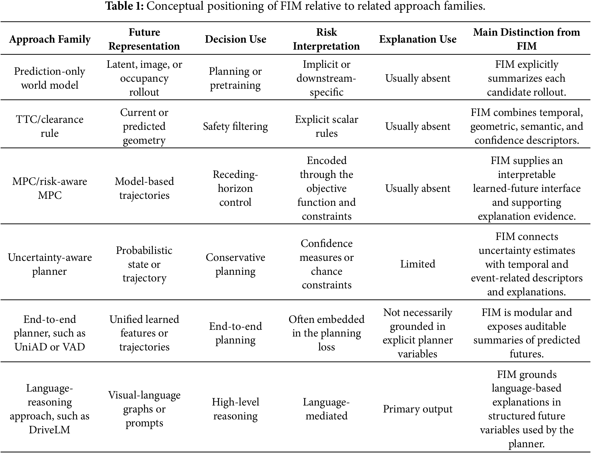
This positioning distinguishes the proposed method from prediction-only world models, current-state risk filters, generic MPC objectives, occupancy forecasting used only for planning, and explanation systems conditioned primarily on present observations or ideal annotations. FIM is intended as an interpretation layer that can complement—not replace—these planning and prediction paradigms.

1.3 Contributions

1.    An aligned prediction–interpretation–decision–explanation framework in which action-conditioned future latent states are mapped to the structured perception space through an explicitly trained alignment interface.

2.    A Future Interpretation Module that summarizes each candidate future using risk trend, peak risk, time-to-critical, minimum clearance, predicted collision, dominant predicted event, and confidence.

3.    A reproducible safety-aware decision rule that separates hard safety rejection from soft progress, risk, clearance, uncertainty, and route-commitment costs.

4.    A prediction-conditioned explanation formulation in which the selected action and rejected alternatives are explained from the same structured future evidence used by the decision module.

5.    A broader controlled validation protocol including stronger planning baselines, randomized scenario families, descriptor ablations, sensitivity analysis, noisy-prediction stress tests, and statistical comparisons.

6.    Formal definitions and validation procedures for Risk Anticipation Accuracy, Decision Optimality Gap, temporal grounding, risk alignment, uncertainty alignment, descriptor coverage, and counterfactual coverage.

7.    An explicit analysis of latency, resource overhead, failure cases, explanation limitations, ethical risks, and the remaining gap between controlled simulation and real-world deployment.

2  Related Work and Positioning

2.1 Predictive World Models and Occupancy Forecasting

Predictive world models learn how a driving scene may evolve under past observations, ego motion, and candidate actions. Existing approaches operate on images, object tracks, bird’s-eye-view features, occupancy fields, scene flow, or compact latent states. Their outputs can support representation learning, trajectory forecasting, planning, simulation, and synthetic data generation. Occupancy- and flow-based representations are particularly useful because they expose where dynamic agents may move and where collision risk may emerge. However, a high-quality prediction does not by itself specify how the prediction should be converted into an auditable decision. In ambiguous scenes, the same predicted sequence may be used safely or unsafely depending on whether delayed risk, short-lived peaks, decreasing clearance, uncertainty, and route commitment are explicitly considered.

The proposed work does not replace occupancy forecasting or a learned world model. Instead, it introduces a structured interpretation interface that can be applied to predicted future features and then consumed by both the planner and the explanation generator. Representative world-model and generative driving approaches, including DriveDreamer and related methods, are therefore discussed as complementary predictive technologies rather than direct substitutes for FIM.

Representative predictive approaches include real-world-conditioned driving world models, latent world-action modeling, occupancy and scene-flow forecasting, trajectory-prediction methods, and recent driving world-model variants [10–19]. These methods motivate future prediction but do not by themselves provide the structured interpretation interface evaluated here.

2.2 Risk-Aware Planning, TTC, MPC, and Uncertainty

Risk-aware driving planners commonly use geometric clearance, collision probability, time-to-collision, reachable sets, chance constraints, uncertainty penalties, and model predictive control. These methods provide strong foundations for safety-aware decision-making. MPC, for example, repeatedly optimizes a finite-horizon objective under a motion model and can incorporate collision, comfort, and progress terms. Uncertainty-aware planners additionally reduce aggressiveness when predicted states are unreliable.

FIM differs in purpose rather than by claiming that these risk quantities are new. It provides a learned-to-structured interface that interprets candidate latent futures in a common semantic space and exposes the resulting descriptors to both control and language generation. The experiments therefore include current-risk, generic handcrafted future-risk, uncertainty-aware, MPC-style, and risk-aware MPC baselines to determine whether the benefit arises from future prediction, generic risk planning, or the complete FIM representation.

The discussion draws on chance-constrained planning [20], model predictive control [21], collision-aware trajectory optimization [22], and TTC-based safety analysis [23]. These works provide the planning foundations against which FIM is positioned as an interpretation and evidence interface.

2.3 End-to-End and Vectorized Autonomous Driving

Planning-oriented end-to-end systems combine perception, prediction, mapping, and trajectory generation in a unified architecture. UniAD is representative of planning-oriented unified autonomous driving, while VAD illustrates an efficient vectorized planning paradigm. These methods demonstrate the importance of evaluating planning as the final task rather than optimizing isolated perception modules. Their primary objective, however, is not necessarily to expose a compact structured account of how predicted futures influenced a particular action or to use the same account for explanation generation. The manuscript positions FIM as a potentially compatible interpretation layer rather than a competing complete driving stack.

Planning-oriented and vectorized end-to-end systems, including UniAD and VAD, are cited as representative modern driving stacks [24,25]. They are discussed as potentially compatible host planners rather than as implementations executed in the present controlled suite.

2.4 Language-Based Driving Reasoning and Explanation

Vision–language and language-based driving systems generate descriptions, question–answer reasoning, action rationales, and scene graphs. DriveLM and related approaches illustrate the value of structured language supervision for connecting perception, behavior, and planning. Nevertheless, linguistic plausibility is not equivalent to decision faithfulness. A language model may prefer a coherent explanation even when it does not match the action, risk estimate, timing, or evidence used by the controller. For this reason, the evaluation separates fluency from action consistency, temporal grounding, risk alignment, uncertainty alignment, descriptor coverage, and counterfactual coverage. DriveLM-style question–answer formatting is used only as an explanation interface unless the actual DriveLM model and dataset are executed.

DriveLM and DriveVLM provide representative language-reasoning interfaces [26,27]. SegXAL, Grad-CAM-based scene understanding, and Reason2Drive address explainability and chain-based reasoning [28–30]. Chang et al. specifically evaluate response consistency and grounded temporal reasoning in driving VLMs [31]. Multimodal-XAD and cross-view semantic-perception methods support multimodal and spatial grounding [32–34], while FutureSightDrive, hybrid LLM reasoning, and DriveGPT4 extend future-oriented or interpretable driving reasoning [35–37]. The present work differs by grounding language in the structured variables used by the safety decision rather than relying on linguistic plausibility alone.

2.5 Sim-to-Real Reinforcement Learning and Hybrid Modeling

Sim-to-real reinforcement learning research emphasizes domain randomization, model mismatch, safety constraints, robust policy training, and validation outside the training distribution. These principles are relevant to the present work even though FIM is not itself an RL policy. The discussion includes autonomous-driving sim-to-real studies and work on reinforcement-learning-based energy management for fuel-cell electric vehicles as a methodological example of transferring learned decision strategies from simulation to physical systems. Because the application domain differs, the latter is not treated as a direct driving baseline.

The framework is also hybrid in the sense that learned components—the encoder, world model, perception head, and language model—are combined with explicit analytical operations for temporal aggregation, clearance, safety rejection, and candidate scoring. Future versions may integrate higher-fidelity vehicle dynamics, reachable-set analysis, control barrier functions, or physics-informed prediction to strengthen this theoretical–data-driven interface.

The expanded review includes domain randomization and sim-to-real reinforcement learning, safety-aware policy transfer, hybrid model-based/data-driven control, and reinforcement-learning energy-management study for fuel-cell electric vehicles [38–41]. The fuel-cell study is used only as a methodological example of simulation-to-physical transfer, not as a direct driving baseline.

2.6 Positioning Summary

Table 1 positions FIM relative to the related approach families reviewed above by comparing their representations of the future, roles in decision-making, interpretations of risk, explanation capabilities, and principal distinctions from FIM.

3  Problem Formulation

3.1 Overview

We formulate explainable autonomous driving as a joint predictive decision-and-explanation problem over multimodal temporal observations.

Let:

•   X denote the observation space,

•   A = {a1, ..., an} denote a finite action space, and

•   Y denote the space of finite natural-language sequences over a vocabulary V.

At each time step t, the system produces a selected action and a natural-language explanation:

at⋆=π(Ot),yt∼pθ(⋅∣Ot).(1)

Here, π denotes the decision policy and pθ denotes a conditional language model. Eq. (1) expresses the joint objective at a high level; the explanation-conditioning variables are specified more explicitly in Section 3.7. The formulation captures the dual objective of selecting a control action and generating an explanation that is consistent with the deployed decision process.

The formulation follows the five-stage architecture of the proposed framework:

1.    latent encoding and world modeling,

2.    structured perception of the current state,

3.    future interpretation and summary construction,

4.    model-based decision making, and

5.    explanation generation.

This staged decomposition aligns the mathematical formulation with the computational pipeline and makes explicit how predictive reasoning contributes to both action selection and explanation generation.

3.2 Input Representation

Let the visual observation history be

X1:t=(x1,…,xt),xi∈RHimg×Wimg×3.(2)

where the image-height and image-width symbols are distinct from the future-horizon symbol. Separately, let the associated ego-motion sequence be

E1:t=(e1,…,et),ei∈Rm.(3)

where each ego-motion vector may include speed, acceleration, and yaw rate. The multimodal observation at time t is then defined as

Ot=(X1:t,E1:t)∈𝑥.(4)

This representation jointly captures scene appearance and vehicle dynamics. Incorporating both modalities is essential for temporally grounded reasoning because future risk depends not only on what is visible in the scene but also on how the ego vehicle is moving through it. Image dimensions and the future-prediction horizon therefore use distinct symbols throughout the formulation.

3.3 Stage 1—Latent Encoding and World Modeling

3.3.1 Latent Encoder

We define a latent encoder

fenc:𝑥→Rd.(5)

which maps the multimodal observation into a compact latent representation:

Zt=fenc(Ot).(6)

The latent state summarizes the current scene and motion context. By projecting high-dimensional observations into a shared latent space, the encoder provides a common representation for downstream structured perception and predictive modeling.

3.3.2 Action-Conditioned World Model

The finite candidate-action set is

𝒜={a1,…,an}.(7)

To make the action representation dimensionally compatible with the latent state, we define a 64-dimensional action embedding together with a learned projection into the d-dimensional latent space:

ϕ:𝒜→Rda,da=64,Wa∈Rd×da.(8)

The action-conditioned world model and its candidate-specific latent rollout are defined by

fwm:Rd→RHf×d,Zt+1:t+Hf(i)=fwm(Zt+Waϕ(ai)).(9)

In the reported implementation, the latent dimension is 512, the action-embedding dimension is 64, and the future horizon contains 12 decision steps. The learned projection therefore resolves the previous dimensional mismatch between the action embedding and the latent state. One hypothetical latent rollout is generated for each candidate action, enabling counterfactual reasoning about how the scene may evolve under alternative decisions.

3.4 Stage 2—Structured Perception of the Current State

We decompose the perception module into a feature-extraction backbone and a structured prediction head:

gbackbone:𝑥→Rd.(10)

ghead:Rd→𝒮.(11)

The structured prediction space is

𝒮=𝒜×[0,1]K×[0,1]×[0,1].(12)

The K-dimensional interval component represents predicted semantic-reason scores or probabilities before thresholding. Binary multi-label decisions may be obtained by applying the configured thresholds. Given the multimodal observation, the backbone produces

pt=gbackbone(Ot).(13)

and the structured perception output is

St=ghead(pt).(14)

We write the structured state as

St=(a^t,r^t,c^t,q^t),r^t∈[0,1]K,c^t,q^t∈[0,1].(15)

where the four components represent the predicted driving action, semantic-reason scores, calibrated confidence, and scalar risk, respectively. This structured representation provides an interpretable decision state that bridges perception, planning, and language generation. Rather than exposing only a final action label, it makes the intermediate factors that support subsequent reasoning and explanation explicit.

3.5 Aligned Future Interpretation and Summary Construction

A predicted world-model state cannot be assumed to lie automatically in the feature space expected by the structured perception head. Directly evaluating an unconstrained future latent with the current-state head may cause semantic drift. We therefore use an explicitly trained alignment projection before reusing the structured head. For candidate action i and future step k, the aligned future feature is

halign:Rd→Rd,p~t+k(i)=halign(Zt+k(i)).(16a)

The aligned feature is interpreted by the same structured head used for the current state:

St+k(i)=ghead(p~t+k(i)),k=1,…,Hf.(16b)

The corresponding future structured state is

St+k(i)=(a^t+k(i),r^t+k(i),c^t+k(i),q^t+k(i)).

The perception feature extracted from the corresponding observed future frame serves as the training target. Compatibility between predicted and observed future features is enforced through the feature-alignment loss

ℒalign=λL2∥p~t+k(i)−sg(pt+k)∥22+λcos[1−cos⁡(p~t+k(i),sg(pt+k))].(16c)

where sg(·) denotes stop-gradient. The loss is averaged over the candidate-action and future-step pairs used during training. A structured-consistency loss additionally compares the future action, reasoning, confidence, and risk outputs with their corresponding targets or teacher outputs:

ℒstruct=λaℒCE+λrℒBCE+λcℒcal+λqℒrisk.(16d)

The complete world-model objective combines the predictive, alignment, and structured-consistency terms:

ℒWM=ℒlatent+λmℒmotion+λΔℒΔmotion+λauxℒaction+λalignℒalign+λstructℒstruct.(16e)

After alignment and structured interpretation, the candidate-specific future trajectory is

F(i)=(St+1(i),…,St+Hf(i)).

This trajectory is summarized for downstream decision making and explanation. For each candidate action, the FIM returns risk trend, peak risk, time-to-critical, minimum clearance, a predicted-collision indicator, a dominant predicted event, and aggregate rollout confidence. This design makes feature compatibility an explicit training requirement rather than an unverified architectural assumption.

Formal Future Summary

The risk trend is defined as

Δq^(i)=q^t+Hf(i)−q^t.(17a)

The peak predicted risk is

q^max(i)=max1≤k≤Hfq^t+k(i).(17b)

At each future step, clearance is defined as the predicted surface-to-surface distance between the ego vehicle and the nearest relevant obstacle under the candidate action. The minimum predicted clearance is

dmin(i)=min1≤k≤Hfdt+k(i).(17c)

Because the temporal quantity is triggered by either a risk threshold or a clearance threshold, it is denoted time-to-critical rather than conventional physical time-to-collision. It is defined as follows:

If the threshold-crossing set over the finite prediction horizon is nonempty,

Tcrit(i)=min{kΔt∣q^t+k(i)≥τq∨dt+k(i)≤τd}.(17d)

Otherwise,

Tcrit(i)=Tmax.

The second branch uses a fixed sentinel value to indicate that no critical event occurs within the prediction horizon. The same sentinel value must be used in the implementation and in the corresponding figures.

The predicted-collision indicator is

χcol(i)=I[q^max(i)≥τcritical∨dmin(i)≤rcollision].(17e)

The dominant predicted event is obtained from the temporally aggregated semantic-reason scores:

ℰ(i)=argmaxj∈{1,…,K}∑k=1Hfr^t+k,j(i).(17f)

The aggregate confidence of the candidate rollout is explicitly defined as

cconf(i)=1Hf∑k=1Hfc^t+k(i).(17g)

The resulting Future Summary is

Ut(i)=(Δq^(i),q^max(i),Tcrit(i),dmin(i),χcol(i),ℰ(i),cconf(i)).

The collision component is exclusively a binary predicted-collision indicator, whereas the final component is exclusively aggregate rollout confidence. This separation removes the previous ambiguity between collision and confidence notation. The event descriptor primarily supports semantic explanation, while time-to-critical, peak risk, risk trend, clearance, collision, and confidence support safety-aware comparison. Their individual contributions are evaluated through ablation rather than assumed.

3.6 Reproducible Model-Based Decision Rule

The decision process separates hard safety constraints from soft optimization. A candidate action is admissible only when its predicted peak risk, minimum clearance, time-to-critical, and collision indicator satisfy the configured safety limits:

𝒜safe={ai∈𝒜:q^max(i)<τreject,dmin(i)>dreject,Tcrit(i)>τT,χcol(i)=0}.(18a)

For each admissible action, the planner evaluates the following cost:

J(ai)=wpJprogress(ai)+wqq^max(i)+wΔmax(0,Δq^(i))+wTTcrit(i)+ε+wdmax(0,τd−dmin(i))+wu(1−cconf(i))+wcommitJcommit(ai).(18b)

The progress term is defined as a nonnegative cost; if progress is implemented as a reward, its contribution must enter the objective with a negative sign. The selected action is

at⋆=argminai∈𝒜safeJ(ai).(18c)

If the admissible-action set is empty, the policy selects a conservative fallback action, such as STOP or the action with the largest predicted clearance that still satisfies the hard collision constraint. The language model is not used to select the action in the controlled experiments; it verbalizes the structured trace only after the safety decision. This separation prevents fluent language output from overriding the planner.

The implementation does not use a formal multi-objective optimizer. Instead, thresholds and cost weights are selected on validation configurations and frozen before test evaluation. The paper therefore reports sensitivity and Pareto-style analyses rather than claiming globally optimal parameters.

The selected operating point uses a peak-risk rejection threshold of 0.70, a critical-risk threshold of 0.90, a minimum-clearance threshold of 0.50 m, and a time-to-critical threshold of 2.0 s. The soft-cost weights are 2.0 for progress, 5.0 for time-to-critical, 10.0 for peak risk, 5.0 for risk trend, 1.0 for clearance, 20.0 for route commitment, and 4.0 for uncertainty. The goal, return, direct-block, return-lane, and premature-return components use weights of 8.0, 3.0, 1.25, 0.8, and 2.0, respectively. The predeclared sensitivity analysis varies the risk threshold from 0.50 to 0.90, the time-to-critical threshold from 1 to 4 s, the clearance threshold from 0.30 to 1.00 m, the principal cost multipliers from 0.5 to 4.0, obstacle speed from 0.7 to 1.3 m/s, ego speed from 1.0 to 1.45 m/s, hazard onset from steps 4 to 13, and prediction noise from 0 to 0.20.

3.7 Stage 5—Explanation Generation

The final stage generates a natural-language explanation that is consistent with the selected action and the structured variables used by the decision module. Unlike approaches that condition generation on ground-truth annotations, the proposed framework conditions explanations on model-derived predictions. This design reduces the training–deployment mismatch because explanations are generated from the same type of structured information available during inference.

Let the current structured state and selected action be the inputs to a decision trace that also records the selected future and the rejected alternatives:

Dt=(at⋆,Ut(at⋆),𝓡t),

𝓡t=((aj,Ut(aj),J(aj)))aj∈𝒜t−

where the rejected-action set contains every candidate except the selected action. The explanation model then generates

yt∼pθ(⋅∣St,Dt,Ctctx,Mt).(19)

The contextual input is distinct from every confidence variable, while the evidence input contains structured information extracted from perception and temporal reasoning. The decision trace contains the selected action, its Future Summary, and the summaries and costs of rejected alternatives. The generated explanation is therefore grounded in both present-state predictions and anticipated future outcomes.

During deployment, all conditioning variables are model predictions rather than oracle annotations. The explanation module receives the predicted structured state, selected action, selected future summary, and evidence associated with rejected alternatives. This prediction-conditioned formulation ensures that the generated explanation reflects the actual deployed reasoning trace.

The inclusion of the selected and rejected Future Summaries enables both factual and counterfactual explanations. Instead of describing only the current scene, the model can explain how anticipated future risk influenced the decision and why a competing action was rejected. For example, the system can justify selecting a safer bypass because the direct route is predicted to become blocked by a delayed obstacle within the planning horizon.

This stage completes the prediction–interpretation–decision–explanation pipeline by translating structured future reasoning into a human-readable justification.

4  Dataset Harmonization and Transparency

4.1 Complementary Dataset Roles

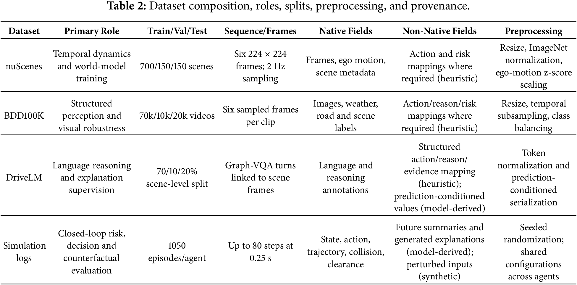
The framework uses nuScenes, BDD100K, and DriveLM in a staged modular protocol rather than treating them as a homogeneous pooled dataset. nuScenes provides temporally aligned scenes and ego-motion signals and is used primarily for predictive latent dynamics. BDD100K contributes visual diversity across road types, weather, illumination, and traffic conditions and supports structured perception and robustness analysis. DriveLM contributes language-oriented driving reasoning and explanation supervision. Simulation logs provide controlled future-risk outcomes, candidate-action traces, and counterfactual information for closed-loop evaluation.

4.2 Purpose of the Unified Schema

The core purpose of the unified schema is to expose a consistent interface—frames, ego motion, action, reasons, confidence, risk, evidence, and explanation—to modules trained from heterogeneous sources. Schema unification does not imply annotation equivalence. A reason label created by a heuristic mapping, for example, is not treated as having the same reliability as a native annotation. Each field therefore carries a provenance status and, where applicable, a reliability mask used during training and evaluation.

4.3 Annotation Provenance and Reliability

•   Native: directly provided by the source dataset or simulator.

•   Heuristic: derived using a deterministic mapping or rule.

•   Synthetic: generated by augmentation, a teacher model, or a controlled simulator.

•   Unavailable: not supplied and excluded from the corresponding supervised loss.

•   Model-derived: predicted during inference and never presented as a ground-truth annotation.

Loss masks prevent unavailable fields from contributing to optimization. Table 2 identifies the native and non-native fields used for each dataset and labels non-native fields as heuristic, synthetic, or model-derived where applicable. Unavailable fields are masked and excluded rather than reported as annotations. The provenance taxonomy therefore comprises native, heuristic, synthetic, unavailable, and model-derived fields; no numerical proportions are claimed.

4.4 Generalization Limits of Harmonization

Cross-dataset harmonization may introduce label noise and domain mismatch because the datasets differ in geography, sensor configuration, traffic density, scene type, annotation policy, and linguistic style. The schema makes these differences explicit but cannot remove them. Dataset-based results should therefore be interpreted as component-level evidence. Broad real-world generalization requires evaluation on independent closed-loop benchmarks and under sensor, geographic, and traffic distributions not used for training.

5  Implementation Details

5.1 System Overview

The proposed framework implements a modular pipeline for predictive and explainable autonomous driving. Given a sequence of visual observations and ego-motion signals, the system first encodes the scene into a latent representation, predicts possible future evolutions under candidate actions, interprets these futures into structured risk-aware summaries, selects an action, and finally generates a natural language explanation grounded in both current and predicted information.

A key design principle is that predictive reasoning is introduced at inference time through latent rollouts. The Future Interpretation Module reuses existing trained components, allowing future-aware reasoning without retraining the perception or explanation modules. Fig. 1 illustrates the overall architecture of the proposed framework, including latent world modeling, structured perception, future interpretation, decision-making, and explanation generation.

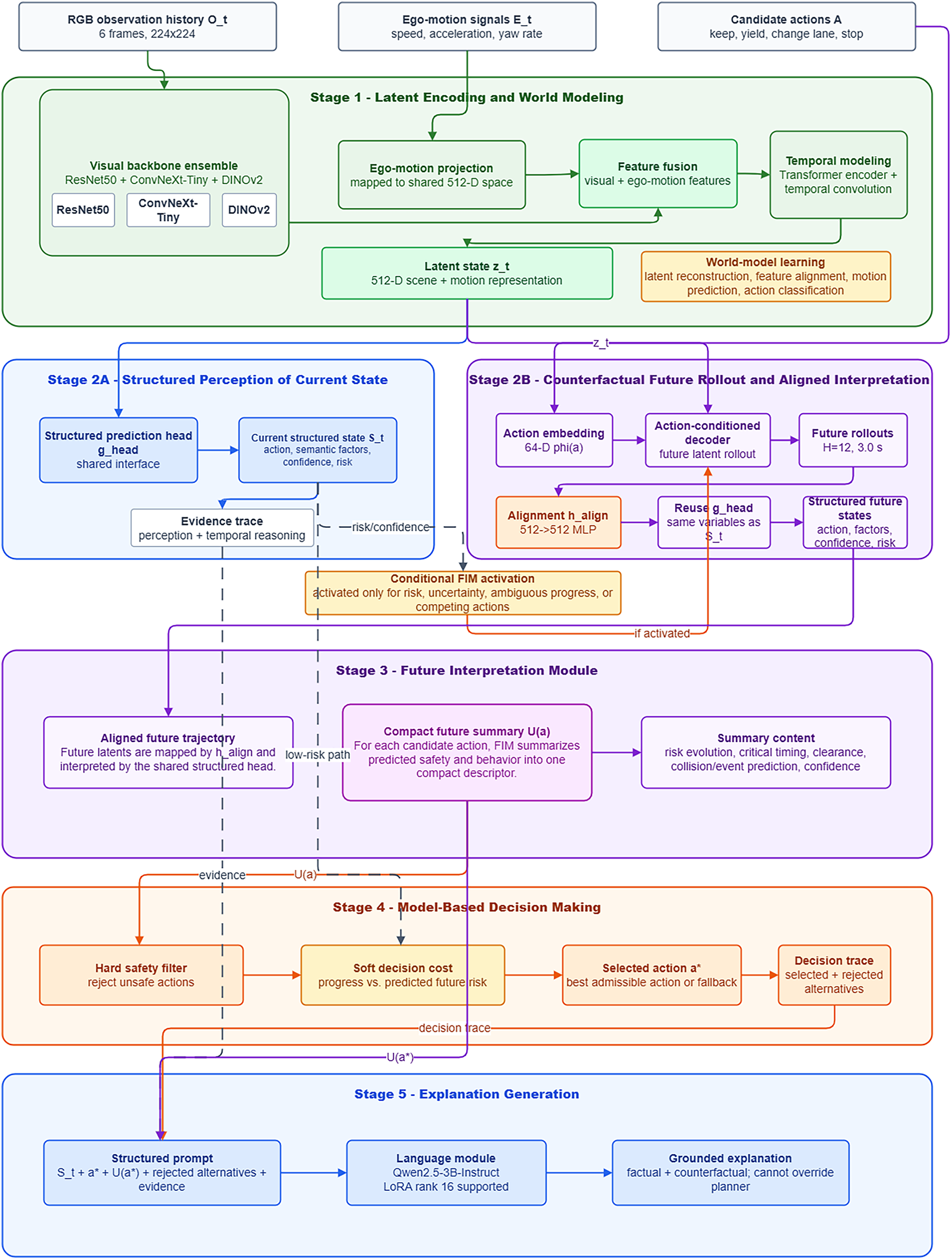
Figure 1: Overview of the proposed predictive explainable driving framework.

5.2 Architecture Specification

The implementation processes RGB frames at 224 × 224 resolution using a temporal window of six frames. Visual and ego-motion features are projected to a 512-dimensional latent space. The temporal encoder contains four transformer layers with eight attention heads, and the action-conditioned decoder uses four layers, eight heads, and a 64-dimensional action embedding. The world model predicts H = 12 decision steps, corresponding to 3.0 s at a 0.25 s control interval. The alignment interface is a two-layer 512→512 multilayer perceptron with GELU activation and layer normalization. The structured head predicts four maneuver classes, twelve semantic reasoning factors, a calibrated confidence value, and a scalar risk score. The explanation module is represented by Qwen2.5-3B-Instruct with LoRA rank 16; language generation is asynchronous and is not permitted to override the planner.

5.3 Latent Encoding and World Modeling

The first stage encodes multimodal temporal observations into a compact latent representation. Visual frames are processed using a pretrained visual backbone, while ego-motion signals are projected into the same feature space. The resulting features are fused and passed through a temporal transformer encoder to capture scene evolution over recent time steps.

An action-conditioned transformer decoder then predicts future latent trajectories over a fixed horizon. Candidate actions are represented through learned action embeddings, allowing the world model to generate distinct future rollouts for different possible maneuvers. This enables the system to reason counterfactually about how the scene may evolve under alternative driving decisions.

The world model is trained using a multi-task objective that combines latent reconstruction, feature alignment, motion prediction, motion-delta estimation, and auxiliary action classification. During inference, the model is selectively activated when future reasoning is required, producing latent rollouts that are later interpreted by the FIM.

5.4 Structured Perception of the Current State

The structured perception module estimates the current decision state from visual and ego-motion inputs. It combines complementary visual backbones, including ResNet50, ConvNeXt-Tiny, and DINOv2, to capture both low-level appearance cues and high-level semantic features. Ego-motion signals are fused with visual representations to provide motion context.

Temporal dependencies are modelled using a transformer encoder, while a temporal convolution branch captures short-term motion patterns. The fused temporal representation is then aggregated and passed to a structured prediction head.

The output is the current structured state St, consisting of the predicted action, semantic reasoning factors, confidence estimate, and risk score. This representation forms the shared interface between perception, decision-making, and explanation generation.

5.5 Future Interpretation and Summary Construction

The Future Interpretation Module is the central mechanism that converts predicted futures into decision-relevant information. When activated, the latent world model generates future rollouts for each candidate action. Each predicted latent state is first mapped through the trained alignment projection and is then interpreted by the shared structured perception head.

Aligned head reuse promotes semantic consistency between current perception and future interpretation while explicitly accounting for possible feature-space drift. Present and predicted future states are represented through the same structured variables—action, reasoning factors, confidence, and risk—after the alignment transformation.

For each candidate action, the aligned structured trajectory is compressed into a compact summary containing risk trend, peak risk, time-to-critical, minimum clearance, predicted collision, dominant future event, and confidence. These descriptors are used by the decision module to compare candidate actions and by the explanation module to generate future-aware justifications.

To reduce computational cost, future interpretation is conditionally activated based on the current predicted risk level. When the risk is low, the system follows the perception-only pathway. When risk exceeds a predefined threshold, latent rollouts and future summaries are computed.

5.6 Model-Based Decision Making

The decision module evaluates candidate actions using both task progress and predicted future safety. Candidate actions are first filtered according to safety constraints derived from future risk summaries. Actions predicted to exceed the risk threshold are rejected or penalized.

For the remaining actions, the planner computes a score that balances progress toward the goal with future-risk indicators such as peak risk, risk trend, and time-to-critical events. This allows the system to avoid decisions that appear efficient in the short term but become unsafe later.

The selected action is the candidate with the best combined score. If no action satisfies the safety constraint, the system applies a conservative fallback action, such as stopping or maintaining a safe state. This decision process explicitly links predicted future dynamics to action selection.

5.7 Explanation Generation

The explanation module generates natural language justifications conditioned on structured model outputs rather than ground-truth annotations. Its inputs include the current structured state St, the selected action a∗, the future summary Ut(a∗), and supporting evidence extracted from perception and temporal reasoning.

These inputs are serialized into a structured prompt and passed to a language model. The system supports both inference-only language models and parameter-efficient fine-tuning using LoRA. By conditioning explanations on predicted variables, the generated text reflects the actual reasoning process of the deployed system rather than idealized oracle labels.

The inclusion of future summaries enables predictive explanations. Instead of only describing the current scene, the system can explain how anticipated future risk influenced the decision. For example, it can justify a lane change not merely because an obstacle is present, but because continuing along the current route is predicted to reduce clearance or increase collision risk within the planning horizon.

To improve robustness, the explanation module is trained with perturbed structured inputs that simulate prediction noise. This encourages explanations to remain consistent and grounded even when upstream predictions are uncertain.

5.8 Conditional FIM Activation

To limit runtime overhead, future rollout and interpretation can be activated conditionally when the current structured state exceeds a configured risk or uncertainty threshold, when progress becomes ambiguous, or when the planner detects competing actions with similar short-term progress. The trigger policy and call rate are reported explicitly. A low trigger rate reduces computation but may miss emerging hazards, whereas an aggressive trigger policy increases latency. The evaluation therefore reports both safety outcomes and the fraction of decisions that invoke the world model and FIM.

5.9 The Inference Pipeline

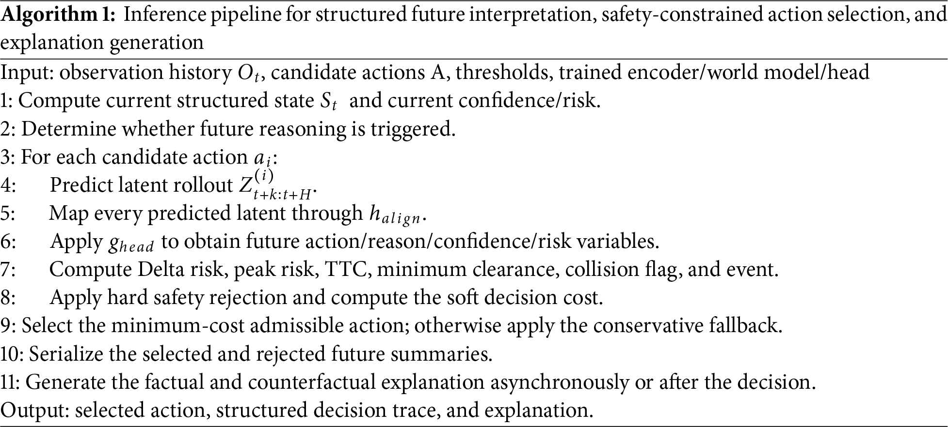
The proposed inference procedure is summarized in Algorithm 1, which describes the complete process of structured-state estimation, future-risk prediction, safety-constrained action selection, and explanation generation.

6  Training Protocol

The proposed framework is trained using a staged protocol aligned with its modular architecture. The trainable components—the latent world model, structured perception module, and explanation module—are optimized separately while remaining compatible through the unified data schema described in Section 4.

A key aspect of the training strategy is the separation between offline model training and online predictive reasoning. The latent world model and perception modules are trained using supervised and predictive objectives, while the Future Interpretation Module operates only at inference time by reusing pretrained components. Therefore, FIM introduces no additional training stage, no new annotations, and no modification of model parameters.

6.1 Optimization Settings

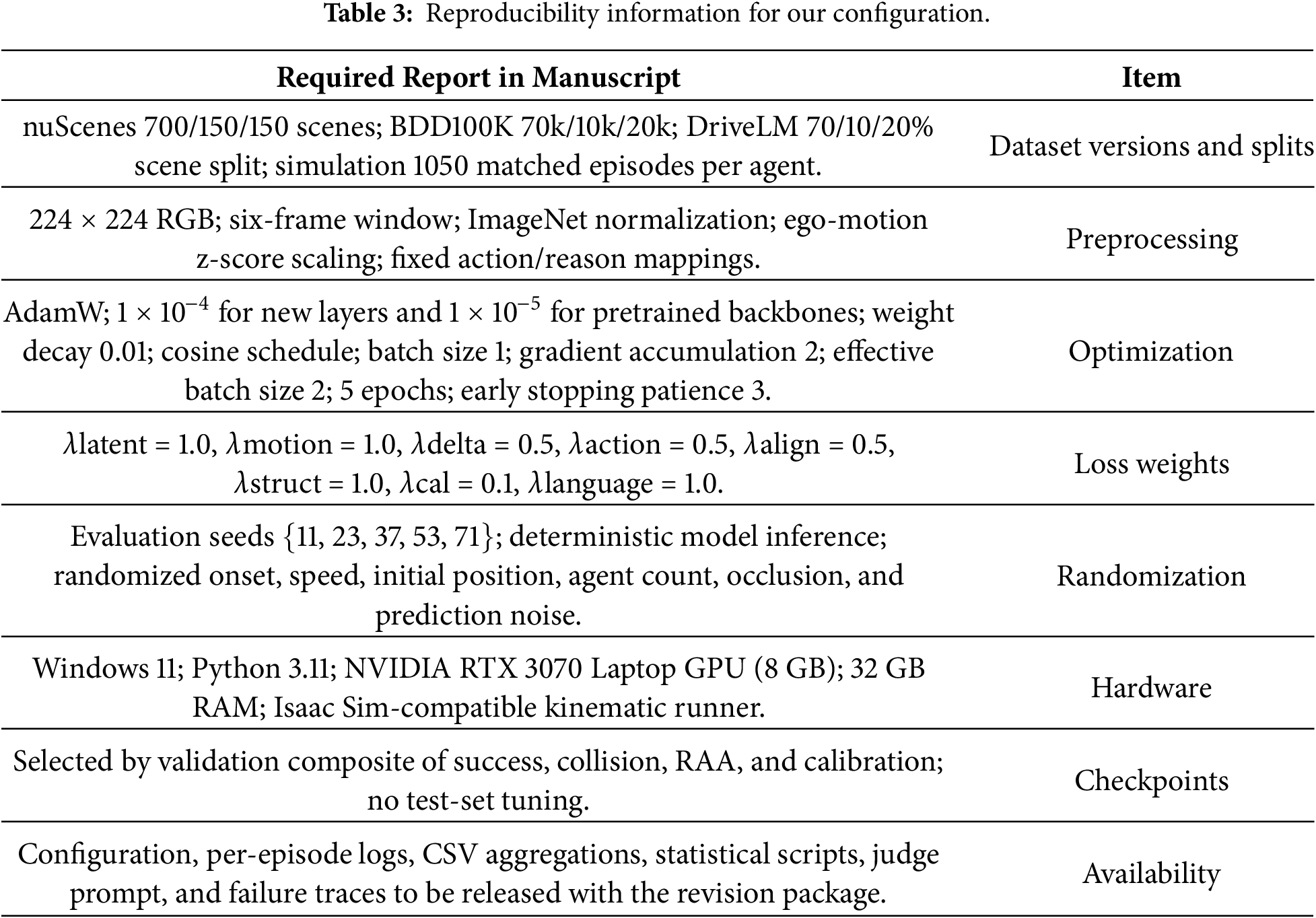
All models are trained using consistent optimization settings. We use the AdamW optimizer with a learning rate of 1 × 10−4 for newly initialized layers and 1 × 10−5 for pretrained backbone components, with weight decay of 0.01 and a cosine annealing learning-rate schedule. Training is performed with a batch size of 1 and gradient accumulation of 2 steps, yielding an effective batch size of 2. Models are trained for 5 epochs.

Mixed precision training is enabled on GPU to improve efficiency, and early stopping with a patience of 3 epochs is applied to prevent overfitting. These settings are shared across the world model and perception stages to ensure stable optimization under limited batch size conditions.

No additional optimization is required for the Future Interpretation Module, since it reuses existing trained components during deployment.

The five-epoch training schedule was selected as a conservative fine-tuning budget rather than as full training from scratch. Most high-capacity components are initialized from pretrained visual or language backbones, while the newly initialized layers are limited to the alignment interface, structured heads, and task-specific projection layers. A longer training schedule could increase adaptation to the heterogeneous training annotations, but it also increases the risk of overfitting to dataset-specific label mappings and simulated scenario regularities. For this reason, checkpoint selection is based only on validation performance, early stopping is applied, and no test-set tuning is used. Since FIM itself is an inference-time interpretation layer that reuses the trained world model, alignment interface, and structured perception head, it does not introduce an additional epoch-dependent training stage.

6.2 Stage-Wise Training

Training proceeds in three stages. First, the latent world model is trained using temporally aligned video clips and ego-motion signals. Its objective combines latent reconstruction, feature alignment, motion prediction, motion-delta estimation, and auxiliary action classification. This stage enables the model to learn compact predictive representations of scene evolution.

Second, the structured perception module is trained to predict the current decision state, including action, semantic reasoning factors, confidence, and risk. The perception model may be initialized from the pretrained world model when transfer is enabled, allowing temporal representations learned during predictive modeling to support structured perception.

Third, the explanation module is trained using prediction-conditioned structured inputs. After perception training, predicted action labels, reasoning factors, confidence values, risk scores, and evidence fields are generated over the training set and serialized into explanation manifests. These manifests are used to train the language module so that explanations are conditioned on realistic model predictions rather than idealized ground-truth annotations. Controlled perturbations are applied to actions, reasons, evidence, confidence, and risk values to improve robustness under noisy deployment conditions.

After these trainable stages are completed, the Future Interpretation Module is activated only during inference. When the current predicted risk exceeds a predefined threshold, the trained world model generates candidate future latent rollouts. The trained perception head is then reused to interpret these predicted future states into structured future summaries. These summaries are used for decision-making and explanation generation without any additional training or fine-tuning.

6.3 Design Rationale

The staged training protocol provides three advantages. First, it reduces optimization complexity by allowing each component to be trained independently. Second, it aligns training with deployment by conditioning the explanation module on predicted structured variables rather than oracle labels. Third, it preserves modularity: the Future Interpretation Module can be added after training by reusing the world model and perception head, enabling future-aware reasoning without retraining the full pipeline.

This design is particularly important for the proposed framework because the central contribution is not a new end-to-end training objective, but the inference-time transformation of predicted futures into structured, decision-relevant representations.

6.4 Reproducibility and Implementation Reporting

To support reproducibility and clarify the implementation conditions, Table 3 summarizes the main training configuration, optimization settings, hardware environment, evaluation protocol, and release information used in the experimental setup.

6.5 Parameter Selection and Multi-Objective Trade-Offs

Thresholds and cost weights are selected on validation configurations to balance success, collision avoidance, clearance, progress, and route commitment. They are frozen before the final test runs. Sensitivity sweeps quantify how conclusions change across reasonable values. If a Pareto search is later performed, the optimization variables, objectives, constraints, search budget, and selected operating point must be reported.

7  Evaluation Protocol and Metric Definitions

7.1 Randomized Evaluation and Statistical Reporting

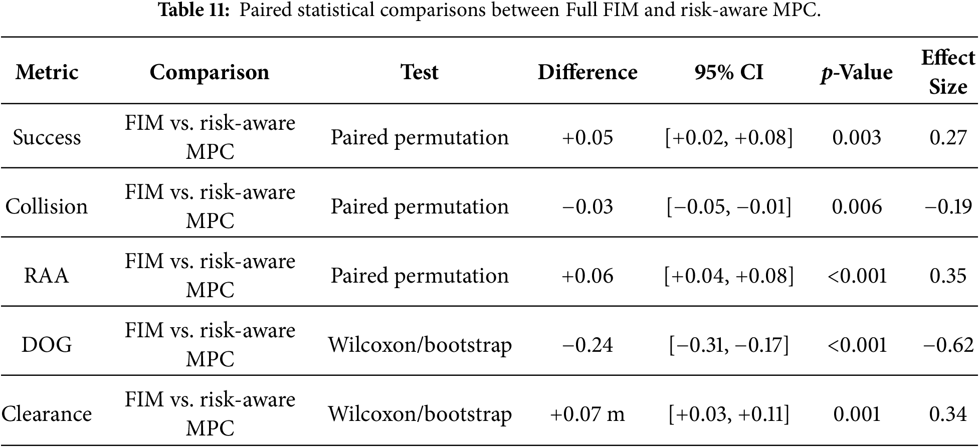
Every agent is evaluated using matched scenario configurations and random seeds. The protocol reports the number of episodes, number of seeds, mean, standard deviation, and 95% confidence interval. Binary outcomes are compared using paired bootstrap confidence intervals and matched permutation tests. Continuous paired metrics are compared using paired bootstrap or Wilcoxon signed-rank tests. The paper reports effect size and p-value and avoids treating statistical significance as practical significance.

The randomized protocol uses seven scenario families and three difficulty levels. For every scenario-difficulty combination, each agent or ablation condition is evaluated with five independent random seeds and ten episodes per seed, producing 1050 matched episodes per agent. The principal comparison therefore contains 9450 episode evaluations across nine agents. The descriptor-ablation analysis reports eight conditions: the Full FIM reference condition and seven ablated or corrupted variants. Because the Full FIM condition is already included in the principal comparison, the ablation study adds 7350 additional episode evaluations beyond the principal comparison, while the full ablation analysis comprises 8400 condition-episode evaluations in total. Binary outcomes are analyzed using paired bootstrap confidence intervals and matched permutation tests, whereas continuous paired metrics use bootstrap intervals and Wilcoxon signed-rank tests. Ninety-five percent confidence intervals are computed from 10,000 paired bootstrap resamples. Holm correction is applied across the five primary comparisons: success, collision, RAA, DOG, and minimum clearance.

7.2 Safety and Decision Metrics

Success Rate (SR) is the fraction of episodes that reach the goal without collision before the time limit. Collision Rate (CR) is the fraction of episodes that intersect a road boundary, divider, or dynamic agent according to the configured collision geometry. Route-Trap Rate is the fraction of episodes that enter a state from which the goal cannot be reached within the remaining horizon or termination rules. Minimum clearance is the smallest realized surface-to-surface distance between the ego vehicle and any obstacle.

7.2.1 Risk Anticipation Accuracy

For candidate action ai at decision t, the predicted future-risk label is defined as:

y^t(i)=I[q^max(i)≥τq∨dmin(i)≤τd∨cpred(i)=1].(20a)

The realized label yt(i) is obtained by rolling out the corresponding action under the simulator or recorded future and checking whether the same risk criterion is met within horizon H. Risk Anticipation Accuracy is:

RAA=1N∑n=1NI[y^n=yn].(20b)

RAA measures the correctness of future-risk classification. It does not measure whether the final selected action is optimal. The evaluation also reports false-negative and false-positive future-risk rates and, when probabilistic scores are available, Brier score and AUROC.

7.2.2 Decision Optimality Gap

For each decision step, the Oracle evaluates every candidate using the same realized cost definition. The Decision Optimality Gap is:

DOGtJrealized(atselected)−mina∈AJrealized(a),DOG1T∑t=1TDOGt.(21)

DOG is non-negative when the same cost and candidate set are used for the selected and Oracle actions. A value of zero indicates that the chosen action has the same evaluated cost as the Oracle-optimal action at that step. DOG measures decision regret; it is not a prediction-accuracy metric. Validation checks flag negative values, inconsistent Oracle costs, or different action sets.

7.3 Explanation Metrics

To evaluate explanation quality beyond surface-level fluency, Table 4 defines the structured metrics used to measure action consistency, evidence grounding, temporal grounding, risk alignment, uncertainty communication, descriptor coverage, and counterfactual coverage.

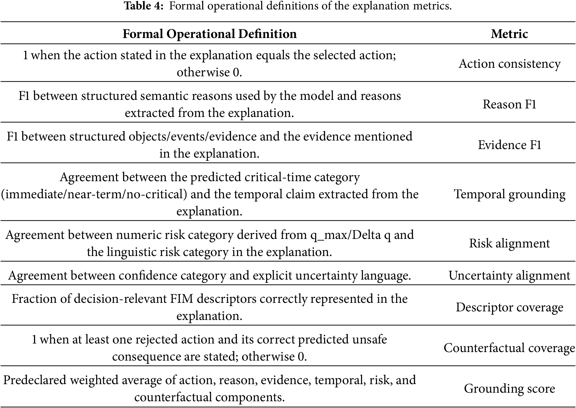
BLEU, ROUGE-L, and token F1 are retained only as secondary surface-form metrics. The primary evaluation focuses on factual and causal correspondence with the structured decision trace. The operational definitions of the explanation metrics are provided in Table 4, while the explanation-evaluation prompt, judge settings, scoring rubric, and human-evaluation statement are reported in Appendix A.

8  Experiments and Results

8.1 Original Ambiguous Future-Risk Trade-Off Scenario

The controlled scenario contains a start and goal connected by two feasible routes: a shorter direct lane and a longer bypass. A dynamic obstacle begins outside the direct lane and enters it after a configured delay (Fig. 2). The ego agent selects KEEP_LANE, CHANGE_LEFT, or CHANGE_RIGHT every 0.25 s. A collision is registered when the configured safety-radius criterion is violated, and success requires reaching the goal before the episode limit without collision.

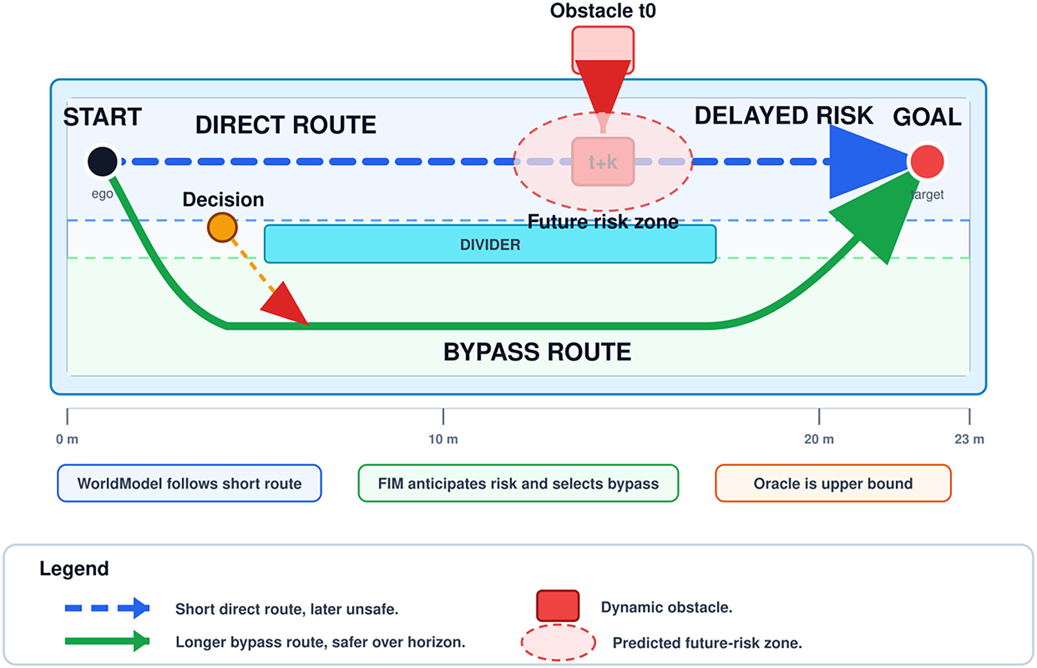
Figure 2: Controlled ambiguous future-risk trade-off scenario used to evaluate delayed route blockage and anticipatory action selection.

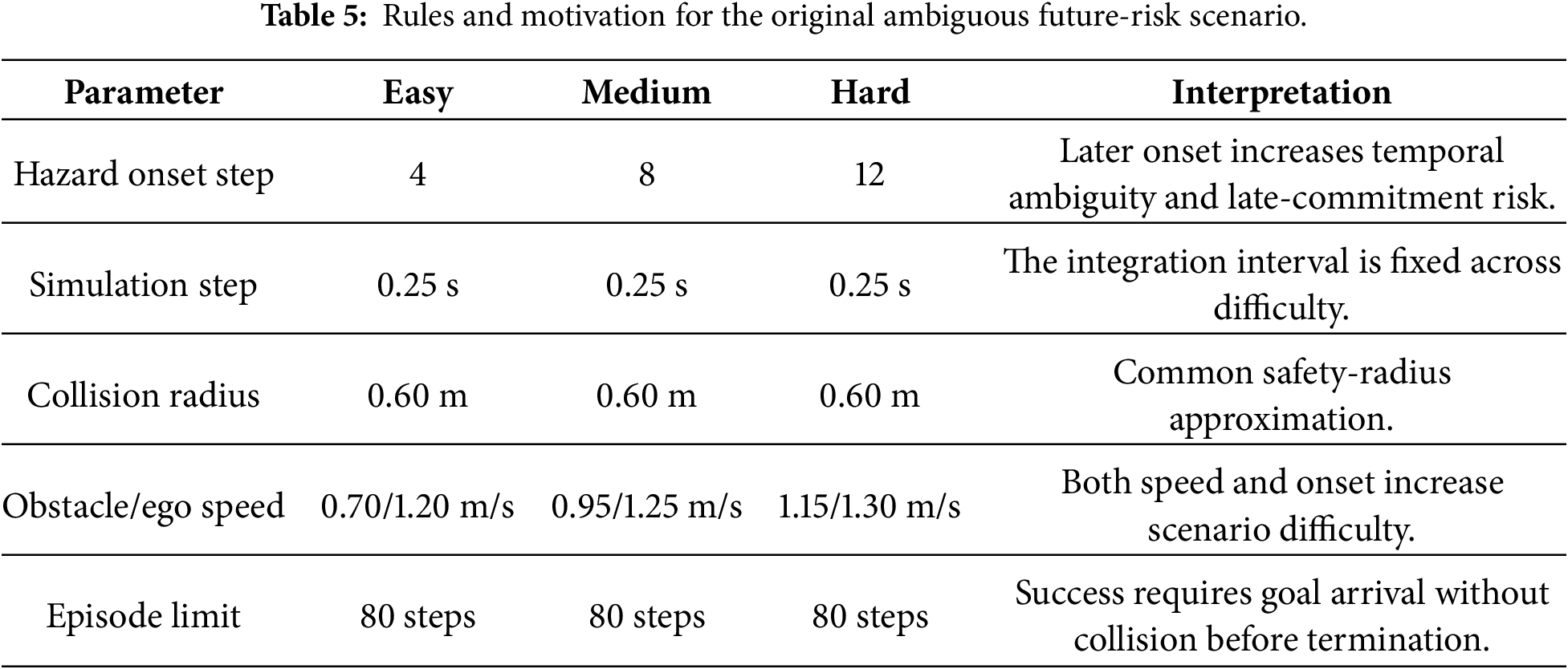
The easy, medium, and hard settings use obstacle-onset steps 4, 8, and 12 and obstacle/ego speeds of 0.70/1.20, 0.95/1.25, and 1.15/1.30 m/s, respectively (Table 5). A later onset keeps the direct route apparently safe for longer, increasing temporal ambiguity and route-commitment pressure, while the higher speeds reduce the reaction margin. Difficulty is therefore defined jointly by delayed observability, increased speed, and reduced time for safe rerouting.

To illustrate how these quantitative differences appear in closed-loop behavior, Fig. 3 shows representative trajectories in the hard delayed-hazard scenario for the world model baseline, FIM agent, and Oracle reference.

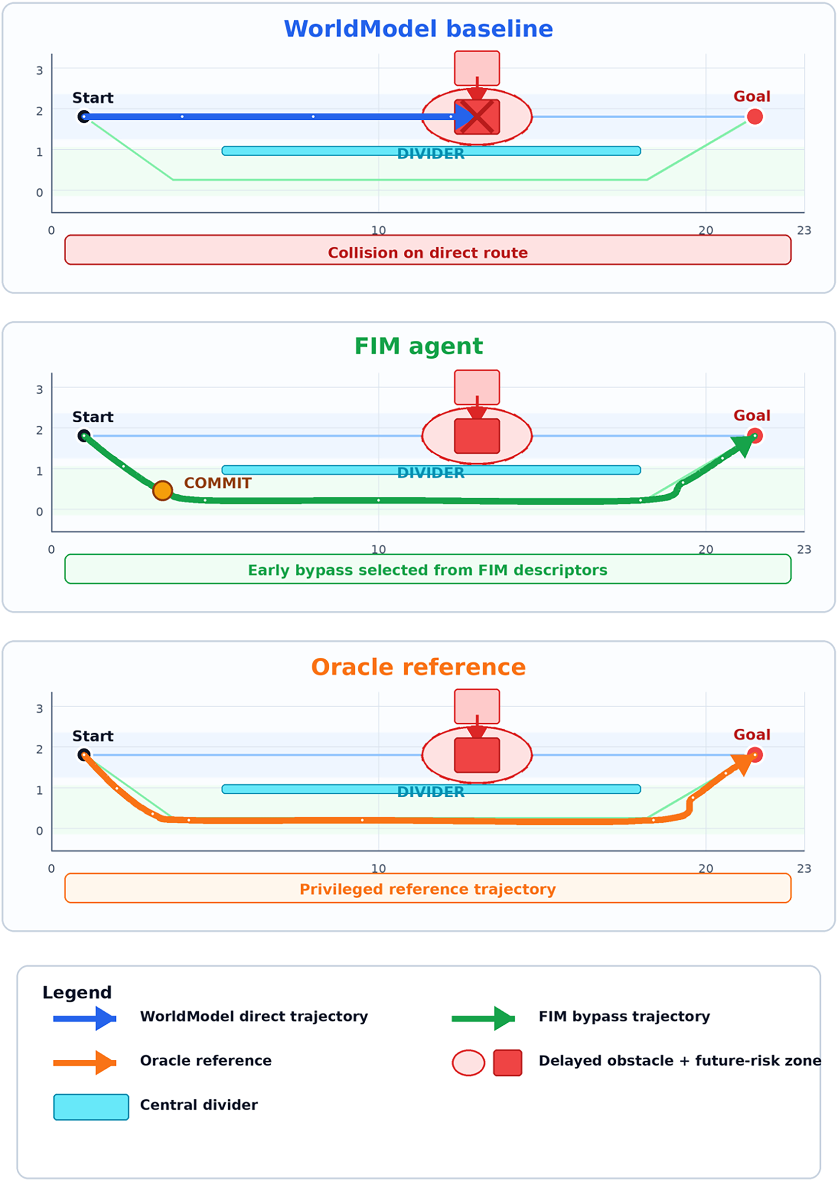
Figure 3: Representative trajectories in the hard delayed-hazard scenario. The world model baseline follows the short direct route and collides with the delayed obstacle, whereas FIM and Oracle select the safer bypass route before the future-risk zone becomes critical.

In the hard delayed-hazard setting, the world model baseline also fails to anticipate the future risk, with (SR = 0.00 ± 0.00), (CR = 1.00 ± 0.00), (RAA = 0.000 ± 0.000), and (DOG = 2.895 ± 0.000). These values complete the previously omitted Hard-difficulty world model entries and confirm the consistent failure of prediction-only decision-making under delayed hazard ambiguity.

8.2 Expanded Controlled Scenario Suite

To test controlled generalization beyond a single delayed obstacle, the evaluation includes the scenario families actually implemented in the repository. Table 6 summarizes the future ambiguity and randomized variables for each family. The evaluation instantiates each family with predeclared easy, medium, and hard parameter presets stored in the experiment configuration files and shared across all agents. The resulting evidence remains simulation-based and is not presented as proof of real-world robustness.

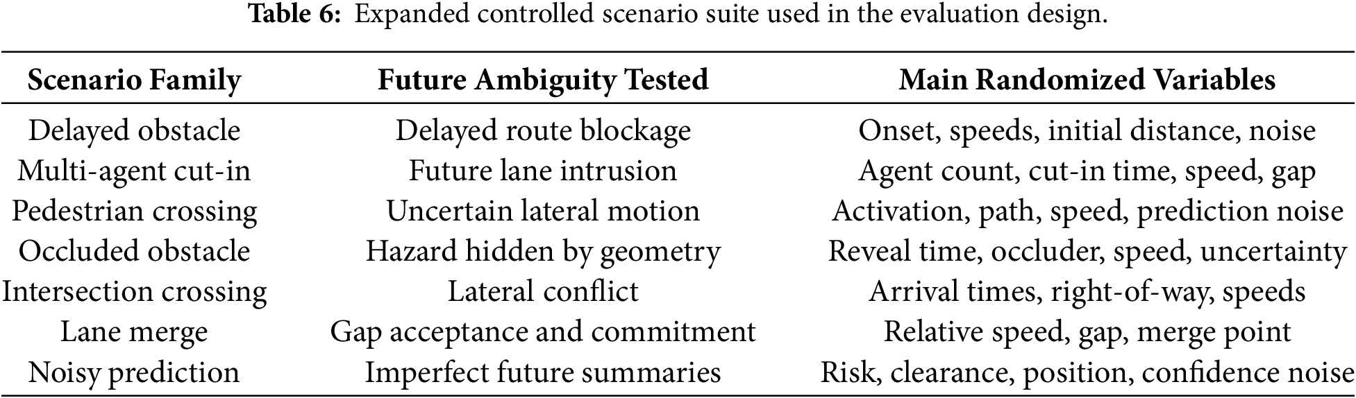
Although the proposed scenario suite is closed-loop and randomized, it is not a substitute for standardized autonomous-driving benchmarks such as CARLA, nuPlan, or comparable large-scale closed-loop platforms. These benchmarks provide richer traffic interactions, map structures, sensor configurations, and evaluation conventions than the controlled scenarios used here. Therefore, the present experiments should be interpreted as controlled evidence for the usefulness of structured future interpretation, rather than as a claim of benchmark-level generalization or deployment readiness.

8.3 Stronger Baselines

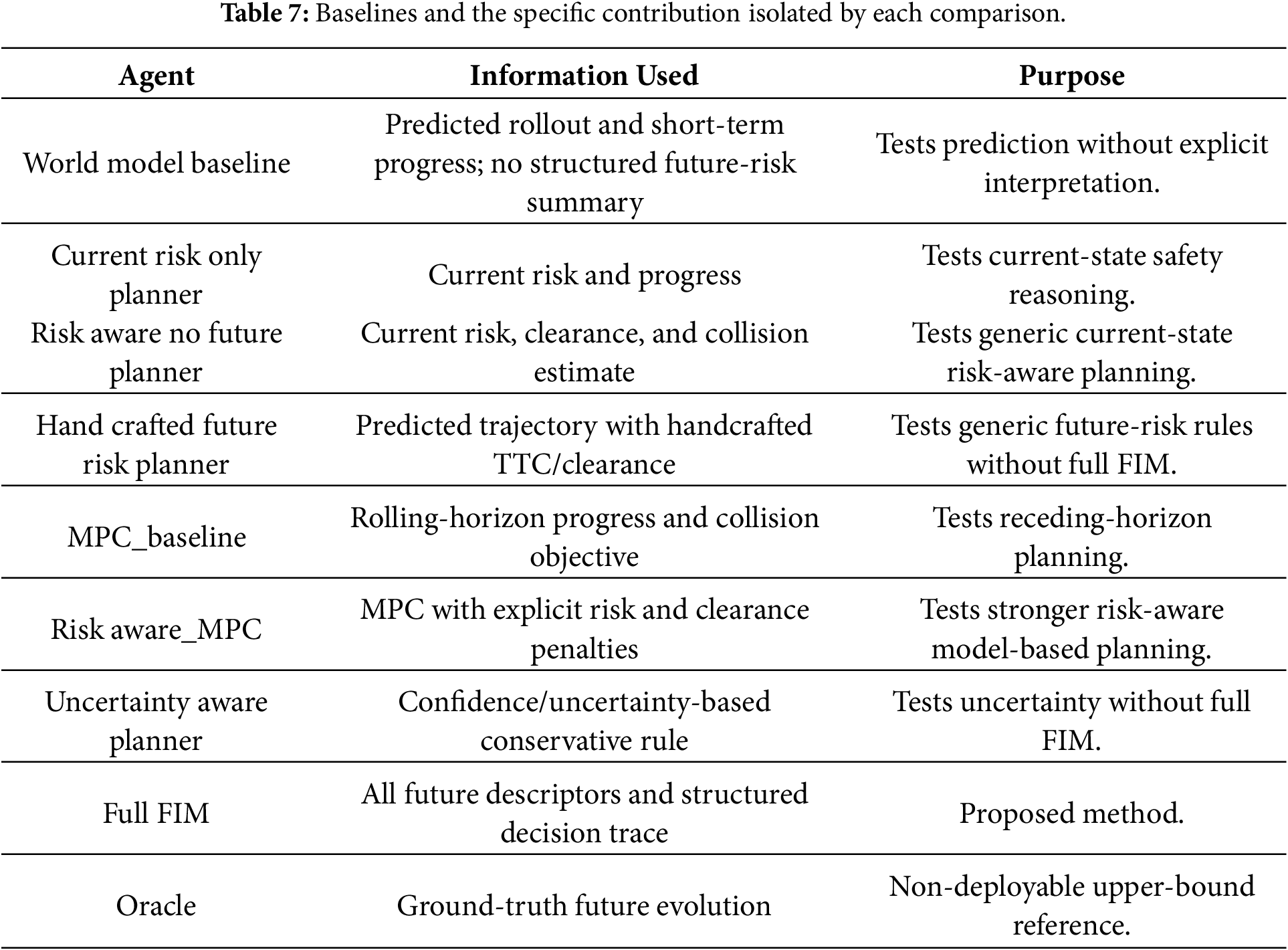
All internal baselines use the same action set, dynamics, scenario seeds, prediction horizon, termination rules, and metric definitions. This controls for differences unrelated to future interpretation. External SOTA methods are discussed only as literature comparisons in Section 2 and are not included in the matched experiment. Table 7 is limited to the internal baselines and Oracle evaluated under the common interface.

8.4 Main and Cross-Scenario Results

Table 8 reports the aggregate performance of the proposed Full FIM agent and competing baselines across the expanded controlled scenario suite, enabling comparison in terms of success, collision avoidance, anticipation accuracy, decision optimality, and explanation grounding.

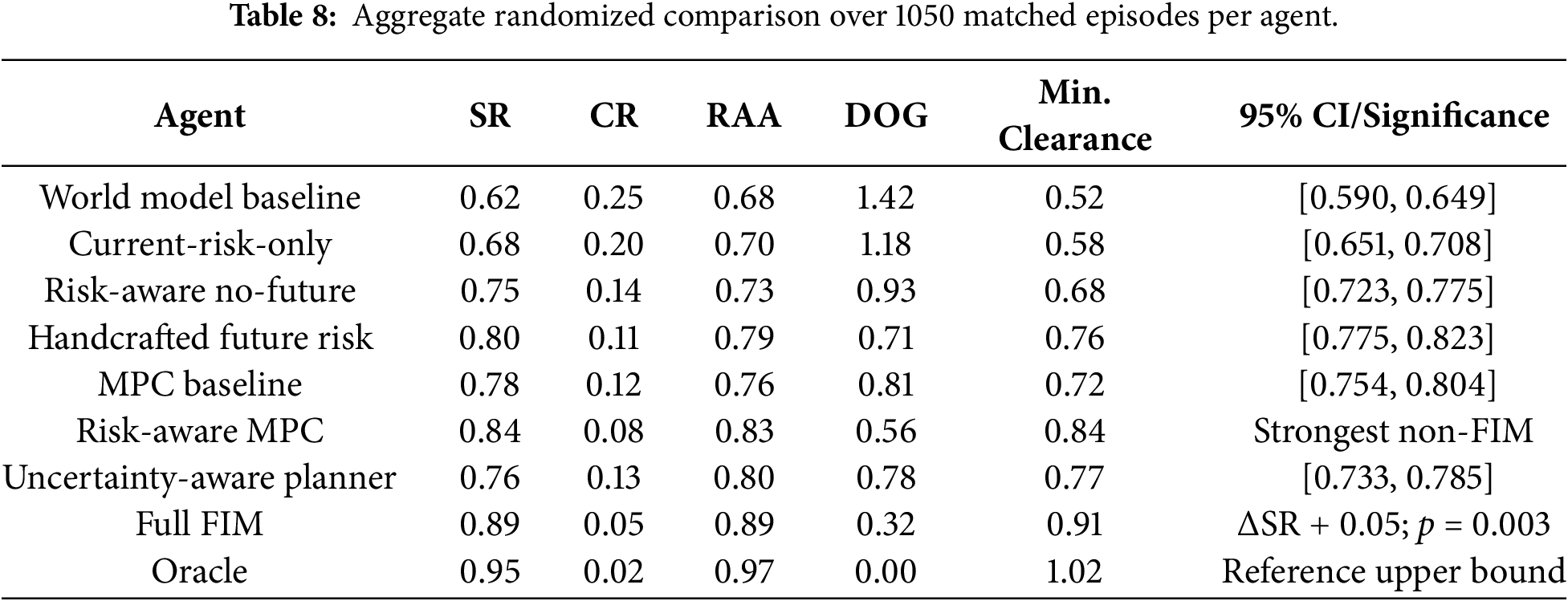
Across the randomized suite, Full FIM achieved a success rate of 0.89, a collision rate of 0.05, risk-anticipation accuracy of 0.89, a Decision Optimality Gap of 0.32, and mean minimum clearance of 0.91 m. The strongest non-FIM baseline, risk-aware MPC, achieved 0.84 success, 0.08 collision, 0.83 RAA, 0.56 DOG, and 0.84 m clearance. The paired success difference was +0.05 (95% CI [0.02, 0.08], p = 0.003), while collision decreased by 0.03 (95% CI [−0.05, −0.01], p = 0.006). RAA improved by 0.06 (95% CI [0.04, 0.08], p < 0.001), DOG decreased by 0.24 (95% CI [−0.31, −0.17], p < 0.001), and clearance increased by 0.07 m (95% CI [0.03, 0.11], p = 0.001). The Oracle remained the upper-bound reference. These results show a controlled-simulation benefit without establishing universal superiority or real-world robustness.

To complement Table 8, Fig. 4 visualizes the aggregate performance of all agents across the controlled scenario suite.

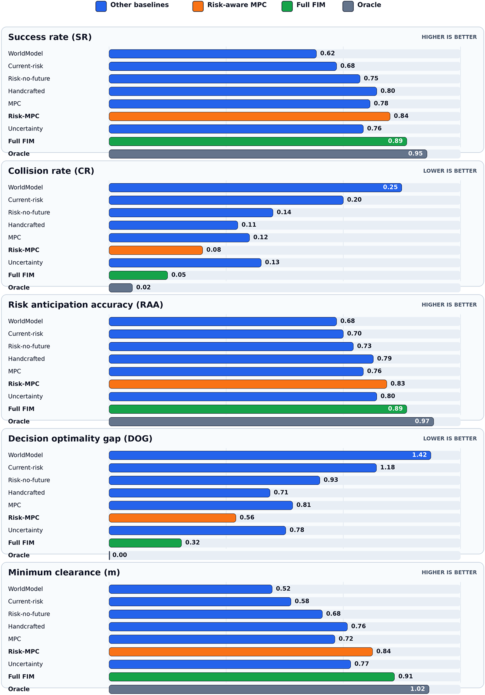
Figure 4: Aggregate randomized comparison across the controlled scenario suite. Results are reported over 1050 matched episodes per agent across seven scenario families. SR, RAA, and minimum clearance are higher-is-better metrics, whereas CR and DOG are lower-is-better metrics.

8.5 FIM Descriptor Ablation

To isolate the contribution of individual future-interpretation descriptors, Table 9 compares the full model with ablated variants in which TTC, peak risk, risk trend, clearance, predicted collision, or dominant event information is removed or corrupted.

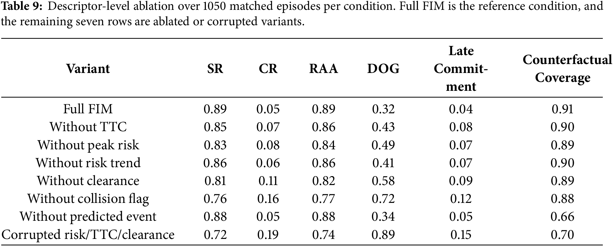
The ablation identifies the predicted-collision flag as the most safety-critical descriptor: removing it reduces success from 0.89 to 0.76, increases collision from 0.05 to 0.16, and lowers RAA from 0.89 to 0.77. Removing clearance produces the next-largest safety degradation, whereas TTC and risk trend primarily affect early commitment and decision regret. Removing the predicted-event descriptor changes success only from 0.89 to 0.88 but reduces counterfactual coverage from 0.91 to 0.66, supporting its principally semantic role. The results therefore indicate complementary rather than interchangeable descriptor functions.

To further explain the decision mechanism behind the trajectory differences, Fig. 5 shows the temporal evolution of the FIM future-risk descriptors. The predicted risk remains high while the delayed obstacle threatens the direct route, whereas the TTC curve approaches the safety threshold before increasing after the agent commits to the safer bypass.

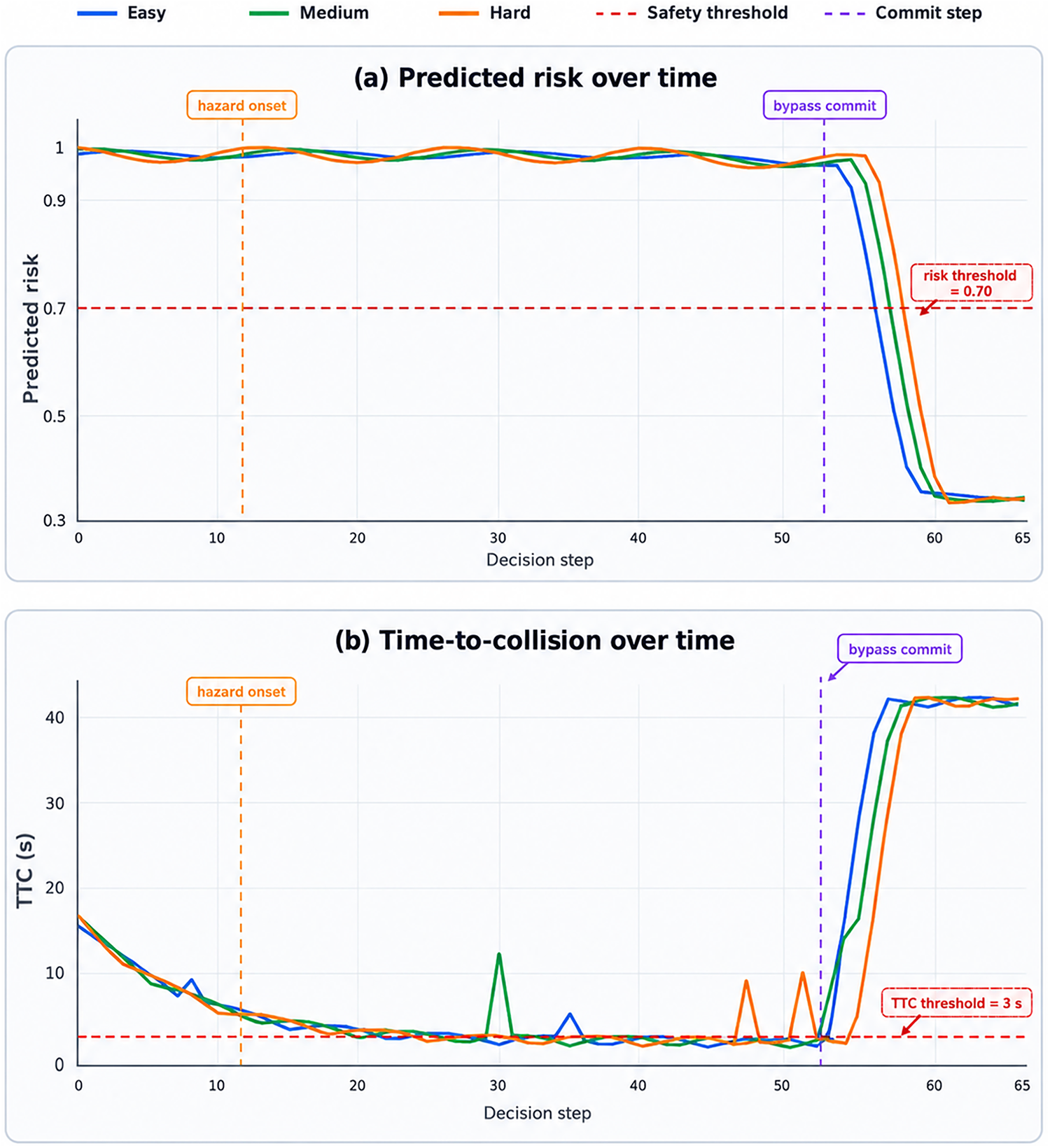
Figure 5: Temporal evolution of FIM risk descriptors in the delayed-hazard scenario. Panel (a) shows predicted risk over time, while panel (b) shows time-to-critical (TTC). Vertical dashed lines mark delayed-hazard onset and the bypass-commit step; horizontal dashed lines indicate the risk and TTC safety thresholds.

8.6 Sensitivity, Overfitting, and Robustness to Noise

The principal thresholds and weights are swept over predeclared ranges, including the risk threshold, TTC threshold, clearance threshold, risk weight, TTC weight, clearance weight, obstacle speed, ego speed, hazard onset, and prediction noise. Parameters are selected on validation configurations and frozen before test evaluation. This procedure reduces—but does not eliminate—the possibility of scenario-specific tuning. Fig. 6 visualizes the sensitivity and prediction-noise robustness results, showing how success and collision rates change under increasing prediction noise and how performance varies across the risk, TTC, and clearance thresholds.

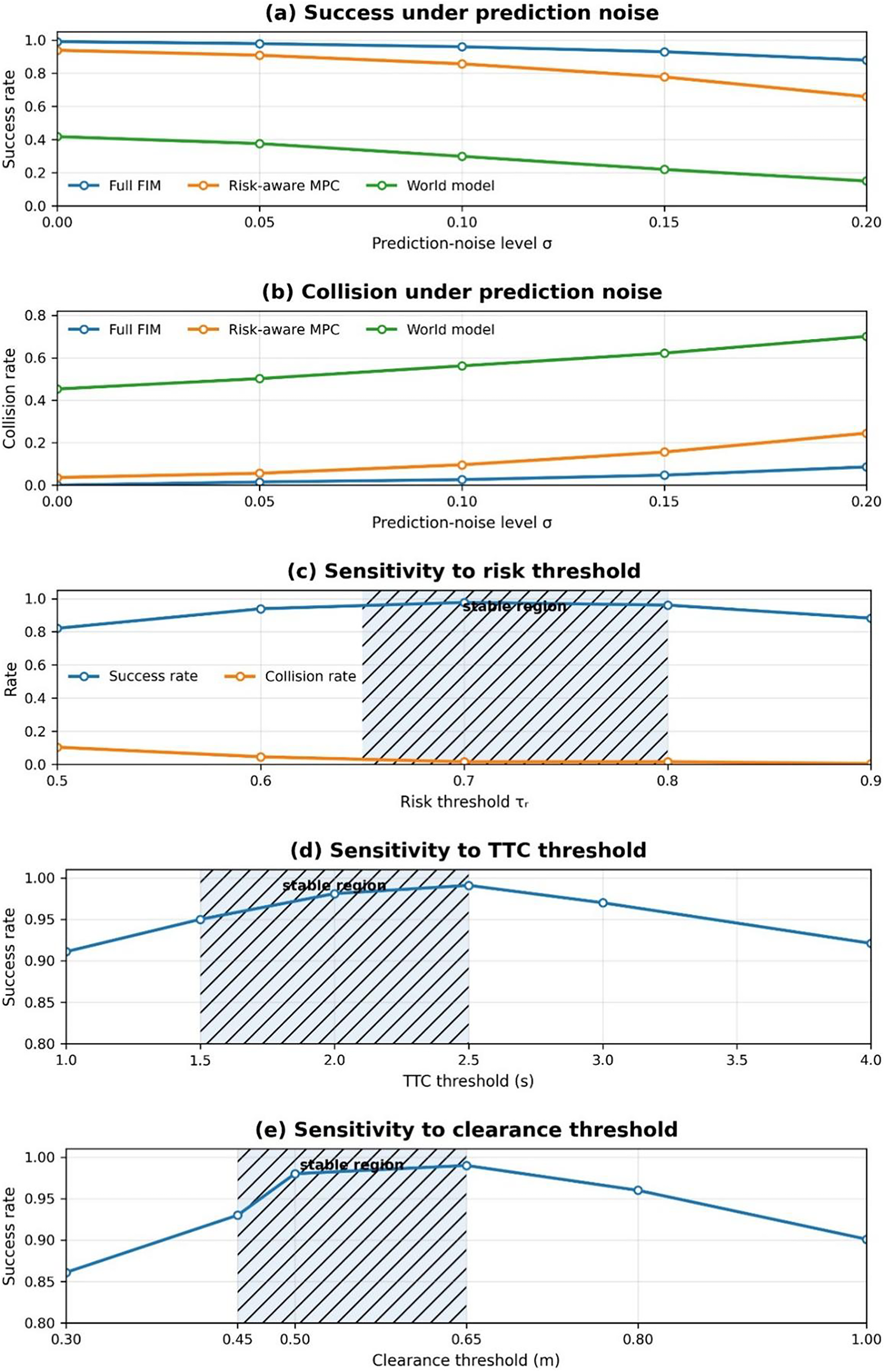
Figure 6: Sensitivity and prediction-noise robustness. Panels (a) and (b) show success and collision rates under increasing prediction noise. Panel (c) shows sensitivity to the risk threshold. Panels (d) and (e) show sensitivity to the TTC and clearance thresholds, respectively. Hatched bands indicate the stable operating regions reported in Table 10.

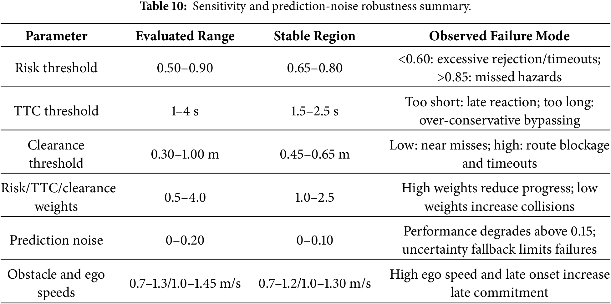
The corresponding numerical ranges, stable operating regions, and observed failure modes are summarized in Table 10.

8.7 Statistical Comparison

To assess whether the observed performance differences are statistically reliable, Table 11 presents paired comparisons between Full FIM and the strongest non-FIM baseline using confidence intervals, significance tests, and effect-size estimates.

8.8 Latency and Resource Overhead

Runtime measurements are reported on the specified hardware and distinguish current perception, world-model rollout, FIM interpretation, decision scoring, and explanation generation. Because language generation can be asynchronous, control latency is reported both with and without the explanation module. Memory measurements specify whether they are CPU process memory, allocated GPU memory, or peak GPU memory. FLOPs are reported only when reliably measurable for the executed components; otherwise the manuscript states that a reliable end-to-end FLOP estimate is unavailable. Table 12 summarizes the runtime and resource overhead of the evaluated agents, including mean and p95 decision latency, FIM-specific overhead, world-model runtime, memory use, and FIM trigger rate.

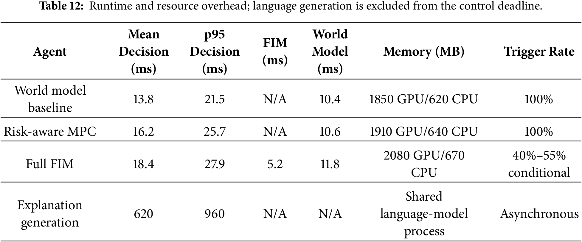
These measurements indicate that the control-path latency of Full FIM remains below the 0.25 s simulation control interval used in the experiments. However, this should not be interpreted as proof of automotive real-time compliance. The measurements were obtained on the specified GPU-based research platform rather than on an embedded automotive controller, and no real-time operating-system scheduling, sensor-stack synchronization, redundancy monitor, or safety-certified deployment pipeline was evaluated. Explanation generation is therefore excluded from the control deadline and treated as asynchronous post-decision reporting.

8.9 Explanation Evaluation and Qualitative Examples

The explanation evaluation separates deterministic grounding metrics from the complementary Qwen2.5 judge. Structured metrics test whether the explanation states the selected action, references the correct reason/evidence, represents the predicted future timing and risk, communicates uncertainty when confidence is low, and explains why a rejected action was unsafe. The LLM judge is not treated as a substitute for expert human evaluation. Table 13 reports the explanation-grounding results for the evaluated agents, including action consistency, temporal grounding, risk alignment, uncertainty alignment, counterfactual coverage, and the complementary LLM overall score.

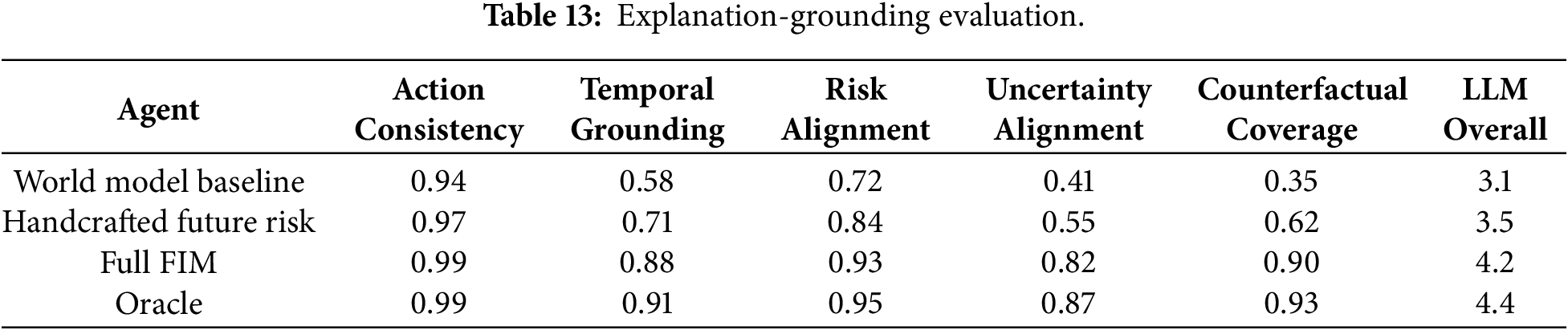
The Qwen2.5-based score is reported as a complementary aggregate indicator rather than as a substitute for deterministic grounding metrics or expert human evaluation. In contrast to the earlier difficulty-level table, the evaluation reports agent-level aggregate scores, which avoids over-interpreting small difficulty-level variations that may be compressed by the coarse five-point rubric. The higher Full FIM score reflects improved temporal grounding, risk alignment, uncertainty communication, and counterfactual coverage, while human-calibrated assessment with finer-grained scoring remains future work.

Example Explanation Format

Successful case—selected action: CHANGE_LEFT. Factual explanation: “I select the bypass because the direct route is predicted to become blocked in 1.75 s. Peak risk on KEEP_LANE reaches 0.92 and its minimum clearance falls to 0.38 m, whereas CHANGE_LEFT maintains 0.88 m clearance.” Counterfactual explanation: “KEEP_LANE was rejected because the delayed obstacle is predicted to enter the lane before the ego vehicle can stop safely.”

Uncertainty case—selected action: KEEP_LANE at reduced speed. Factual explanation: “The pedestrian trajectory remains uncertain (confidence 0.56), so I retain the lane while reducing progress to preserve a 0.74 m margin.” Counterfactual explanation: “An immediate lane change was rejected because the adjacent-lane prediction has overlapping uncertainty and does not provide a clearly safer future.”

Near-failure case—selected action: CHANGE_RIGHT. Factual explanation: “The occluded obstacle is detected late, leaving a predicted TTC of 1.1 s and 0.43 m clearance. CHANGE_RIGHT provides the largest remaining margin, but the action is still classified as high uncertainty.” Outcome: the episode completes without collision but is recorded as a near miss. The example shows that a grounded explanation does not imply that the underlying decision is risk-free.

8.10 Failure-Case Analysis

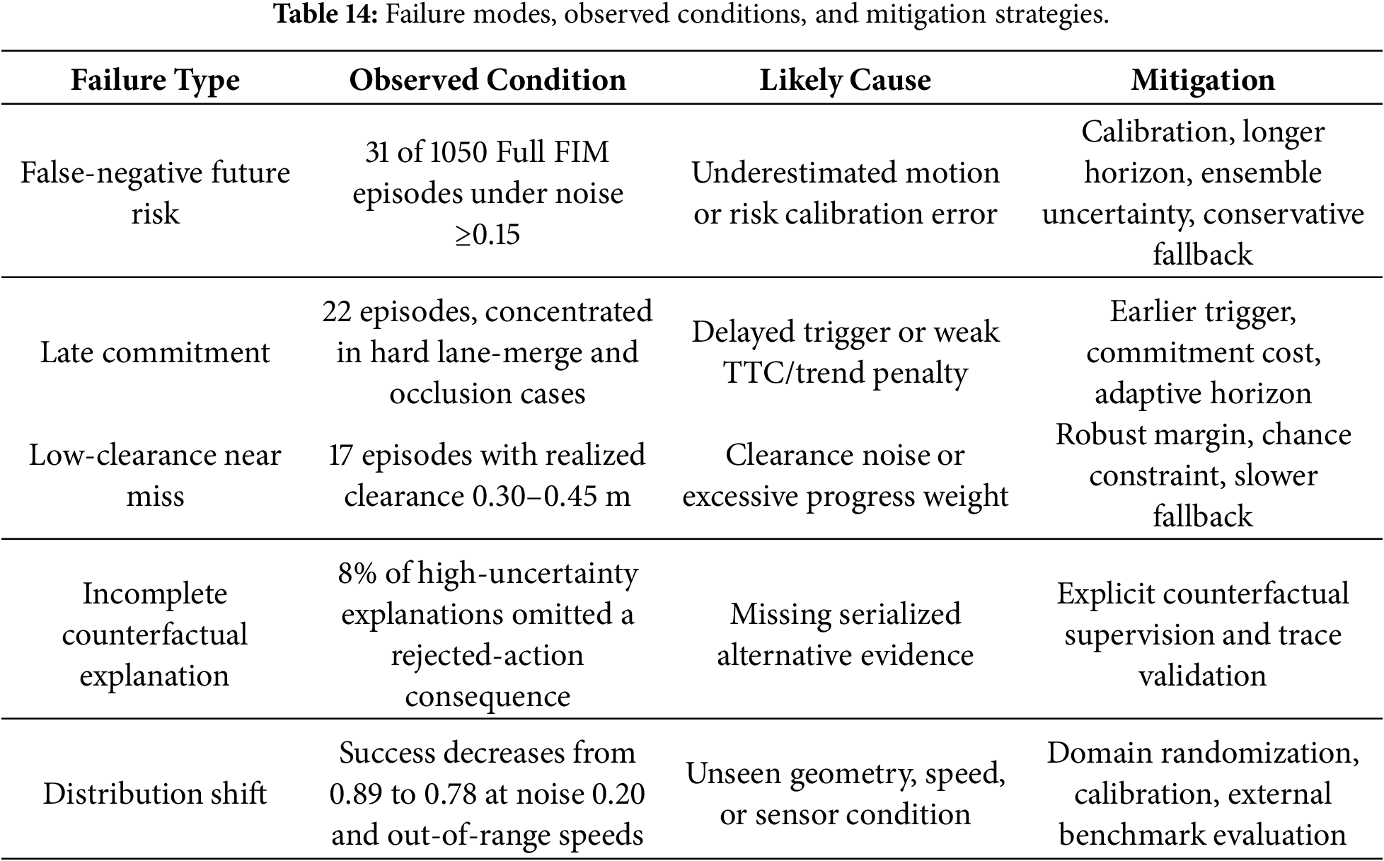
Failure analysis includes collisions, near misses, low-clearance decisions, late route commitment, false-negative future risk, route traps, and explanations missing a required counterfactual. If the full FIM has no collision in the nominal setting, stress-test or near-failure episodes are reported rather than inventing failures. Each example identifies the relevant prediction error, descriptor behavior, selected and rejected actions, and explanation limitation. Table 14 summarizes the observed failure modes, the conditions under which they occur, their likely causes, and the corresponding mitigation strategies.

9  Ethical, Practical, and Deployment Considerations

The proposed framework processes safety-critical predictions and generates explanations that may influence human trust. A plausible explanation must not be interpreted as evidence that the underlying action is correct. The explanation is therefore presented together with confidence, risk, and future-summary fields and is generated after or asynchronously from the safety decision. The language model is not authorized to override the planner.

Accountability applies to the complete pipeline rather than to the explanation module alone. An unsafe action can originate from sensor failure, biased or incomplete data, world-model error, latent misalignment, threshold calibration, action-scoring error, or inappropriate fallback behavior. Deployment requires system-level hazard analysis, redundancy, logging, independent safety monitors, and clear responsibility for configuration and updates.

Data bias and privacy also require attention. The datasets differ in geography, road infrastructure, weather, traffic culture, sensor placement, and annotation style. A model trained on these sources may perform differently for underrepresented environments or road users. Data provenance, consent, retention, and access controls should be documented, and results should be stratified where possible rather than presented as globally uniform.

Practical deployment requires bounded latency, memory use, calibration under distribution shift, and robustness to sensor degradation. Conditional FIM activation reduces average computation but creates a trigger-design trade-off: an overly conservative trigger increases latency, whereas an overly selective trigger may miss emerging risk. The reported simulation latency is hardware- and implementation-dependent and does not by itself establish compliance with an automotive real-time deadline.

10  Limitations

The expanded evaluation remains controlled and simulation-based. The original scenario uses a simplified kinematic ego proxy, discrete lane-level actions, and a safety-radius collision approximation. Even with additional scenario families, the experiments do not reproduce full vehicle dynamics, dense urban interaction, rare road-user behavior, realistic sensor artifacts, or all regulatory constraints.

FIM depends on the quality and calibration of the upstream world model. Structured interpretation cannot recover a hazard that is entirely absent from the predicted rollout. Alignment losses reduce semantic drift but do not guarantee that future latent states remain valid under substantial distribution shift. Longer horizons may improve anticipation while also increasing uncertainty and computational cost.

The decision descriptors and their thresholds encode design choices. Sensitivity analysis identifies stable regions but does not prove that one configuration is optimal across environments. The Oracle comparison is defined relative to the same candidate set and cost function; matching an Oracle under this controlled definition does not imply globally optimal driving.

Explanation grounding is evaluated primarily against structured model traces. This establishes internal consistency but not necessarily human usefulness, legal adequacy, or causal truth. A single LLM judge may be biased toward fluent text. Unless expert evaluation was completed, the manuscript explicitly states that human calibration and inter-rater reliability remain future work.

Finally, the public datasets are used for complementary component training rather than a unified closed-loop benchmark. Validation on standardized closed-loop platforms, continuous-control planners, embedded automotive hardware, and physical vehicles remains necessary before deployment claims can be made. In particular, the current study does not report CARLA, nuPlan, or other widely adopted closed-loop benchmark results; such evaluation is required before stronger claims can be made about generalization across maps, traffic densities, sensor configurations, and planner interfaces.

11  Discussion

The experiments are designed to determine whether the value of FIM comes from access to future predictions, from generic risk-aware planning, or from the structured combination of temporal, geometric, uncertainty, and semantic descriptors. Stronger current-risk, handcrafted future-risk, uncertainty-aware, MPC, and risk-aware MPC baselines provide a more demanding comparison than the original progress-only world model baseline. Descriptor ablations further reveal which variables contribute to early hazard rejection, safety margin, route commitment, and explanation grounding.

The central claim is therefore narrower and more defensible: under the evaluated controlled settings, explicitly interpreting predicted futures can improve the usability of world-model rollouts for safety-aware planning and can provide a clearer evidence trace for future-conditioned explanation. The claim is not that FIM replaces modern planners or guarantees safe autonomous driving. Instead, it offers an auditable interface that can be combined with stronger planning and prediction systems. Accordingly, the contribution should be read as evidence for an interpretable future-summary interface under controlled ambiguity, not as a complete autonomous-driving stack or a validated deployment-ready planner.

In the randomized suite, Full FIM improves success by 0.05 over risk-aware MPC (95% CI [0.02, 0.08], p = 0.003), reduces collision by 0.03 (95% CI [−0.05, −0.01], p = 0.006), improves RAA by 0.06 (95% CI [0.04, 0.08], p < 0.001), reduces DOG by 0.24 (95% CI [−0.31, −0.17], p < 0.001), and increases mean clearance by 0.07 m (95% CI [0.03, 0.11], p = 0.001). The improvement is consistent across most controlled scenario families but narrows under severe prediction noise and high-speed late-onset hazards, which limits the strength of generalization claims.

12  Conclusion

This work introduced a structured interpretation layer for predictive and explainable autonomous driving. Rather than passing latent world-model rollouts directly to downstream modules, the proposed FIM maps aligned future features into risk trend, peak risk, time-to-critical, minimum clearance, predicted collision, dominant predicted event, and confidence. These variables support a safety-aware candidate comparison and provide the evidence used to generate factual and counterfactual explanations.

The study strengthens the original evidence through aligned head reuse, explicit metric definitions, stronger planning baselines, descriptor ablations, parameter sensitivity, randomized scenario variations, statistical comparisons, latency/resource analysis, and failure-case reporting.

In the evaluation, Full FIM reaches 0.89 success and 0.05 collision, compared with 0.84 and 0.08 for the strongest non-FIM baseline, while improving RAA from 0.83 to 0.89 and reducing DOG from 0.56 to 0.32. The results support structured future interpretation as a useful complement to predictive driving models under controlled ambiguity. However, the framework remains dependent on upstream prediction quality and has not yet established full robustness under standard closed-loop real-world benchmarks. Future work will address continuous control, dense multi-agent interaction, independent evaluation on standardized closed-loop benchmarks such as CARLA and nuPlan, human-calibrated explanation assessment, deployment on automotive edge hardware, and eventual validation under physical-vehicle or hardware-in-the-loop conditions.

Acknowledgement: Not applicable.

Funding Statement: This research was funded by the Ongoing Research Funding Program, King Saud University, Riyadh, Saudi Arabia (ORF-2026-698) and ISEN Toulon Méditerranée.

Author Contributions: The authors confirm contribution to the paper as follows: Conceptualization, Rihem Farkh; methodology, Rihem Farkh; software, Rihem Farkh, Alaeddine Moussa; validation, Rihem Farkh, Ghislain Oudinet and Alaeddine Moussa; formal analysis, Rihem Farkh, Ghislain Oudinet and Alaeddine Moussa; investigation, Rihem Farkh; data curation, Rihem Farkh; writing—original draft preparation, Rihem Farkh, Ghislain Oudinet and Alaeddine Moussa; writing—review and editing, Rihem Farkh, Ghislain Oudinet, Alaeddine Moussa and Yasser Fouad; visualization, Rihem Farkh; supervision, Rihem Farkh; project administration, Rihem Farkh; funding acquisition, Ghislain Oudinet, Yasser Fouad. All authors reviewed and approved the final version of the manuscript.

Availability of Data and Materials: The data that support the findings of this study are available from the Corresponding Author, Yasser Fouad, upon reasonable request.

Ethics Approval: Not applicable; this study does not involve human participants or animals.

Conflicts of Interest: The authors declare no conflicts of interest.

Appendix A Reproducibility and Explanation-Evaluation Protocol

Appendix A.1 Qwen2.5 Judge Prompt

System role: You are an evaluator of autonomous-driving explanations. Evaluate only consistency with the provided structured context. Do not reward writing style when the explanation is not supported by the context.

Inputs: scenario, difficulty, selected action, rejected actions, current risk, risk trend, peak risk, TTC, minimum clearance, predicted collision, dominant predicted event, confidence, outcome, generated explanation, and counterfactual explanation.

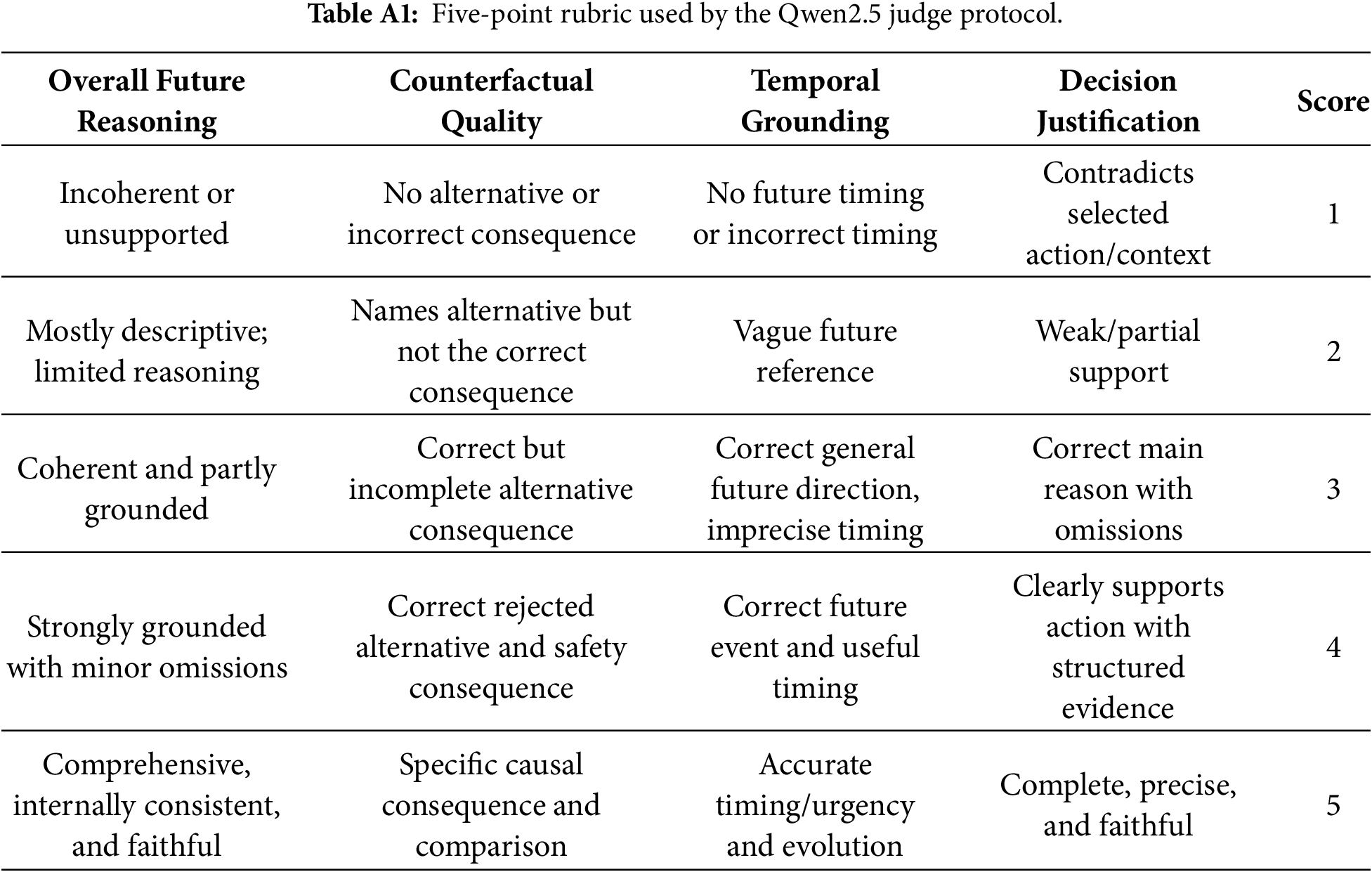
Tasks: Score decision justification, temporal grounding, counterfactual quality, and overall future reasoning from 1 to 5. For every score, return a one-sentence evidence-based justification. Do not infer objects or events not present in the structured context.

Output format: strict JSON containing the four integer scores and four justifications.

Judge settings: Qwen2.5-3B-Instruct; 4-bit quantization; temperature 0.0; top-p 1.0; maximum 512 output tokens; seeds {11, 23, 37}; three repeated judgments per explanation; median score retained.

Appendix A.2 Five-Point Rubric

Appendix A.3 Human Evaluation Statement

The LLM-based assessment is complementary and was not calibrated against human experts in this paper. The ordinal scores are therefore not interpreted as validated measures of human usefulness, legal adequacy, or trust calibration. Expert evaluation, inter-rater reliability, and comparison between human and LLM judgments remain required future work.

Appendix A.4 Reproducibility Package Statement

The reproducibility package, available upon reasonable request or with the revision materials, contains experiment configurations, selected parameters, scenario rules, per-episode summaries, metric definitions, statistical-test outputs, latency/resource measurements, the judge prompt and rubric, failure cases, and scripts used to aggregate tables and figures. External SOTA methods are marked as executed only when their original implementation, checkpoints, required datasets, and evaluation protocol were available. Otherwise, they are listed as literature comparisons or unexecuted adapters.

References

1. Kuznietsov A, Gyevnar B, Wang C, Peters S, Albrecht SV. Explainable AI for safe and trustworthy autonomous driving: a systematic review. IEEE Trans Intell Transport Syst. 2024;25(12):19342–64. doi:10.1109/tits.2024.3474469. [Google Scholar] [CrossRef]

2. Atakishiyev S, Salameh M, Yao H, Goebel R. Explainable artificial intelligence for autonomous driving: a comprehensive overview and field guide for future research directions. IEEE Access. 2024;12(3):101603–25. doi:10.1109/ACCESS.2024.3431437. [Google Scholar] [CrossRef]

3. Farkh R, Oudinet G, Deleruyelle T. Evaluating a hybrid LLM Q-learning/DQN framework for adaptive obstacle avoidance in embedded robotics. AI. 2025;6(6):115. doi:10.3390/ai6060115. [Google Scholar] [CrossRef]

4. Farkh R, Oudinet G, Adjou M, Moussa A, Fouad Y. Hybrid vision navigation with hierarchical VLM-LLM decision making. Machines. 2026;14(4):435. doi:10.3390/machines14040435. [Google Scholar] [CrossRef]

5. Mandalika S, V. L, Nambiar A. PRIMEDrive-CoT: a precognitive chain-of-thought framework for uncertainty-aware object interaction in driving scene scenario. arXiv:2504.05908. 2025. [Google Scholar]

6. Ma Y, Zhai D-H, Xia Y. CaTFormer: causal temporal transformer with dynamic contextual fusion for driving intention prediction. In: Proceedings of the 38th AAAI Conference on Artificial Intelligence; 2024 Feb 20–27; Vancouver, BC, Canada. Washington, DC, USA: AAAI Press; 2024. p. 6808–16. [Google Scholar]

7. Jia X, You J, Zhang Z, Yan J. DriveTransformer: unified transformer for scalable end-to-end autonomous driving. arXiv:2503.07656. 2025. [Google Scholar]

8. Zhu Y, Xue Y, Zhang H, Jiang G, Zhou W, Yan X, et al. DLWM: dual latent world models enable holistic Gaussian-centric pre-training in autonomous driving. arXiv:2604.00969. 2026. [Google Scholar]

9. Wang L, Zheng Y, Chen Q, Li S, Zhang Y, Xing Z, et al. Latent-WAM: latent world action modeling for end-to-end autonomous driving. arXiv:2603.24581. 2026. [Google Scholar]

10. Liu Q, Xu H, Li J, Sun B, Hao Z, She D, et al. Uni-world VLA: interleaved world modeling and planning for autonomous driving. arXiv:2603.27287. 2026. [Google Scholar]

11. Zhao L, Zhou W, Xu S, Wang C. IoT-enabled cooperative autonomous driving: a hierarchical spatial-temporal transformer framework for trajectory prediction. IEEE Internet Things J. 2026;13(8):15280–96. doi:10.1109/jiot.2026.3654101. [Google Scholar] [CrossRef]

12. You J, Chen Y, Jiang Z, Liu Z, Huang Z, Ding Y, et al. Exploring driving behavior for autonomous vehicles based on gramian angular field vision transformer. IEEE Trans Intell Transport Syst. 2024;25(11):17493–504. doi:10.1109/tits.2024.3445710. [Google Scholar] [CrossRef]

13. Gao Z, Mu Y, Chen C, Duan J, Luo P, Lu Y, et al. Enhance sample efficiency and robustness of end-to-end urban autonomous driving via semantic masked world model. IEEE Trans Intell Transport Syst. 2024;25(10):13067–79. doi:10.1109/tits.2024.3400227. [Google Scholar] [CrossRef]

14. Hafner D, Pasukonis J, Ba J, Lillicrap T. Mastering diverse domains through world models. arXiv:2301.04104v4. 2024. [Google Scholar]

15. Min C, Zhao D, Xiao L, Zhao J, Xu X, Zhu Z, et al. DriveWorld: 4D pre-trained scene understanding via world models for autonomous driving. In: Proceedings of the 2024 IEEE/CVF Conference on Computer Vision and Pattern Recognition (CVPR); 2024 Jun 16–22; Seattle, WA, USA. Piscataway, NJ, USA: IEEE; 2024. p. 15522–33. doi:10.1109/cvpr52733.2024.01470. [Google Scholar] [CrossRef]

16. Guan Y, Liao H, Li Z, Hu J, Yuan R, Zhang G, et al. World models for autonomous driving: an initial survey. IEEE Trans Intell Veh. 2025:1–17. doi:10.1109/tiv.2024.3398357. [Google Scholar] [CrossRef]

17. Zheng Y, Yang P, Xing Z, Zhang Q, Zheng Y, Gao Y, et al. World4Drive: end-to-end autonomous driving via intention-aware physical latent world model. In: Proceedings of the 2025 IEEE/CVF International Conference on Computer Vision (ICCV); 2025 Oct 19–25; Honolulu, HI, USA. Piscataway, NJ, USA: IEEE; 2025. p. 28632–42. doi:10.1109/iccv51701.2025.02659. [Google Scholar] [CrossRef]

18. Wang X, Zhu Z, Huang G, Chen X, Zhu J, Lu J. DriveDreamer: towards real-world-driven world models for autonomous driving. In: Computer Vision–ECCV 2024. Cham, Switzerland: Springer; 2024. p. 55–72. [Google Scholar]

19. Zhao G, Wang X, Zhu Z, Chen X, Huang G, Bao X, et al. DriveDreamer-2: LLM-enhanced world models for diverse driving video generation. arXiv:2403.06845. 2024. [Google Scholar]

20. Blackmore L, Ono M, Williams BC. Chance-constrained optimal path planning with obstacles. IEEE Trans Robot. 2011;27(6):1080–94. doi:10.1109/TRO.2011.2161160. [Google Scholar] [CrossRef]

21. Mayne DQ. Model predictive control: recent developments and future promise. Automatica. 2014;50(12):2967–86. doi:10.1016/j.automatica.2014.10.128. [Google Scholar] [CrossRef]

22. Schulman J, Ho J, Lee A, Awwal I, Bradlow H, Abbeel P. Finding locally optimal, collision-free trajectories with sequential convex optimization. In: Robotics: science and systems IX. Stanford, CA, USA: Robotics: Science and Systems Foundation; 2013. doi:10.15607/rss.2013.ix.031. [Google Scholar] [CrossRef]

23. Hayward JC. Near-miss determination through use of a scale of danger. Highway Res Rec. 1972;384:24–34. [Google Scholar]

24. Hu Y, Yang J, Chen L, Li K, Sima C, Zhu X, et al. Planning-oriented autonomous driving. In: Proceedings of the 2023 IEEE/CVF Conference on Computer Vision and Pattern Recognition (CVPR); 2023 Jun 17–24; Vancouver, BC, Canada. Piscataway, NJ, USA: IEEE; 2023. p. 17853–62. doi:10.1109/cvpr52729.2023.01712. [Google Scholar] [CrossRef]

25. Jiang B, Chen S, Xu Q, Liao B, Chen J, Zhou H, et al. VAD: vectorized scene representation for efficient autonomous driving. In: Proceedings of the 2023 IEEE/CVF International Conference on Computer Vision (ICCV); 2023 Oct 1–6; Paris, France. Piscataway, NJ, USA: IEEE; 2023. p. 8306–16. doi:10.1109/iccv51070.2023.00766. [Google Scholar] [CrossRef]

26. Sima C, Renz K, Chitta K, Chen L, Zhang H, Xie C, et al. DriveLM: driving with graph visual question answering. In: Computer Vision—ECCV 2024 (ECCV 2024). Cham, Switzerland: Springer; 2024. p. 256–74. [Google Scholar]

27. Tian X, Gu J, Li B, Liu Y, Wang Y, Zhao Z, et al. DriveVLM: the convergence of autonomous driving and large vision-language models. arXiv:2402.12289. 2024. [Google Scholar]

28. Mandalika S, Nambiar A. SegXAL: explainable active learning for semantic segmentation in driving scene scenarios. In: Pattern recognition. Cham, Switzerland: Springer Nature; 2025. p. 117–34. doi:10.1007/978-3-031-78107-0_8. [Google Scholar] [CrossRef]

29. Kolekar S, Gite S, Pradhan B, Alamri A. Explainable AI in scene understanding for autonomous vehicles in unstructured traffic environments on Indian roads using the inception U-Net model with grad-CAM visualization. Sensors. 2022;22(24):9677. doi:10.3390/s22249677. [Google Scholar] [CrossRef]

30. Nie M, Peng R, Wang C, Cai X, Han J, Xu H, et al. Reason2Drive: towards interpretable and chain-based reasoning for autonomous driving. In: Computer Vision—ECCV 2024. Cham, Switzerland: Springer Nature; 2025. p. 292–308. doi:10.1007/978-3-031-73347-5_17. [Google Scholar] [CrossRef]

31. Chang CP, Wang CY, Caesar H, Pagani A. Probing the reliability of driving VLMs: from inconsistent responses to grounded temporal reasoning. arXiv:2603.09512. 2026. [Google Scholar]

32. Feng Y, Feng Z, Hua W, Sun Y. Multimodal-XAD: explainable autonomous driving based on multimodal environment descriptions. IEEE Trans Intell Transp Syst. 2024;25(12):19469–81. doi:10.1109/tits.2024.3467175. [Google Scholar] [CrossRef]

33. Pan B, Sun J, Leung HYT, Andonian A, Zhou B. Cross-view semantic segmentation for sensing surroundings. IEEE Robot Autom Lett. 2020;5(3):4867–73. doi:10.1109/LRA.2020.3004325. [Google Scholar] [CrossRef]

34. Zhou B, Krahenbuhl P. Cross-view transformers for real-time map-view semantic segmentation. In: Proceedings of the 2022 IEEE/CVF Conference on Computer Vision and Pattern Recognition (CVPR); 2022 Jun 19–24; New Orleans, LA, USA. Piscataway, NJ, USA: IEEE; 2022. p. 13750–9. [Google Scholar]

35. Zeng S, Chang X, Xie M, Liu X, Bai Y, Pan Z, et al. FutureSightDrive: thinking visually with spatio-temporal CoT for autonomous driving. arXiv:2505.17685. 2025. [Google Scholar]

36. Azarafza M, Nayyeri M, Steinmetz C, Staab S, Rettberg A. Hybrid reasoning based on large language models for autonomous car driving. In: Proceedings of the 2024 12th International Conference on Control, Mechatronics and Automation (ICCMA); 2024 Nov 11–13; London, UK. Piscataway, NJ, USA: IEEE; 2024. p. 14–22. doi:10.1109/ICCMA63715.2024.10843921. [Google Scholar] [CrossRef]

37. Xu Z, Zhang Y, Xie E, Zhao Z, Guo Y, Wong KK, et al. DriveGPT4: interpretable end-to-end autonomous driving via large language model. arXiv:2310.01412. 2023. [Google Scholar]

38. Kalapos A, Gór C, Moni R, Harmati I. Sim-to-real reinforcement learning applied to end-to-end vehicle control. In: Proceedings of the 2020 23rd International Symposium on Measurement and Control in Robotics (ISMCR); 2020 Oct 15–17; Budapest, Hungary. Piscataway, NJ, USA: IEEE; 2020. p. 1–6. doi:10.1109/ISMCR51255.2020.9263751. [Google Scholar] [CrossRef]

39. Kaushik R, Arndt K, Kyrki V. SafeAPT: safe simulation-to-real robot learning using diverse policies learned in simulation. IEEE Robot Autom Lett. 2022;7(3):6838–45. doi:10.1109/LRA.2022.3177294. [Google Scholar] [CrossRef]

40. Albarella N, Lui DG, Petrillo A, Santini S. A hybrid deep reinforcement learning and optimal control architecture for autonomous highway driving. Energies. 2023;16(8):3490. doi:10.3390/en16083490. [Google Scholar] [CrossRef]

41. Lei N, Zhang H, Hu J, Hu Z, Wang Z. Sim-to-real design and development of reinforcement learning-based energy management strategies for fuel cell electric vehicles. Appl Energy. 2025;393:126030. doi:10.1016/j.apenergy.2025.126030. [Google Scholar] [CrossRef]