Disturbed Dynamic Analysis and Robust Decision-Making Control of Complex Networks

1  Introduction

Complex networks arise in power grids, transportation systems, industrial Internet-of-Things platforms, communication infrastructures, and cooperative robots. Their control is difficult because interactions are sparse and heterogeneous, topology information can change, disturbances are only partially observed, and the available intervention budget is usually much smaller than the network size. Small-world structure remains a useful reproducible model for local interaction and long-range shortcuts [1], while data-driven network control and structural controllability provide principled tools for selecting informative actuation channels [2,3].

Robust data-driven feedback design can convert noisy trajectories into certified controllers [4], and recent learning-based control studies exploit graph structure or side information to improve adaptation [5,6]. Complementary controllability-aware studies address sparse actuation and structural control configuration in large-scale networks [7–10], but they do not couple online disturbance estimation, dynamic actuator reallocation, and a robust safety projection. Broader network-decision research studies edge/cloud architectures and offloading [11–13], game-theoretic resource allocation [14,15], and learning-based scheduling [16,17]. Two CMC studies are retained for directly related perspectives on multi-agent formation control and AI-enabled traffic management in networked systems [18,19]. These works motivate online network decisions, but their objectives are latency, energy, or network-level performance rather than closed-loop state safety. Control-oriented surveys are closer to the present problem [20]; surveys on task-oriented mobile networks clarify the deployment context [21], but do not provide disturbance-certified actuator allocation. However, three gaps remain. First, a learned predictor and the estimator analyzed in the theory must be identical. Second, safety-filter feasibility cannot be left as an unqualified assumption, especially after abrupt topology changes. Third, sparse network-control studies often report only synthetic, single-run averages without statistical variability, real benchmark topology, or large-scale timing.

Recent resilient control provides useful complementary perspectives. Robust distributed MPC explicitly handles disturbances and denial-of-service interruptions [22], whereas resilient fuzzy adaptive control addresses input constraints, nonlinear uncertainty, and false-data injection in multi-agent systems [23]. These methods focus on fixed agent-level control protocols or distributed prediction under specified attack models. R-D3C instead addresses the joint online problem of identifying changing network dynamics, estimating an uncertainty envelope, reallocating a limited actuator set, and certifying the final action. The distinction is important: robust MPC alone does not decide which nodes should be actuated, and a graph policy alone does not certify the applied input.

The proposed R-D3C framework uses a graph-regularized sliding window to estimate local dynamics and residual energy. A disturbance-sensitive score then combines state risk, local disagreement, topology, and recent residuals. A greedy budgeted allocator chooses the active nodes, a receding-horizon policy generates a nominal command, and a robust projection verifies the Lyapunov decrease. If the strict constraint is infeasible, a penalized slack problem and a saturated backup action are invoked; the paper clearly distinguishes strict certification from best-effort fallback operation.

The contributions are summarized as follows. (1) We formulate a unified identification–allocation–control problem in which the actuator set changes with the measured disturbance path. (2) We derive practical stability and sparse risk-reduction guarantees and establish a dynamic-regret bound for the exact sliding-window ridge estimator used in the algorithm and experiments. (3) We provide a verifiable safety-feasibility condition, radius inflation after topology changes, and an explicit fallback. (4) We report reproducible baseline settings, a 30-paired-run nominal comparison with significance tests, a separate 20-run deployment-impairment benchmark, an IEEE 39-bus topology experiment [24], and runtime scaling to 1000 nodes.

The remainder of this paper is organized as follows. Section 2 defines the disturbed network problem. Section 3 develops identification and robust-set construction. Section 4 presents R-D3C. Section 5 gives the theoretical analysis. Section 6 reports the experiments, and Section 7 concludes the paper.

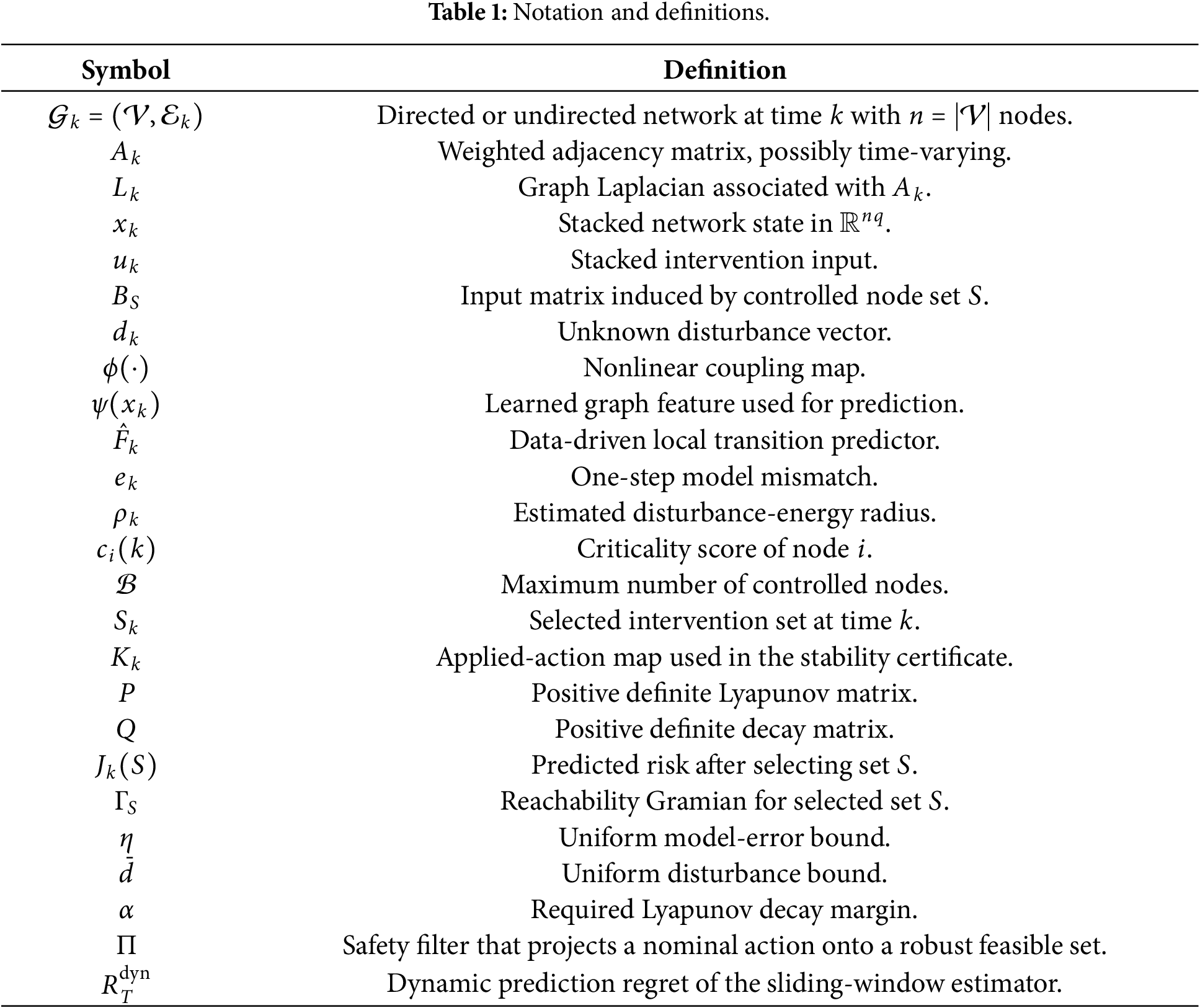
Table 1 summarizes the principal notation used throughout the manuscript.

2  Problem Description and Preliminaries

2.1 Disturbed Network Dynamics

Consider a network with n nodes. Node i has state xi(k)∈Rq. The local dynamics are written as

xi(k+1)=fi(xi(k))+∑j=1naij(k)ϕij(xj(k)−xi(k))+biui(k)+di(k),(1)

where aij(k) is the coupling weight, ui(k) is a control input, and di(k) is an unknown disturbance. Stacking all node states gives

xk+1=Fk(xk)+BSuk+dk,(2)

where S⊆𝒱 is the set of controlled nodes. Only |S|≤ℬ nodes may be controlled. The controller receives node measurements, partial graph data, and resource limits. The goal is to choose Sk and uk so that xk approaches a safe target set while control cost remains low.

The disturbed network is not assumed to be exactly known. The adjacency matrix can switch slowly, and the coupling functions can include unmodeled nonlinear terms. We therefore use a local data-driven approximation

xk+1=F^kxk+H^kψ(xk)+BSkuk+ek+dk,(3)

where ψ(xk) collects graph features such as local disagreement, degree-normalized state, and neighbor residuals. The model mismatch satisfies ‖ek‖≤ηk‖xk‖+ξk. The disturbance satisfies ‖dk‖≤ρk with an estimated envelope ρk.

2.2 Risk and Decision Variables

Let 𝒳s={x:xTPx≤rs2} be the safe region. We define the instantaneous risk as

ℛ(xk,Sk,uk)=xk+1TPxk+1+λu‖uk‖22+λb|Sk|,(4)

where P≻0 and λu,λb>0. The decision problem is

minSk,ukℛ(xk,Sk,uk)s.t.|Sk|≤ℬ,‖uk‖∞≤umax,(x^k+1+w)TP(x^k+1+w)−xkTPxk≤−α‖xk‖2+σ,∀w: ‖w‖≤ηk‖xk‖+ξk+ρk.(5)

This problem joins three tasks: dynamic prediction, node-set selection, and robust input synthesis. The set constraint is combinatorial. The safety inequality is robust against both prediction error and disturbance.

Fig. 1 makes the information dependencies explicit: only measured transitions enter the estimator, the disturbance envelope affects both allocation and projection, and the applied transition is returned to the next window. This prevents the learned ranking module from bypassing the safety layer.

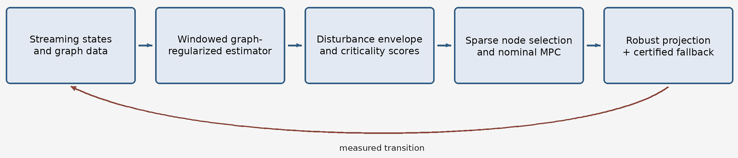
Figure 1: Closed-loop information and control flow of R-D3C.

2.3 Preliminaries

For a fixed set S, define the local closed-loop matrix

MS,k=F^k+H^k∂ψ∂x(xk)−BSKk.(6)

For the stability certificate of Section 5.1, the matrix test is tied to the action actually applied. For every zero-slack applied action with xk≠0, define the one-step action-equivalent map Kkapp=−ukxkT/(xkTxk), which satisfies uk=−Kkappxk at the current state. For xk=0, certification requires the zero action and uses Kkapp=0. The matrix condition in Assumption 5.2 is checked with this action-equivalent map; hence no assumption is made that a constrained or nonlinear MPC command is generated by a fixed linear feedback gain. The Riccati recursion is used only to warm-start the nominal optimizer. The Jacobian in Eq. (6) is evaluated at differentiability points of the chosen feature map; this local differentiability is needed to form the linearization, whereas no separate global Lipschitz constant for ψ is required by the present proofs.

The h-step reachability Gramian is

ΓS(h)=∑ℓ=0h−1MS,kℓBSBST(MS,kT)ℓ.(7)

A set with a larger minimum eigenvalue of ΓS(h) can influence more network directions. We also define the local criticality score

ci(k)=ω1∂r^k∂xiPi∂r^k∂xiT+ω2degi(k)+ω3Δ^i(k),(8)

where r^k is predicted risk, degi is normalized degree, and Δ^i estimates local disturbance amplification. The score is not a pure centrality measure. It is a control-oriented quantity that changes with the current state and disturbance estimate.

Remark 1: The formulation differs from static pinning control. A fixed pinning set can be effective when the topology and disturbance channels are stable. Here, the selected set is allowed to change because the most useful intervention nodes may shift after disturbances, load changes, or topology drift. The robust constraint prevents these changes from sacrificing stability.

3  Model and Analysis

3.1 Graph-Regularized Dynamic Identification

The predictor is updated from a sliding data window

𝒟k={xt,ut,xt+1,At}t=k−mk−1.(9)

Let Θk=[F^k,H^k] and φt=[xtT,ψ(xt)T]T. We solve

Θk=arg⁡minΘ∑t=k−mk−1‖xt+1−Θφt−BStut‖22+λgtr⁡(ΘℒfΘT)+λr‖Θ‖F2,(10)

where ℒf is a feature graph Laplacian. The term tr⁡(ΘℒfΘT) encourages nearby graph features to have similar dynamic effects. This regularization is useful when several nodes have sparse observations. To make the estimator explicit, define

Φk=[φk−m,…,φk−1],Yk=[yk−m,…,yk−1],yt=xt+1−BStut.(11)

The first-order optimality condition of (10) is

Θk(ΦkΦkT+λgℒf+λrI)=YkΦkT.(12)

Hence, if the regularized information matrix is nonsingular, the estimator has the closed form

Θk=YkΦkT(ΦkΦkT+λgℒf+λrI)−1.(13)

The local information level is quantified as

ιk=λmin(ΦkΦkT+λgℒf+λrI),(14)

which controls the sensitivity of the estimator to measurement noise. A larger ιk yields a smaller parameter deviation bound

‖Θk−Θk⋆‖F≤‖EkΦkT‖Fιk,(15)

where Ek stacks one-step residual disturbances in the data window. This bound explains why graph regularization is useful when the raw trajectory matrix is poorly conditioned.

The residual sequence is

ϵt=xt+1−Θkφt−BStut.(16)

We estimate the disturbance radius by

ρk=1m∑t=k−mk−1‖ϵt‖22+τmaxt∈[k−m,k−1]‖ϵt‖2,(17)

where τ∈[0,1] controls conservatism. The radius captures both persistent noise and rare shocks. To reduce underestimation immediately after a topology change, the implemented envelope is ρ~k=max{ρk,ρk−1}+δA‖Ak−Ak−1‖F, where δA is calibrated from validation trajectories; the oldest window is discarded and the inflated radius is retained for mr steps. The resulting envelope is inserted into the robust safety filter.

3.2 Disturbance Amplification and Critical Transition

Let V(x)=xTPx. Using (3), the worst-case one-step Lyapunov growth under set S and gain K satisfies

ΔVk≤xkT(MS,kTPMS,k−P)xk+2‖MS,kTPxk‖w¯k+λmax(P)w¯k2,(18)

where w¯k=ηk‖xk‖+ξk+ρk. A critical transition occurs when the positive disturbance terms exceed the nominal decay. Thus, a useful intervention set must reduce the first term and shrink the multiplier of w¯k.

Fig. 2 is generated from numerical trials rather than a conceptual node sketch. A trial is counted as successful when its terminal residual RMS is below 0.065 and its violation rate is below 3%; each cell averages ten seeds. The boundary shows how stronger disturbances require a larger intervention budget.

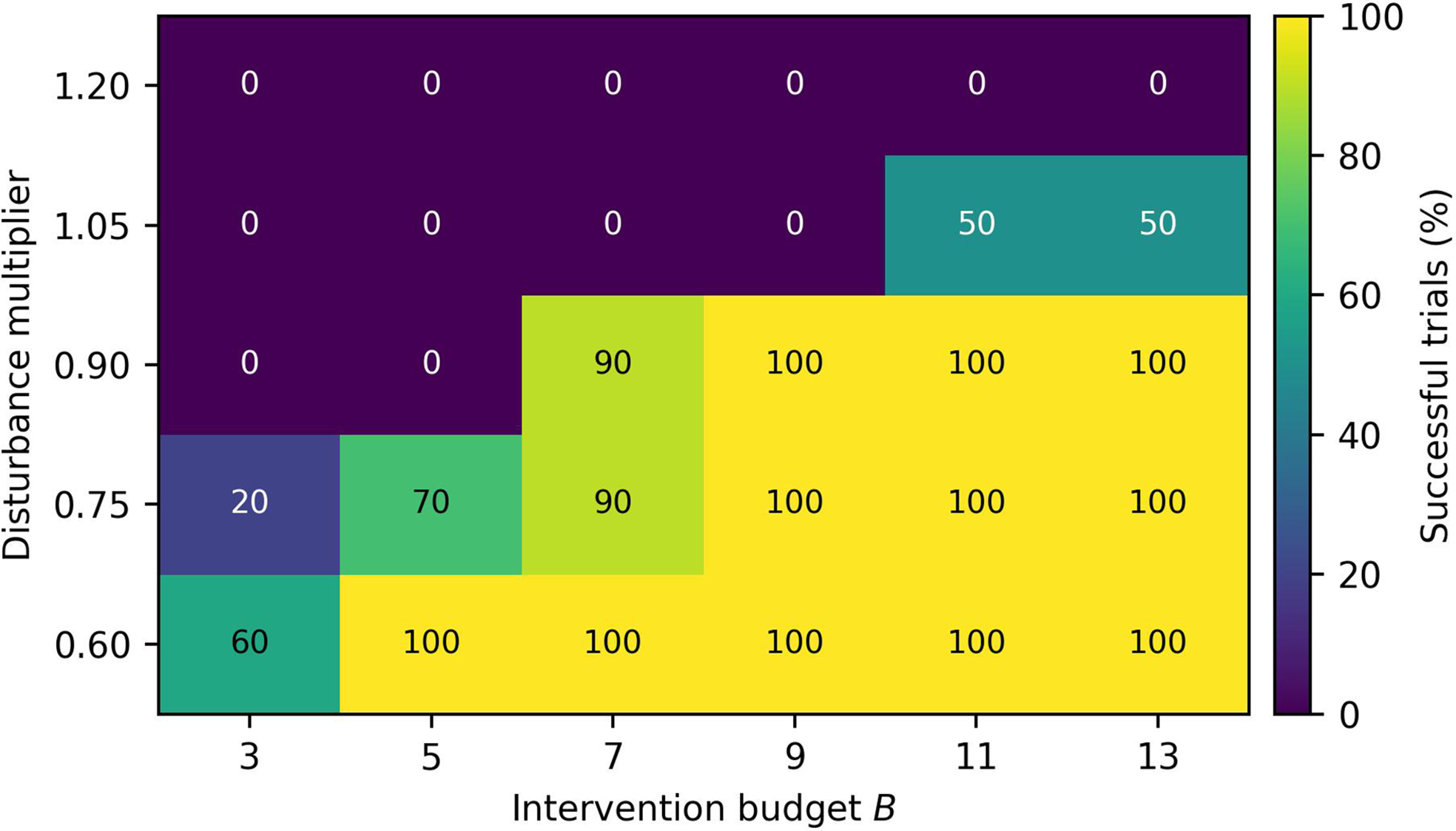
Figure 2: Measured stabilization success vs. disturbance level and intervention budget.

3.3 Robust Safe Set

The robust one-step feasible set is

𝒞k={u: sup‖w‖≤w¯k[(x^k+1+w)TP(x^k+1+w)−xkTPxk]≤−α‖xk‖2+σ}.(19)

The inner supremum in (19) admits the support-function upper expression

sup‖w‖≤w¯k(x^k+1+w)TP(x^k+1+w)≤x^k+1TPx^k+1+2w¯k‖Px^k+1‖+λmax(P)w¯k2.(20)

Therefore, define the safety margin

mk(u)=−α‖xk‖2+σ−x^k+1TPx^k+1−2w¯k‖Px^k+1‖−λmax(P)w¯k2.(21)

The robust feasible set can equivalently be approximated by the convex inequality

𝒞k={u: mk(u)≥−xkTPxk, ‖u‖∞≤umax}.(22)

With the corrected signs in Eq. (21), the condition mk(u)≥−xkTPxk is exactly the conservative upper-bound form of Eq. (19): it implies the worst-case decrease ΔVk≤−α‖xk‖2+σ.

A nominal input uk0 is projected onto this set:

uk=Π𝒞k(uk0)=arg⁡minu∈𝒞k‖u−uk0‖22.(23)

A checkable sufficient condition for 𝒞k≠∅ is the existence of a backup gain Kb satisfying

MbTPMb−P⪯−Qb,‖Kbxk‖∞≤umax,(24)

and

(λmin(Qb)−α)‖xk‖2≥2‖MbTPxk‖w¯k+λmax(P)w¯k2−σ,λmin(Qb)>α,(25)

where Mb is the local closed-loop matrix under u=−Kbx. The −α term in Eq. (25), together with Eq. (24), makes the backup condition sufficient for the same zero-slack inequality in Eq. (19). Conditions (24), (25) are evaluated online. If they fail or the strict projection is infeasible, R-D3C solves

minu,s≥0 ‖u−uk0‖22+κss2s.t.mk(u)+xkTPxk+s≥0,(26)

then activates an emergency reserve ℬe=min{n,ℬ+2} and applies the saturated backup input. A zero slack retains the strict certificate; positive slack is explicitly logged as best-effort operation and does not inherit the strict Lyapunov guarantee.

The projection is well posed because 𝒞k is closed and convex after the cone approximation. Its nonexpansive property gives

‖Π𝒞k(a)−Π𝒞k(b)‖2≤‖a−b‖2,(27)

which prevents a noisy nominal policy from being amplified by the safety layer. The projection can be solved as a second-order cone program because (20) is conic representable. When computational resources are limited, a diagonal P and local input constraints yield a separable approximation.

Fig. 3 clarifies the projection geometry. The nominal successor can lie inside the disturbance-expanded boundary but outside the contracted safe set; projection moves it toward a certified successor whenever the strict constraints are feasible.

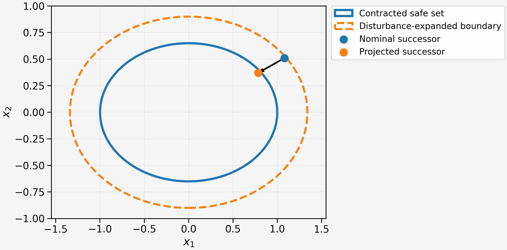
Figure 3: Nominal and projected successors relative to robust safe regions.

Remark 2: The analysis separates prediction and certification. The predictor improves performance by estimating the current dynamic trend, but the robust set is the object that protects the closed loop. This design is important when machine learning is used in safety-sensitive networks because a low training error does not imply stable closed-loop behavior.

4  Algorithm Design

4.1 Design Motivation

The proposed algorithm is called R-D3C, namely robust disturbance-aware data-driven decision control. A disturbed network needs rapid intervention, but the controller cannot actuate all nodes. The controller must decide which nodes are important, how strong the disturbance is, and which feasible action reduces risk without violating safety.

R-D3C uses four coupled modules. The first module updates the graph-regularized predictor (10). The second module estimates the disturbance envelope (17). The third module computes node criticality (8) and selects a sparse intervention set. The fourth module computes a nominal action and then projects it onto (19). The algorithmic idea is to use learning for ranking and prediction, but use robust optimization for the final decision.

4.2 Sparse Robust Allocation

The exact set-selection problem is NP-hard because it contains a cardinality constraint. We use a submodular surrogate. Define

J^k(S)=tr⁡(P(I+ΓS(h))−1)+λb|S|−λc∑i∈Sci(k).(28)

The first term rewards controllability, the second term penalizes intervention cost, and the last term rewards disturbance-sensitive nodes. Starting from S=∅, the algorithm adds the node with the largest marginal decrease in J^k(S) until |S|=ℬ or no positive decrease remains:

i∗=argmaxi∉S[J^k(S)−J^k(S∪{i})].(29)

This rule is lightweight and can be implemented in parallel because marginal gains depend on local criticality and low-rank Gramian updates.

Table 2 summarizes the complete R-D3C procedure, including the feasibility fallback.

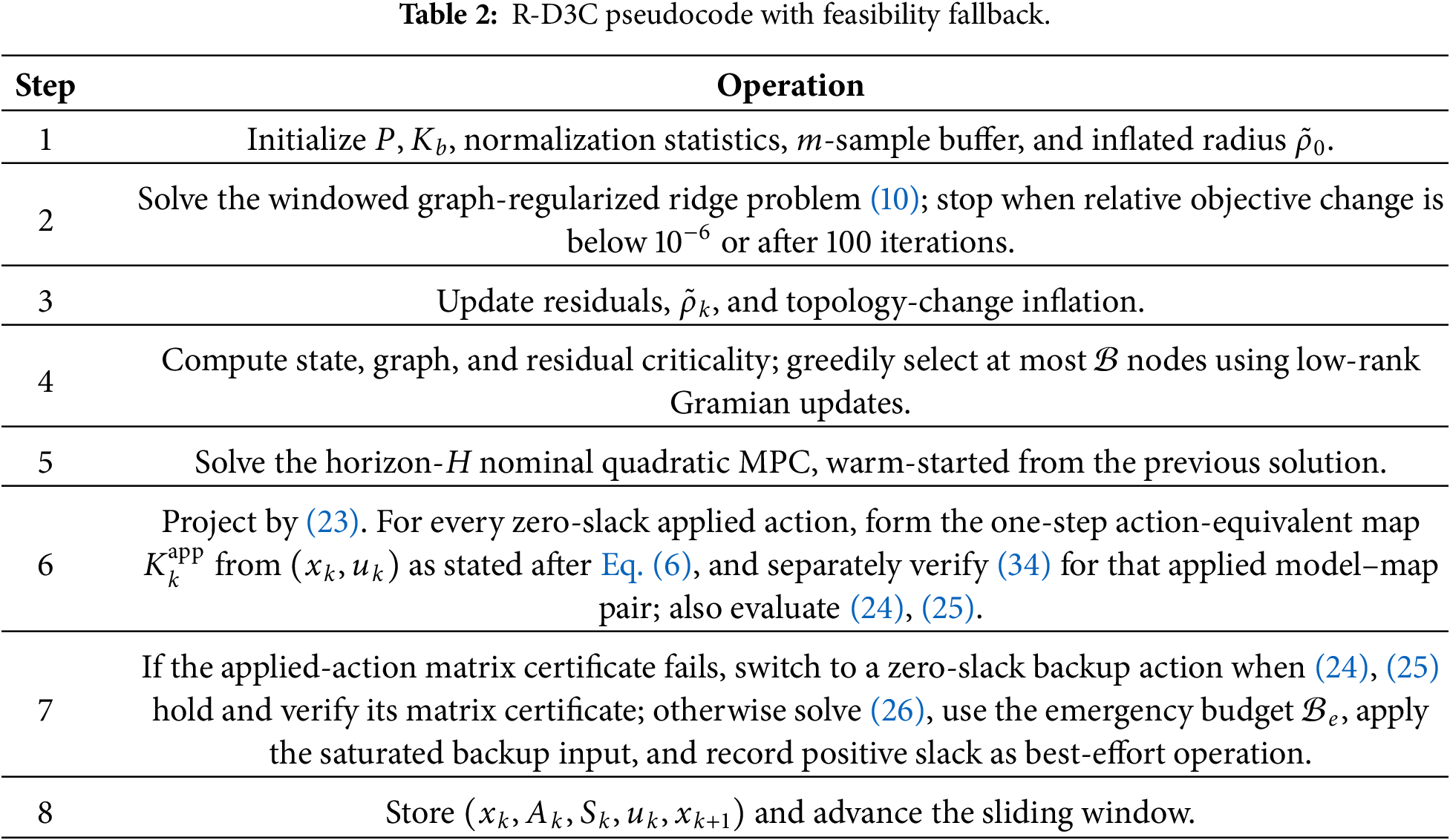
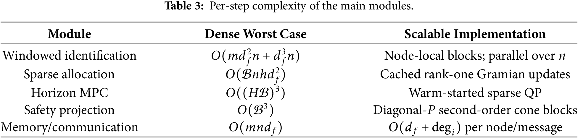
Table 3 reports the per-step computational complexity of the main modules.

4.3 Nominal Receding-Horizon Policy

For a selected set Sk, the nominal policy solves

minuk:k+H−1∑ℓ=0H−1(x^k+ℓTPx^k+ℓ+λu‖uk+ℓ‖22)+x^k+HTPfx^k+Hs.t.x^k+ℓ+1=F^kx^k+ℓ+H^kψ(x^k+ℓ)+BSkuk+ℓ,‖uk+ℓ‖∞≤umax.(30)

Only the first input is used. The safety filter then checks this input against the worst-case inequality. In practice, the nominal policy may be a quadratic MPC, a neural warm-start, or a linear feedback uk0=−Kkxk. For the linearized local predictor, the backward recursion

Pℓ=P+MSk,kTPℓ+1MSk,k−MSk,kTPℓ+1BSkΛℓ−1BSkTPℓ+1MSk,k(31)

with

Λℓ=λuI+BSkTPℓ+1BSk,(32)

produces the warm-start gain

Kℓ=Λℓ−1BSkTPℓ+1MSk,k.(33)

The final action is still the projected action in (23).

Remark 3: R-D3C is not a black-box reinforcement-learning controller. Learning estimates the local model and ranks the nodes, but the deployed control is obtained after a stability-oriented projection. This structure allows data-driven adaptation while keeping the stability proof independent of the exact neural or regression architecture used for prediction.

5  Algorithm Analysis

5.1 Practical Stability

Assumption 1: The combined model error and exogenous disturbance are uniformly bounded on the operating region by ‖wk‖≤w¯k=η‖xk‖+ξ¯+d¯.

No separate global Lipschitz constant for ψ is required by the stability or regret analysis; only the local differentiability stated after Eq. (6) is invoked to form the linearization.

Assumption 2: For each action claimed as certified zero-slack operation, Kkapp is the one-step action-equivalent map constructed from the actually applied pair (xk,uk), so that uk=−Kkappxk on that step. Using Kkapp in Eq. (6), the resulting applied closed-loop matrix MSk,kapp must satisfy the separately checked standing condition

(MSk,kapp)TPMSk,kapp−P⪯−Q,P≻0, Q≻0.(34)

This matrix certificate is not inferred from scalar membership in 𝒞k or from the projection in (23). A nominal MPC step is covered by Theorem 1 only if the projection returns zero slack and Eq. (34) is verified for the action-equivalent map of the applied post-projection input. The same construction is used whether or not the projection changes the nominal command, so the certification does not assume that constrained MPC admits a fixed linear feedback representation. If this matrix check fails, the step is not labeled nominally certified; R-D3C switches to the backup action when Eqs. (24), (25) hold and the corresponding matrix certificate is verified. Positive-slack fallback remains best-effort and is outside the theorem.

In practice, P and Kb are obtained offline from a polytopic set of identified models by minimizing tr⁡(P) subject to (24). The decay parameter is chosen as 0<α≤λmin(Q)/(2λmax(P)); a larger α accelerates contraction but reduces feasibility. Disturbance bounds are calibrated from an upper residual quantile and inflated after graph changes, so underestimated uncertainty is visible through nonzero slack rather than being hidden. When the backup gain Kb satisfies (24), (25) and its applied matrix also satisfies Assumption 2, the zero-slack backup step is covered by the same Lyapunov argument. Positive-slack fallback intervals are deliberately excluded from Theorem 1; they are reported only as bounded-input best-effort operation.

Theorem 1 (Robust practical stability): Consider any closed-loop interval on which every applied action has zero slack and satisfies the applied-action matrix certificate in Assumption 2. Under Assumptions 1 and 2, suppose that κM=supk‖(MSk,kapp)TP‖ is finite and

μs=λQ−2κMη−λPη2>0,(35)

where λQ=λmin(Q) and λP=λmax(P). Then the closed-loop state generated by R-D3C on that certified interval is practically input-to-state stable. More precisely,

V(xk+1)−V(xk)≤−μs2‖xk‖2+χs,(36)

where w¯0=ξ¯+d¯ and

χs=[(2κM+2λPη)22μs+λP]w¯02.(37)

Consequently, every trajectory segment that remains under certified zero-slack operation enters

Ωs={x:‖x‖2≤2χsμs},(38)

and remains bounded while the certified conditions continue to hold. The theorem does not assert practical input-to-state stability across positive-slack fallback episodes.

Proof. Let x^k+1=MSk,kappxk denote the certified local-model successor under the actually applied zero-slack action, and let wk be the total error caused by model mismatch and exogenous disturbance. Then

xk+1=MSk,kappxk+wk,‖wk‖≤η‖xk‖+w¯0.(39)

Using V(x)=xTPx, we obtain

V(xk+1)−V(xk)=xkT((MSk,kapp)TPMSk,kapp−P)xk+2xkT(MSk,kapp)TPwk+wkTPwk.(40)

By Assumption 2,

xkT((MSk,kapp)TPMSk,kapp−P)xk≤−λQ‖xk‖2.(41)

The cross term and quadratic disturbance term satisfy

2xkT(MSk,kapp)TPwk≤2κMη‖xk‖2+2κMw¯0‖xk‖,(42)

wkTPwk≤λPη2‖xk‖2+2λPηw¯0‖xk‖+λPw¯02.(43)

Substituting (41)–(43) into (40) yields

ΔVk≤−μs‖xk‖2+(2κM+2λPη)w¯0‖xk‖+λPw¯02.(44)

Young’s inequality gives

(2κM+2λPη)w¯0‖xk‖≤μs2‖xk‖2+(2κM+2λPη)22μsw¯02.(45)

Combining (44) and (45) proves (36). If ‖xk‖2>2χs/μs, then V(xk+1)<V(xk). Since λmin(P)‖x‖2≤V(x)≤λmax(P)‖x‖2, the sublevel set associated with Ωs is compact. Thus, on any interval for which the certified zero-slack conditions continue to hold, the trajectory reaches the associated compact sublevel set in finite time and remains bounded on that interval. ◻

5.2 Risk Reduction of Sparse Allocation

Lemma 1: If the surrogate (28) is normalized, monotone decreasing, and has submodularity ratio γs∈(0,1], the greedy allocation satisfies

J^k(Sk)−J^k(Sk∗)≤(1−γsℬ)ℬ[J^k(∅)−J^k(Sk∗)],(46)

where Sk∗ is the best budget-feasible set.

Proof. Let Sr be the greedy set after r additions. By the definition of submodularity ratio, at least one remaining element in Sk∗∖Sr has marginal decrease no smaller than

γsℬ[J^k(Sr)−J^k(Sk∗)].(47)

The greedy choice has at least this decrease. Hence,

J^k(Sr+1)−J^k(Sk∗)≤(1−γsℬ)[J^k(Sr)−J^k(Sk∗)].(48)

Iterating from r=0 to ℬ−1 gives (46). ◻

Theorem 2 (Monotone risk improvement). Assume the prediction error of J^k(S) is bounded by εJ, namely |Jk(S)−J^k(S)|≤εJ for every feasible set. Then the set selected by R-D3C satisfies

Jk(Sk)≤Jk(∅)−(1−e−γs)[Jk(∅)−Jk(Sk∗)]+4εJ.(49)

Thus, when the learned set-value error is small, the allocation yields a guaranteed fraction of the best achievable risk decrease.

Proof. From Lemma 1 and (1−γs/ℬ)ℬ≤e−γs, we obtain

J^k(Sk)≤J^k(∅)−(1−e−γs)[J^k(∅)−J^k(Sk∗)].(50)

Using |Jk(S)−J^k(S)|≤εJ for Sk, Sk∗, and ∅ gives

Jk(Sk)≤J^k(Sk)+εJ,(51)

and

J^k(∅)−J^k(Sk∗)≥Jk(∅)−Jk(Sk∗)−2εJ.(52)

Combining the two inequalities and using (1−e−γs)≤1 and collecting the error terms into a conservative 4εJ term yields (49). The bound is conservative but explicit. ◻

5.3 Prediction Regret of the Implemented Sliding Window

Let L¯k(Θ) denote the expected one-step regularized prediction loss at time k, and let Lk(m)(Θ) be its empirical counterpart constructed from the most recent m samples in (10). Define Θk∗=arg⁡minΘL¯k(Θ) and the path variation VT=∑k=2T‖Θk∗−Θk−1∗‖F.

The constants used below can be tied directly to the implemented estimator in (10). Because ℒf⪰0 and λr>0, the ridge term makes the objective strongly convex in Θ; with the present quadratic convention, a conservative modulus is μ≥2λr (and informative data or a positive graph-regularization eigenvalue can only increase it). If ‖ΦkΦkT‖2≤σ¯Φ uniformly, the gradient is Lipschitz with a valid bound LΘ≤2(σ¯Φ+λg‖ℒf‖2+λr). On a compact parameter set with bounded features and responses, GΘ can be chosen as a uniform bound on ‖∇L¯k(Θ)‖F. Finally, δm is precisely the empirical-window vs. population-window gradient discrepancy for the same ridge/graph-regularized loss in (10); no surrogate gradient update is involved.

Theorem 3 (Sliding-window dynamic regret). Suppose every L¯k is μ-strongly convex, has LΘ-Lipschitz gradient, and is GΘ-Lipschitz on the compact parameter set. Let the gradient error between the empirical window loss and its population-window counterpart be uniformly bounded by δm, and let Θk be the exact minimizer of (10). Then

RTdyn=∑k=1T[L¯k(Θk)−L¯k(Θk∗)]≤GΘLΘmμVT+GΘTμδm.(53)

Thus, a longer window suppresses empirical gradient noise but increases the cost of tracking rapid model drift.

Proof. Let L~k(m)=mk−1∑j=(k−m+1)+kL¯j, where mk is the available window length. Strong convexity of Lk(m) and its optimality condition give

‖Θk−Θk∗‖F≤1μ‖∇Lk(m)(Θk∗)‖F.(54)

Because ∇L¯j(Θj∗)=0, smoothness and the assumed empirical-gradient error yield

‖∇Lk(m)(Θk∗)‖F≤LΘmk∑j=(k−m+1)+k‖Θk∗−Θj∗‖F+δm.(55)

Each distance in the average is bounded by the intervening path increments. After summation over k, every increment contributes to at most m consecutive windows. Loss Lipschitzness therefore gives

∑k=1T[L¯k(Θk)−L¯k(Θk∗)]≤GΘLΘmμVT+GΘTμδm,(56)

which proves (53). ◻

Theorem 3 now analyzes the estimator actually implemented in Step 2. It is not a guarantee for a different gradient update. The bound also makes the window-length trade-off explicit and motivates resetting or shortening the window after detected topology changes. The bound is a cumulative dynamic-regret bound rather than a no-regret statement for the fixed-window implementation. Dividing (53) by T gives RTdyn/T≤(GΘLΘm/μ)(VT/T)+(GΘ/μ)δm. With fixed m, δm need not decrease as T grows; therefore the average loss gap is not guaranteed to vanish unless the statistical gradient error also decreases and the comparator path variation is sublinear. This limitation is stated explicitly to avoid interpreting (53) as asymptotic zero average regret.

Remark 4: The three results serve different purposes. Theorem 1 gives state boundedness, Theorem 2 explains why sparse allocation still reduces risk, and Theorem 3 bounds the implemented windowed prediction loss. Together, they show that R-D3C is not only adaptive, but also analyzable under explicit disturbance and modeling assumptions.

6  Simulation and Analysis

6.1 Setup, Baselines, and Reproducibility

The nominal tests use 60-node scale-free and small-world graphs, scalar node states, ℬ=8, H=5, m=12, λg=0.05, λr=10−3, τ=0.35, α=0.12, and umax=0.55. The nonlinear update is

xk+1=0.915xk−0.075Lkxk+0.060tanh⁡(−Lkxk)+BSkuk+dk.(57)

Disturbances combine sinusoidal components, Gaussian sensor/process noise, and two sparse impulses. We additionally use the 46-branch MATPOWER IEEE 39-bus New England topology [24]; this is a real benchmark topology, although the node dynamics remain the controlled nonlinear model above rather than field-event recordings.

The baselines use the same budget and saturation. Static degree pinning fixes the highest-degree nodes and applies ui=clip⁡(−0.20xi). The robust-LQR reference, motivated by noisy-data feedback design [4], uses the same fixed nodes and ui=clip⁡(−0.32xi+0.06[Lx]i). The lightweight message-passing GNN policy [5] ranks 0.58|xi|+0.27|[Lx]i|+0.15di and applies ui=clip⁡(−0.38xi+0.08[Lx]i). Adaptive MPC [22] ranks the one-step prediction and applies the first saturated receding-horizon command. These are reference-inspired common-interface baselines rather than reimplementations of every detail of the cited papers; all coefficients are selected on a disjoint validation set and frozen before testing. Unless stated otherwise, the nominal comparison and parameter-sensitivity experiments use the same 30 random seeds and report mean ± standard deviation. The separate deployment-impairment benchmark retains its 20-run protocol; its sample count is stated explicitly when those results are presented. Residual RMS and constraint-violation rate are treated as the two primary comparison metrics. Paired two-sided t tests compare each of the four baselines with R-D3C for these two metrics, and Bonferroni correction is applied across the resulting eight primary comparisons. Energy, recovery time, and runtime are reported descriptively and are not used for significance claims. The experiments use Python/NumPy on a 2.6-GHz Xeon-class CPU; the stopping tolerance is 10−6 and no GPU is used.

Table 4 shows that the safety improvement is not accompanied by uniform improvement in every performance metric. After Bonferroni correction over the eight primary baseline-vs-R-D3C tests, the adaptive-MPC vs. R-D3C residual-RMS comparison remains nonsignificant (padj=1.000, from raw p=0.172), whereas the violation-rate comparison remains strongly significant (padj<8×10−7, from raw p<10−7). The explicit projection uses more energy and computation than the weaker baselines; this is the measurable price of the safety layer rather than a hidden tuning advantage.

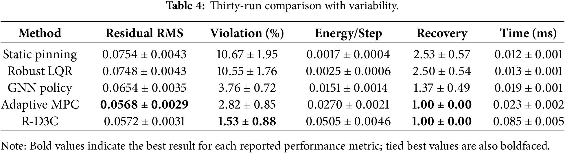
Fig. 4 shows the paired trajectories and their variability. The vertical markers indicate impulse disturbances. R-D3C suppresses the post-shock spread and returns to the low-risk region in one step on average, while static methods retain a broader tail.

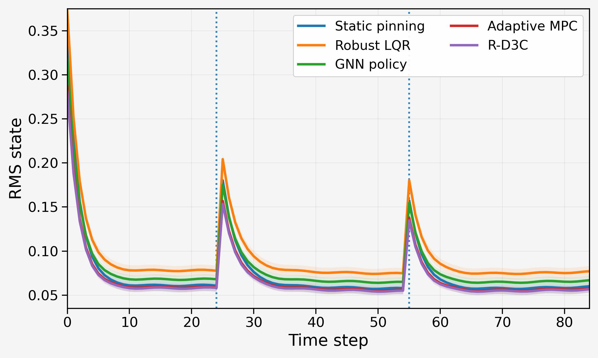
Figure 4: Mean RMS-state trajectories with one-standard-deviation bands over 30 runs.

Table 5 shows that the method is not hypersensitive to moderate changes in graph regularization, horizon, envelope coefficient, or decay margin. The intervention budget has the clearest effect: larger budgets reduce residual and violations but increase energy. We therefore use ℬ=8 as a balanced operating point.

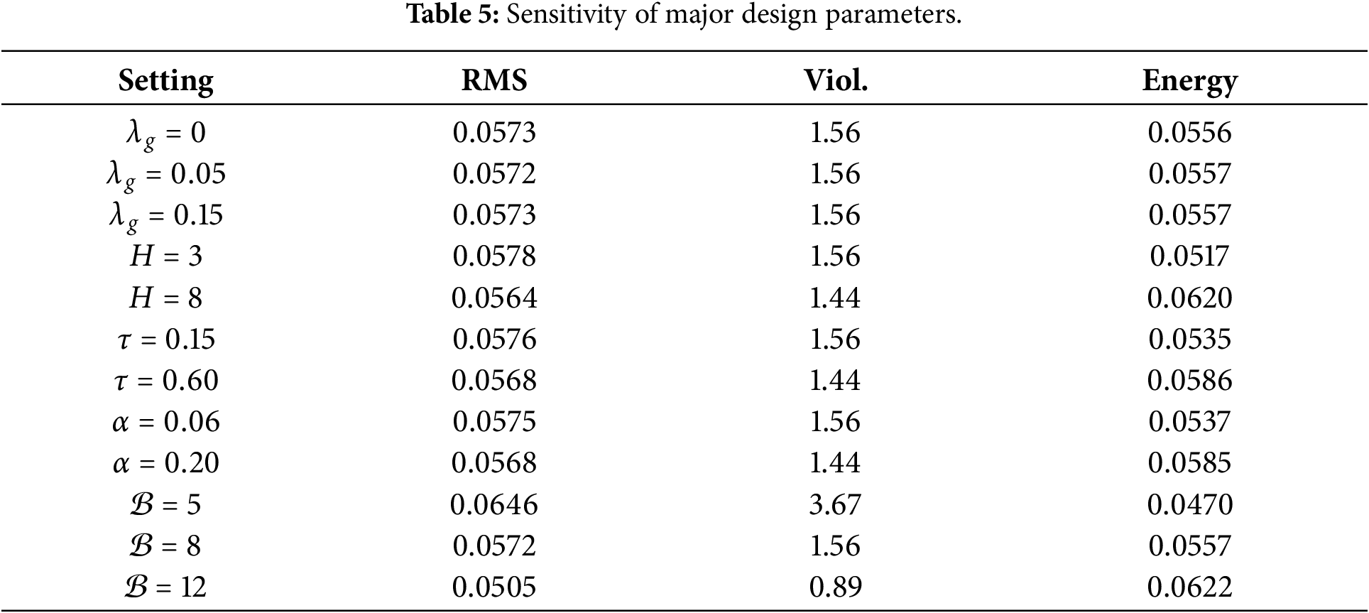
Fig. 5 visualizes the measured stabilization boundary over intervention budget and disturbance multiplier.

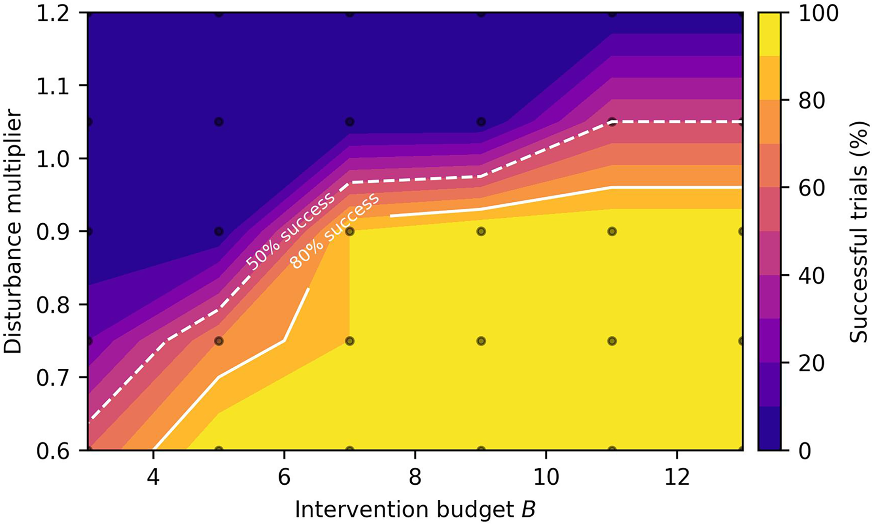
Figure 5: Measured stabilization boundary over budget and disturbance multiplier.

Table 6 uses 20 independent random seeds for every listed topology/impairment row. Communication delay has the highest constraint-violation rate (4.41%) and the slowest recovery (2.15 steps), whereas sensor-noise increase produces the largest residual RMS (0.0700 vs. 0.0616 for delay). We therefore do not rank delay as universally “hardest.” When a single impairment-severity criterion is needed, we prioritize violation rate because it directly counts breaches of the prescribed safety constraint, while residual RMS is a tracking-performance metric; recovery time is used as a secondary safety-resilience indicator. Radius inflation and the fallback keep the tested residuals bounded, but delay-dependent certificates remain future work.

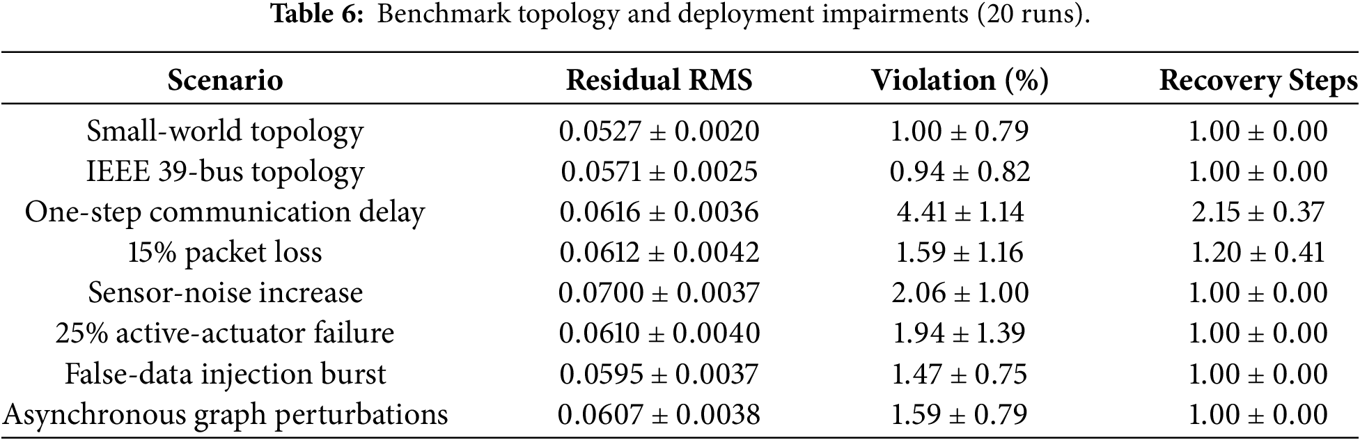
Table 7 is a computation-time microbenchmark only and intentionally reports no residual-RMS or constraint-violation values for the 200–1000-node timing cases. It is therefore not used to claim closed-loop accuracy or safety at those scales. The timing data support real-time use at moderate scale and sub-100-ms execution at 1000 nodes on the reported CPU. The dominant cost is graph-regularized identification; node-local parallel blocks reduce memory from a dense global inverse and are required on edge devices. Communication consists of local state, residual, and certificate summaries, i.e., O(df+degi) values per active node per update. The timings in Table 7 were obtained with the scalable node-local implementation summarized in Table 3, rather than a dense global inverse. The node-local blocks are parallelizable across nodes, but the reported benchmark is the end-to-end wall-clock time of the stated Python/NumPy CPU implementation and is not an ideal-parallel timing model. It uses node-local identification blocks, cached low-rank Gramian updates, batched linear algebra, and warm-started MPC. The budget ℬ=8, horizon H=5, window length m=12, and local feature dimension were held fixed as n increased. Hence the nominal dimensions of the MPC and projection subproblems do not grow with n, whereas implementation-level block assembly, indexing, memory traffic, and batched-kernel overhead collectively increase with network size. Over the full range, n increases by 1000/60=16.7 while measured time increases by 36.0/0.097≈371; the corresponding descriptive endpoint exponent is log⁡(371)/log⁡(16.7)≈2.10. This finite-range exponent summarizes the measured implementation only and is not an estimate of the asymptotic algorithmic order. The observed end-to-end timing is superlinear and roughly quadratic over the tested range, while the uneven local ratios (about 6.1×, 13.6×, and 4.5×) show that a single empirical power law is not appropriate. Because no component-level profiler was used in this timing experiment, the exponent is not attributed to any single kernel or module. Table 3 therefore gives module-level operation counts and parallelizable structure rather than a prediction of the wall-clock exponent of this Python implementation.

Fig. 6 summarizes the normalized residual, violation, energy, and recovery costs across the compared methods.

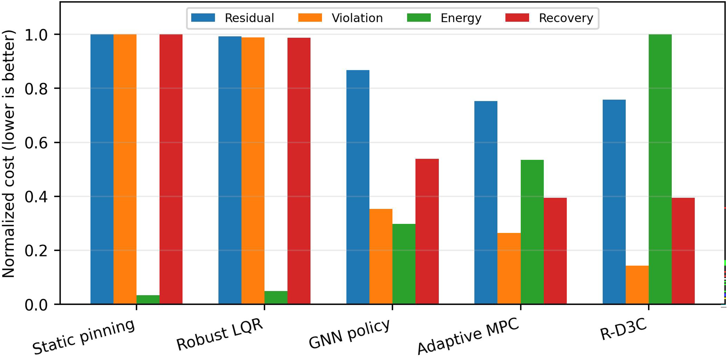
Figure 6: Normalized residual, violation, energy, and recovery costs.

6.2 Discussion

The experiments support four conclusions. First, adaptive MPC can match the residual accuracy of R-D3C, but the robust projection materially reduces constraint violations. Second, the safety advantage has a measurable energy and runtime cost, which should be considered when tuning α, H, and ℬ. Third, the IEEE 39-bus test indicates that the allocation mechanism transfers beyond random graphs, although it is not a substitute for field-event validation. Fourth, one-step communication delay causes the highest violation rate and slowest recovery, whereas increased sensor noise causes the largest residual RMS; this metric-dependent distinction motivates both delay-aware safety certificates and improved noise-robust prediction. The 1000-node result in Table 7 supports computational timing only; it does not extend the safety or violation-rate claims beyond the closed-loop experiments for which those quantities were explicitly measured.

Implementation on an edge platform requires a bounded local feature dimension, warm starts, cached Gramian updates, and event-triggered exchange of only residual and certificate summaries. Strict safety is claimed only when the projection has zero slack. When slack is positive, the controller records the event, expands the active set, and applies the backup action; operators can therefore distinguish certified from best-effort intervals.

7  Conclusion and Future Work

This paper developed R-D3C for disturbed complex networks with changing dynamics and a limited actuator budget. The framework combines the implemented sliding-window graph estimator, disturbance-envelope adaptation, sparse allocation, receding-horizon control, and robust projection. The analysis provides practical stability on certified zero-slack intervals, a sparse risk-reduction guarantee, and dynamic regret for the implemented windowed estimator. A checkable feasibility condition and explicit slack-and-backup rule clarify what happens when strict projection is unavailable. The evaluation separates a 30-run nominal comparison from the 20-run deployment-impairment benchmark, and also includes the IEEE 39-bus topology and 1000-node timing. The 1000-node result is interpreted strictly as a computation-time microbenchmark rather than a safety validation. R-D3C attains the lowest violation rate, while adaptive MPC remains statistically tied in residual accuracy.

Future work will focus on three issues: delay-dependent robust invariance for stale and asynchronous measurements; field-data calibration on power, traffic, and industrial logs rather than topology-only benchmarks; and fully distributed certificates with event-triggered communication and hardware-in-the-loop validation.

Acknowledgement: Not applicable.

Funding Statement: The authors received no specific funding for this study.

Availability of Data and Materials: The data that support the findings of this study are available from the corresponding authors upon reasonable request.

Author Contributions: The authors confirm contribution to the paper as follows: Conceptualization, Xiusen Wang; methodology, Xiusen Wang; software, Xiusen Wang; formal analysis, Xiusen Wang; visualization, Xiusen Wang; writing—original draft preparation, Xiusen Wang; validation, Jie Chen; supervision, Jie Chen; project administration, Jie Chen; writing—review and editing, Zheng Fang and Jie Chen. All authors reviewed and approved the final version of the manuscript.

Ethics Approval: Not applicable. This study did not involve human participants or animals.

Conflicts of Interest: Given his role as an Editorial Board Member/Guest Editor of this journal, Jie Chen had no involvement in the peer review of this article and had no access to information regarding its peer review. Full responsibility for the editorial process for this article was delegated to another journal editor. The authors declare no conflicts of interest.

References

1. Watts DJ, Strogatz SH. Collective dynamics of ‘small-world’ networks. Nature. 1998;393(6684):440–2. doi:10.1515/9781400841356.301. [Google Scholar] [CrossRef]

2. Baggio G, Bassett DS, Pasqualetti F. Data-driven control of complex networks. Nat Commun. 2021;12(3):1429. doi:10.1093/nsr/nwu024. [Google Scholar] [CrossRef]

3. Jia J, van Waarde HJ, Trentelman HL, Camlibel MK. A unifying framework for strong structural controllability. IEEE Trans Automat Contr. 2021;66(1):391–8. doi:10.1109/tac.2020.2981425. [Google Scholar] [CrossRef]

4. van Waarde HJ, Camlibel MK, Mesbahi M. From noisy data to feedback controllers: nonconservative design via a matrix S-lemma. IEEE Trans Automat Contr. 2022;67(1):162–75. [Google Scholar]

5. Ali M, Duchesne F, Dahman G, Gagnon F, Naboulsi D. New approaches for network topology optimization using deep reinforcement learning and graph neural network. IEEE Access. 2025;13:85447–60. doi:10.1109/access.2025.3569236. [Google Scholar] [CrossRef]

6. Kashima K, Yoshiuchi R, Wang R, Kawano Y. A unified framework for dynamics modeling and control design using deep learning with side information on stabilizability. IEEE Trans Neural Netw Learn Syst. 2025;36(8):15244–54. doi:10.1109/tnnls.2025.3543926. [Google Scholar] [CrossRef]

7. Pasqualetti F, Zampieri S, Bullo F. Controllability metrics, limitations and algorithms for complex networks. IEEE Trans Control Netw Syst. 2014;1(1):40–52. doi:10.1109/tcns.2014.2310254. [Google Scholar] [CrossRef]

8. Summers TH, Cortesi FL, Lygeros J. On submodularity and controllability in complex dynamical networks. IEEE Trans Control Netw Syst. 2016;3(1):91–101. doi:10.1109/tcns.2015.2453711. [Google Scholar] [CrossRef]

9. Olshevsky A. Minimal controllability problems. IEEE Trans Control Netw Syst. 2014;1(3):249–58. doi:10.1109/tcns.2014.2337974. [Google Scholar] [CrossRef]

10. Pequito S, Kar S, Aguiar AP. A framework for structural input/output and control configuration selection in large-scale systems. IEEE Trans Automat Contr. 2016;61(2):303–18. doi:10.1109/tac.2015.2437525. [Google Scholar] [CrossRef]

11. Cao K, Hu S, Shi Y, Colombo AW, Karnouskos S, Li X. A survey on edge and edge-cloud computing assisted cyber-physical systems. IEEE Trans Ind Inform. 2021;17(11):7806–19. doi:10.1109/tii.2021.3073066. [Google Scholar] [CrossRef]

12. Dong S, Tang J, Abbas K, Hou R, Kamruzzaman J, Rutkowski L, et al. Task offloading strategies for mobile edge computing: a survey. Comput Netw. 2024;254(6):110791. doi:10.1016/j.comnet.2024.110791. [Google Scholar] [CrossRef]

13. Zhang S, Yi N, Ma Y. A survey of computation offloading with task types. IEEE Trans Intell Transp Syst. 2024;25(8):8313–33. doi:10.1109/tits.2024.3410896. [Google Scholar] [CrossRef]

14. Wu J, Xu X, Cui G, Jiang J. Joint optimization of computation offloading and resource allocation in heterogeneous UAV-assisted edge computing: a game-theoretical approach. IEEE Trans Netw Sci Eng. 2026;13:8348–61. doi:10.1109/tnse.2026.3680337. [Google Scholar] [CrossRef]

15. Chen Z, Yang Y, Xu J, Chen Y, Huang J. Task offloading and resource pricing based on game theory in UAV-assisted edge computing. IEEE Trans Serv Comput. 2025;18(1):440–52. doi:10.1109/tsc.2024.3512936. [Google Scholar] [CrossRef]

16. Darchini-Tabrizi M, Roudgar A, Entezari-Maleki R, Sousa L. Distributed deep reinforcement learning for independent task offloading in mobile edge computing. J Netw Comput Appl. 2025;240(6):104211. doi:10.1016/j.jnca.2025.104211. [Google Scholar] [CrossRef]

17. Raju LR, Reddy MVK, Surukanti SR, Sudhakar G, Subrahmanya Sarma MVV, Adepu A. IntelliScheduler: an edge-cloud computing environment hybrid deep learning framework for task scheduling based on learning. Sci Rep. 2026;16(1):11219. doi:10.1038/s41598-026-41330-8. [Google Scholar] [CrossRef]

18. Farooq A, Xiang Z, Chang W-J, Aslam MS. Recent advancement in formation control of multi-agent systems: a review. Comput Mater Contin. 2025;83(3):3623–74. doi:10.32604/cmc.2025.063665. [Google Scholar] [CrossRef]

19. Alasbali N. Deep multi-agent stochastic optimization for traffic management in IoT-enabled transportation networks. Comput Mater Contin. 2025;85(3):4943–58. doi:10.32604/cmc.2025.068330. [Google Scholar] [CrossRef]

20. D’Souza RM, di Bernardo M, Liu Y-Y. Controlling complex networks with complex nodes. Nat Rev Phys. 2023;5(4):250–62. doi:10.1038/s42254-023-00566-3. [Google Scholar] [CrossRef]

21. Wu H, Lu Y, Ma H, Xing L, Deng K, Lu X. A survey on task type-based computation offloading in mobile edge networks. Ad Hoc Netw. 2025;169(2):103754. doi:10.1016/j.adhoc.2025.103754. [Google Scholar] [CrossRef]

22. Dai Y, Li M, Zhang K, Shi Y. Robust and resilient distributed MPC for cyber-physical systems against DoS attacks. IEEE Trans Ind Cyber Phys Syst. 2023;1(1):44–55. doi:10.1109/ticps.2023.3283229. [Google Scholar] [CrossRef]

23. Xu K, Sadaf F, Niazi AUK, Samman FMA, Almazah MMA, Smerat A. Resilient fuzzy adaptive control of fractional-order multi-agent systems under input constraints and cyber attacks. Iran J Sci Technol Trans Electr Eng. 2026;8(9):8045803. doi:10.1007/s40998-026-01060-z. [Google Scholar] [CrossRef]

24. Zimmerman RD, Murillo-Sánchez CE, Thomas RJ. MATPOWER: steady-state operations, planning, and analysis tools for power systems research and education. IEEE Trans Power Syst. 2011;26(1):12–9. [Google Scholar]