High-Precision Time Delay Estimation Based on Closed-Form Offset Compensation

1  Introduction

The time delay estimation (TDE) is a key issue of the time difference of arrival (TDOA) method [1–3], which plays a crucial role in passive localization positioning, navigation, wireless communication, electronic countermeasures and wireless sensor networks, etc. [4–11]. In the field of positioning, TDOA-based method locates the source by estimating the time difference among different nodes arriving at the target, which avoids the requirement for node sensor clocks to be synchronized with the target in the TOA method [12–14]. Obviously, the TDE directly affects the performance of positioning. Hence, it is of great concern to study high accurate TDE methods.

Generalized cross correlation (GCC) [15–17] is a classical approach for TDE, it applies a weighting function to the cross-power spectrum to improve the signal-to-noise ratio (SNR) and thus sharpen the peak of the correlation function. In various GCC methods, the GCC with phase transform (GCC-PHAT) method can make the TDE robust against noise and reverberation and thus has better performance than others [18–20]. On the strength of the GCC, some new methods have been proposed for high-precision TDE. A closed-form maximum-likelihood cross-phase spectrum estimation method for GCC is proposed in [21], which corrects the phase bias by noise coherence function to obtain accurate TDE. The paper in [22] extracts GCCs based on the sliding-window method and uses sub-band GCC to represent the corresponding cross-power spectrum phase, but the temporal resolution is reduced. Based on GCC-PHAT, the ‘inversed’ diffuseness is binarized with a strict threshold, which masks the time-frequency components of observed signals to obtain reliable TDE [23]. However, these methods fail to address the problem of the limited resolution, and the fact that the calculated TDE is always integer multiple of the sampling period. A self-delay-compensation (SDC) method is proposed to solve this problem in [24]. By adding a tiny time delay unit, this method makes up the neglectful time delay within a sampling interval. In addition, some super-resolution TDE methods are proposed to overcome the limited sampling period. Utilizing sinusoidal signal frequency estimation model, Ge et al. [25] constructs covariance matrix through signal correlation, and adopts multiple signal classification (MUSIC) algorithm for TDE. But it needs to estimate the power spectrum density of the unknown signal at first. A super-resolution method using normalized cross spectrum is proposed to estimate time delay in [26], which makes the feature structure of signal normalized cross spectrum to deduce a new TDE model. Compared with [25], it avoids estimating the power spectrum of unknown signals and reduces the amount of computation. Nevertheless, the above methods belong to subspace-based algorithms, and they inevitably suffer from high computational complexity due to eigenvalue decomposition (EVD) and spectral peak search.

In this paper, we propose an efficient TDE method for TDOA-based passive localization, which overcomes the problem of limited sampling intervals. The contributions of our work are summarized as follows:

(1)   Based on the first-order Taylor expansion on the vector containing initial TDEs, high accurate time delays are estimated by adding closed-form offset compensation obtained via least squares (LS).

(2)   Theoretical analysis and simulation experiments are conducted, which demonstrate that the proposed method has lower computational complexity and more accurate estimation compared with SDC [24] and MUSIC [26] methods.

(3)   Experiments on real-world scenarios demonstrate that the proposed method significantly improves the performance of source localization.

Notation: Vectors are represented by lowercase bold characters and matrices by uppercase bold characters. (⋅)T and (⋅)H represent transpose and conjugate-transpose, respectively. ∂(a)/∂(b) means the derivative of a with respect to b. E(⋅) denotes expectation. |⋅| represents the modulus of a complex number. ⌊⋅⌋ and ⌈⋅⌉ stand for the floor and ceiling function, respectively. arg⁡max(⋅) represents arguments of the maxima. diag(⋅) denotes the diagonal matrix. x^ represents the estimated version of x. (⋅)+ denotes the pseudo inverse of a matrix.

2  Signal Model

To better explain the TDOA localization principle, Fig. 1 presents a passive positioning system with multi-nodes. There are M(M≥3) nodes randomly distributed in qi=[xi,yi]T,i=1,…,M. The radiation source emits signal, which is then picked up by the sensors on nodes. And clock synchronization of multiple nodes is implemented as to collect TDOA measurements. The target source location is u=[x,y]T.

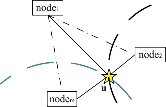
Figure 1: TDOA positioning system based on multi-nodes

Suppose that s(t) is the signal emitted by the target source in line-of-sight case. Then the signal received by the m-th node can be expressed as

xm(t)=αms(t−τm)+nm(t),m=1,2,…,M(1)

where αm is amplitude fading coefficient, τm is time delay between the target source and the m-th node, and nm(t) denotes the zero-mean additive Gaussian noise of the m-th received signal. By estimating the time differences among the source signal reaching the reference node and other nodes, the distance differences of them can be calculated. Next, a set of hyperbolic equations is established to depict these hyperboloids whose intersection is the desired target position as shown in Fig. 1.

3  Proposed Scheme

Just like the system model introduced above, a passive positioning system is composed of M(M≥3) nodes. The signals received by nodes are as follows:

{x1(t)=α1s(t−τ1)+n1(t)x2(t)=α2s(t−τ2)+n2(t)⋮xM(t)=αMs(t−τM)+nM(t)(2)

3.1 The Initial TDE Based on GCC

Generally, the received signal at first node x1(t) is selected as the reference signal. Due to only the time difference of arrival is needed in the passive positioning system based on TDOA, we can assume α1=1 and τ1=0 for simplified analysis. From Eq. (2) we can get

{x1(t)=s(t)+n1(t)xm(t)=αms(t−τ1,m)+nm(t)m=2,3,…,M(3)

where τ1,m=τm−τ1 represents the time difference among the source signal reaching the reference node and other nodes. The cross-correlation function of the two signals from Eq. (3) is

Rx1xm(τ)=E[x1(t)xm(t−τ)]=αmE[s(t)s(t−τ1,m−τ)]+E[s(t)nm(t−τ)]+αmE[s(t−τ1,m−τ)n1(t)]+E[n1(t)nm(t−τ)](4)

Assuming that s(t) and nm(t)(m=1,2,…,M) are independent, Eq. (4) can be simplified as

Rx1xm(τ)=αmE[s(t)s(t−τ1,m−τ)]=αmRss(τ−τ1,m)(5)

According to Wiener-Khinchin theorem, the discrete Fourier transform (DFT) of the correlation function is the corresponding power spectrum. In the GCC method, the received signal is weighted in frequency domain to enhance the frequency component with high SNR and suppress the noise power. Here the PHAT is chosen due to its robustness, whose weighting function is φ1m(ω)=1/|Gx1xm(ω)|. The GCC function is expressed as the inverse Fourier transform of the weighted power spectral function φ1m(ω)Gx1xm(ω).

Rx1xmg(τ)=12π∫−∞∞1|Gx1xm(ω)|Gx1xm(ω)ejωτdω(6)

where Gx1xm(ω) is the cross-power spectrum of the received signals. By looking for the abscissa parameter corresponding to the maximum of GCC-PHAT, the TDEs can be calculated via

τ^1,mini=arg⁡maxτ⁡Rx1xmg(τ),m=2,3,…,M(7)

Therefore, the initial TDEs are obtained by Eq. (7). However, the resolution of this method is limited by sampling period. In fact, we can estimate time delay by the subspace method which can break through the restriction of sampling period. The super-resolution method using normalized cross spectrum in [26] derives the orthogonal formula containing initial delay, and no relevant transcendental knowledge is needed.

3.2 Normalized Cross Spectrum

Using the signal model shown in Eq. (3) above, on the assumption that the signal is not correlated with the noise, the autocorrelation function of the reference signal x1(t) is

Rx1x1(τ)=E[x1(t)x1(t−τ)]=Rss(τ)+Vn1n1(τ)(8)

where Rss(τ) and Vn1n1(τ) are the autocorrelation functions of s(t) and n1(t), respectively. According to Wiener-Khinchin theorem, the power spectrum of x1(t) can be obtained by

Gx1x1(ω)=Gss(ω)+Nn1n1(ω)(9)

where Gss(ω) and Nn1n1(ω) are the Fourier transform of Rss(τ) and Vn1n1(τ), respectively. The cross-power spectrum of x1(t) and xm(t) can be formulated from Eq. (5).

Gx1xm(ω)=αmGss(ω)e−jωτ1,m(10)

The cross-power spectrum of the two observed signals has the following relationship with the power spectrum of x1(t) as

Gx1xm(ω)=αm(Gx1x1(ω)−Nn1n1(ω))e−jωτ1,m(11)

Using Gx1x1(ω) to normalize cross-power spectrum Gx1xm(ω) as follows:

h(ω)=αme−jωτ1,m+u(ω)(12)

where h(ω)=Gx1xm(ω)/Gx1x1(ω) is normalized cross power spectrum, u(ω)=−(Nn1n1(ω)/Gx1x1(ω))αme−jωτ1,m. The noise u(ω) obeys the Gaussian distribution. In order to suppress the effect of noise u(ω) in the model, we select the effective part of the uniform extraction of h(ω) in the frequency domain to define the observation vector

hd=αm⋅ad(τ1,m)+ud(13)

where

hd=[h(ωb+d−1),h(ωb+d−1+D),⋯,h(ωb+d−1+(P−1)D)]T,d=1,2,⋯,D,

ad(τ1,m)=[e−j(ωb+d−1)τ1,m,e−j(ωb+d−1+D)τ1,m,…,e−j(ωb+d−1+(P−1)D)τ1,m]T,

ud=[u(ωb+d−1),u(ωb+d−1+D),…,u(ωb+d−1+(P−1)D)]T.

where ωb is the lower bound angle frequency of the cross-power spectrum bandwidth of the two signals, which can be obtained by calculating the Gx1xm(ω) and setting the threshold for detection. D is the uniform extraction interval that constitutes the observation vector, and P is the length of the observation vector, which needs to be met P>D and ωb+PD−1<2L−1. Then the normalized cross-power spectrum vector model can be written as

H=αm⋅A+V(14)

where

H=[h1,h2,⋯,hD]

A=[a1(τ1,m),a2(τ1,m)⋯,aD(τ1,m)]

V=[u1,u2,⋯,uD].

It can be seen that the normalized cross-power spectrum model is equivalent to the parametric model of line spectra. Therefore, the method of super-resolution spectrum estimation can be applied to estimate the time delay, such as MUSIC algorithm. The covariance matrix of H is

R=E[HHH](15)

It can be divided into signal subspace US and noise subspace UN by performing the EVD of covariance matrix R like

R=USΣSUSH+UNΣNUNH(16)

where, ΣS and ΣN represent the diagonal matrix composed of corresponding eigenvalues. Similar to the derivation of MUSIC algorithm, ad(τ1,m) is orthogonal to UN, i.e.,

adH(τ1,m)UN=0(17)

According to the orthogonal relation, the spectral function of time delay estimation is obtained

Pmusic(τ1,m)=1adH(τ1,m)UNUNHad(τ1,m)(18)

Then τ^1,m,m=2,3,…,M can be derived from the maxima of Pmusic(τ1,m) by one-dimensional search on τ1,m.

As a matter of fact, the subspace-based TDE methods need a wide time frame search, while direction of arrival (DOA) estimation only requires an angle search of −180 to 180. Moreover, the search interval of MUSIC method in [26] is less than 1/fs to get better estimates than GCC method, where fs is the sampling frequency. Besides, the fact that the calculated TDE using GCC is always integer multiple of the sampling period. It is not guaranteed that the actual time delay will fall exactly at the sampling point. In short, the theoretical best estimation is either ⌊τ1,m⋅fs⌋ or ⌈τ1,m⋅fs⌉, which always has estimated biases. The SDC algorithm in [24] searches for a tiny time delay compensation for more accurate estimation. Whereas, these approaches require multiple searches within a time orderly to get the optimal compensation, which greatly increases the calculated amount. Unlike them, the GCC-PHAT method estimating time differences is considered that are close to the real ones. Hence, the first-order Taylor expansion is performed on the initial TDEs to get the closed-form offset compensation.

3.3 Closed-Form Offset Compensation

Since the GCC method cannot overcome the limitation that the resolution is the sampling period, the time delay τ^1,mini obtained in the Section 3.1 is off the exact value, so we need to compensate it. The orthogonal relation between noise characteristic vector UN and delay vector ad(τ1,m) obtained in Section 3.2 can be obtained as follows:

UNHad(τ1,m)=0(19)

Next, we apply the first order Taylor expansion to ad(τ1,m) so we can get

ad(τ1,m)≈atd(τ^1,mini)+∂ad(τ^1,mini)∂τ^1,mini⋅ξm(20)

where τ^1,mini is initial TDE from Eq. (7), and ξm=τ1,m−τ^1,mini, then Eq. (19) is rewritten as

UNH(ad(τ^1,mini)+∂ad(τ^1,mini)∂τ^1,mini⋅ξm)=0(21)

The offset ξm that is the difference between true time delay and initial estimated time delay can be calculated via LS.

ξ^m=−(UNH∂ad(τ^1,mini)∂τ^1,mini)+UNHad(τ^1,mini)(22)

By compensating offset ξ^m, high precision delay estimation can be calculated as

τ^1,m=τ^1,mini+ξ^m,m=2,3,⋯,M(23)

In most cases, iterations are necessary during Taylor expansion method implementation. Fig. 2 depicts the iterative process of the proposed method in detail. The number of iterations is indicated by i, whose value is determined by the residual. For example, if the compensation value approaches zero, the iteration should be stopped at this time. After iteration, high-precision TDE can be obtained. Furthermore, the complexity of this method after iteration is also low, as will be discussed in detail below.

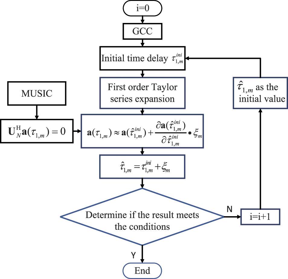
Figure 2: Flow chart of the proposed method with iterations

Then we list the corresponding hyperbolic equations after acquiring more accurate TDEs based on Eq. (23) via

c⋅τ^1,m=(x−xm)2+(y−ym)2+(z−zm)2−(x−x1)2+(y−y1)2+(z−z1)2(24)

where c is the wave propagation speed. It is well known that the Chan algorithm [27] tends to be affected by the accuracy of TDEs, we can derive an optimal location estimation based on the improvement of TDEs.

3.4 Detailed Procedures

Generally, the method in this paper mainly includes the following steps:

1)   Select the received signal x1(t) as reference signal, then use the GCC-PHAT method to calculate initial TDE τ^1,mini by Eq. (7).

2)   The TDE model is derived from the normalized cross-power spectrum of observed signals as Eq. (14), and the corresponding noise subspace UN is obtained by eigenvalue decomposition of covariance matrix from Eq. (16).

3)   According to the orthogonal relation of UN and ad(τ1,m) which contains initial TDE, just like Eq. (19), the first-order Taylor expansion is performed on ad(τ1,m) in Eq. (20), then figure up the closed-form offset compensation ξ^m by Eq. (22) on the basis of LS.

4)   Calculate the fine time delay estimations τ^1,m via Eq. (23), then establish corresponding hyperbolic equations, and finally derive the source position estimation through the Chan algorithm.

4  Performance Analysis

4.1 Complexity Comparison

This section is presented to discuss the computational complexity of different methods. The computation cost of GCC-PHAT is about O((2M−1)Llog2L+(M−1)L)), where L is the number of sampling points. The computation of SDC is record as O(Llog2L+J(M−1)(2Llog2L+3L)), where J denotes the number of searches within a sampling interval. For the MUSIC, the complexity is O((2M−1)(Llog2L+L)+(M−1)(P3+D2P)+Q(M−1)P(2P−1)), where P denotes number of spectral peak searches. The computational complexity of the proposed method is O((2M−1)Llog2L+ML+(M−1)(P3+D2P)+i(M−1)(2P2+P)), where i is the number of iterations. Specifically, calculating the initial TDE τ^1,mini requires O((2M−1)Llog2L+(M−1)L)) using GCC-PHAT method and adding closed-form offset compensation costs O(L+(M−1)(P3+D2P)+i(M−1)(2P2+P)). The computational complexity of compensation depends on EVD in Eq. (16) and LS in Eq. (22).

Fig. 3 demonstrates computational complexities comparison among the GCC-PHAT, SDC, MUSIC, and proposed method under the condition that L=2048, J=10, Q=200, D=50, P=50, i=2. Here we select different values of M to compare. It is observed that the complexity of the proposed method is greatly lower compared to the SDC and MUSIC methods. Even after iterations, the proposed method still has a low complexity, which commendably verifies the superiority of this method.

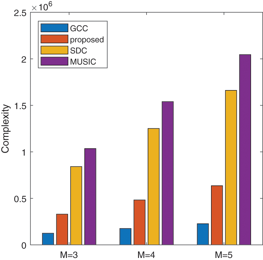
Figure 3: The comparison of complexity among different methods

4.2 Simulation Results

This part mainly presents simulation experiments to test the methods. Assuming that the nodes number is M=3, their positions in the cartesian coordinate are q1=(100,200), q2=(500,1000), q3=(1500,1500), separately. Position of the source is u=(35,170). All of these coordinates are in meter. Here the source transmits a LFM signal with time-width t=5×10−6 s and signal bandwidth B=30MHz. Let root mean square error (RMSE) measure the estimated performance of each method, the RMSE can be expressed as

RMSE=1K∑i=1K(τ^i−τ)2(25)

where K is Monte-Carlo simulation times, τ represents actual time delay and τ^i represents estimated time delay of the i-th Monte-Carlo experiment. For each simulation, 1000 Monte Carlo experiments are achieved.

Fig. 4 illustrates the RMSE performances of the TDE algorithms vs. SNR, including the GCC, MUSIC, SDC, and the proposed method. Experiments are conducted with the setting sampling frequency fs=125MHz, and sampling points L=2048. As can be seen from Fig. 4, the MUSIC method changes greatly with the increase of SNR, which is sensitive to SNR and sampling points. Although the SDC method is better than the GCC method, it still has the defect of unsearchable interval. The proposed method not only improves the performance of estimation accuracy, but also has the advantage of low complexity.

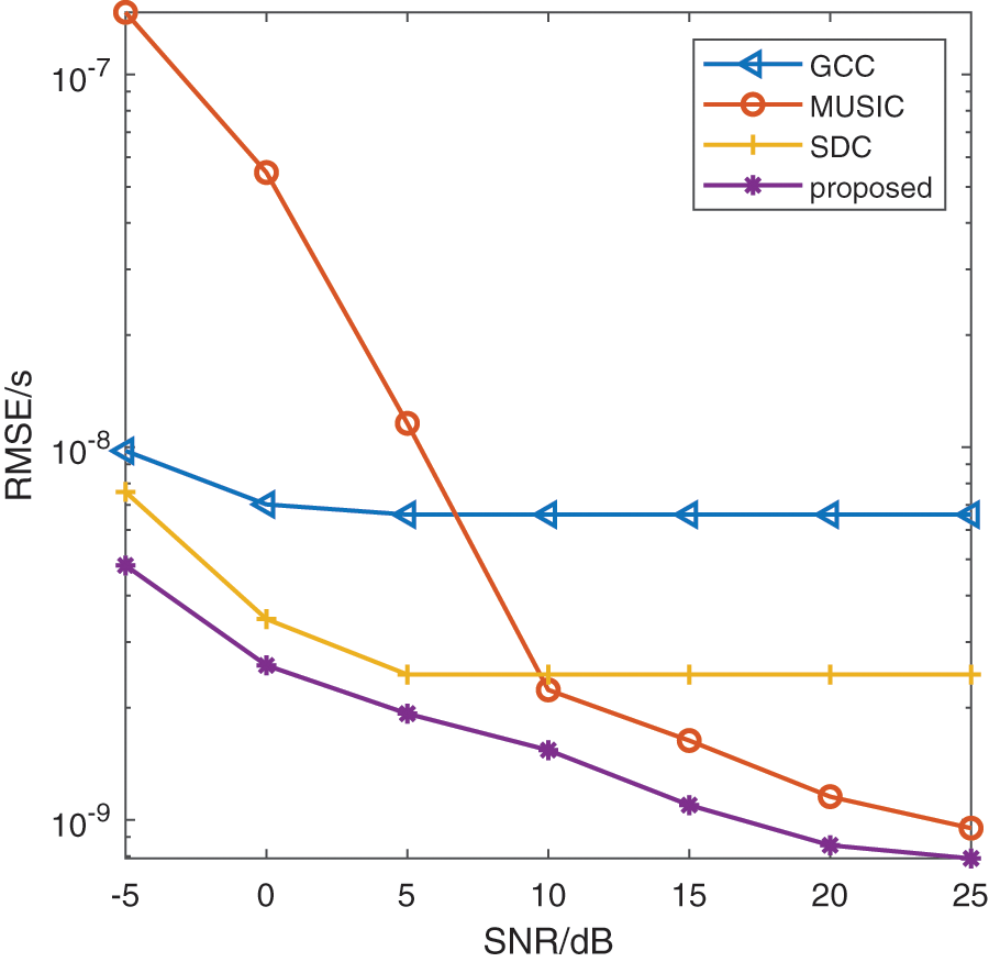
Figure 4: TDE performance comparison versus SNR

Meanwhile, the time delay estimation comparison of different methods between signal source arrival at q3, q2 and reference node q1 is shown in Fig. 5, where τq2q1=2.9326×10−6 s, τq3q1=6.3569×10−6 s. The horizontal axis in the figure represents the time delay. It shows the time delay values estimated by each method, among which the proposed method successfully obtains the best estimation results by using offset compensation.

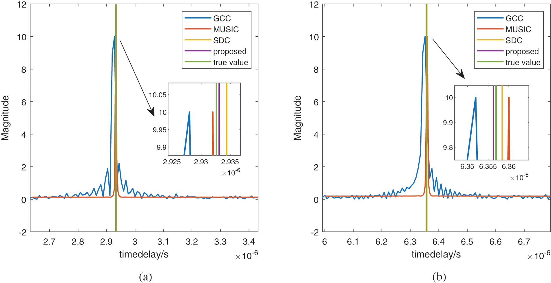
Figure 5: Time delay estimation comparison of different methods (a) Time delay τq2q1 (b) Time delay τq3q1

5  Real-World Testing

In this paper, the measured data collected in real-world experiments is used to further prove the validity of the proposed method. As shown in Fig. 6, there are three anchors in the campus namely anchor 1, anchor 2, and anchor 3, and the source is placed at the playground. In the experiment, the source transmits signals of various frequencies and modulation modes, which are received by the anchors. The computer remotely connects the three anchors to convert the collected data into the common Excel type for convenient data reading.

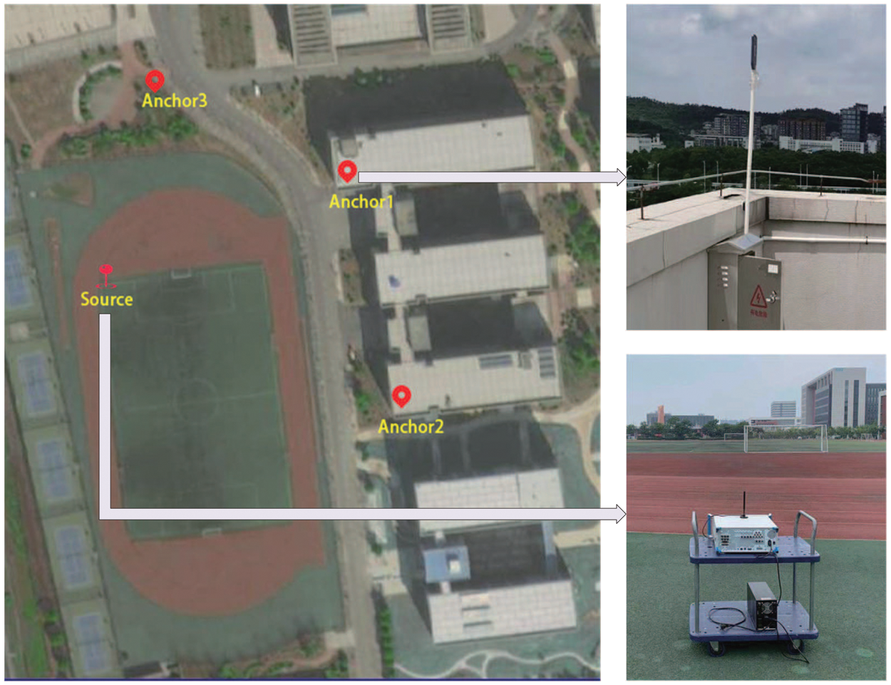
Figure 6: Actual test scenario of source and three anchors

To process the collected measured data, we choose anchor 3 as the reference anchor, and then estimate the time differences among the signal radiation reaching the anchor 3 and others. The radiation source is a wideband signal modulated by QPSK, the center frequency is 700 MHz with 30 MHz bandwidth, and the sampling frequency is fs=125MHz with L=32508 sampling points. Fig. 7 is a comparison of the actual time delay and the estimated time delay obtained by different methods. It is demonstrated in Fig. 7 that the time delay using the proposed approach is closer to the real value, which illustrates that the proposed approach is superior to other approaches.

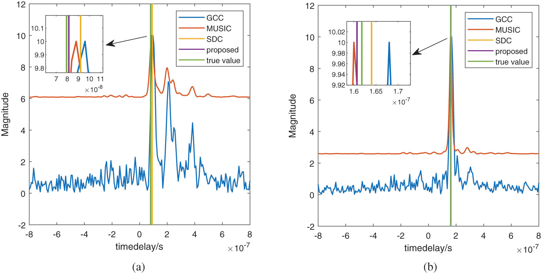
Figure 7: The TDEs based on measured data (a) Time delay τ1,3 (b) Time delay τ2,3

Fig. 8 is a coordinate chart of the positioning result. We choose anchor 3 as the reference origin to establish a two-dimensional coordinate system. The Chan algorithm [27] is used to locate the estimated signal source based on the time delay processed by the measured data. The red five-pointed star in the figure represents the actual source location, and the blue triangle represents the estimated source position based on the approach proposed in this paper. As is demonstrated from Fig. 8 that the two signs are very close to each other, indicating that the proposed method is practical.

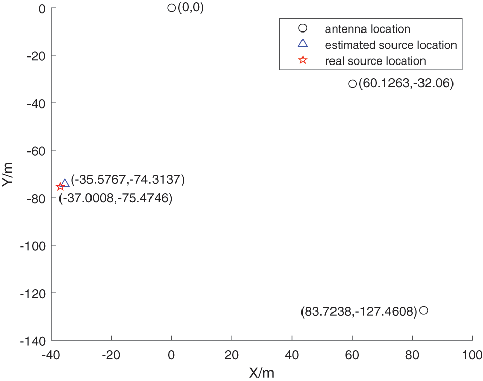
Figure 8: Actual test scenario of source and three anchors

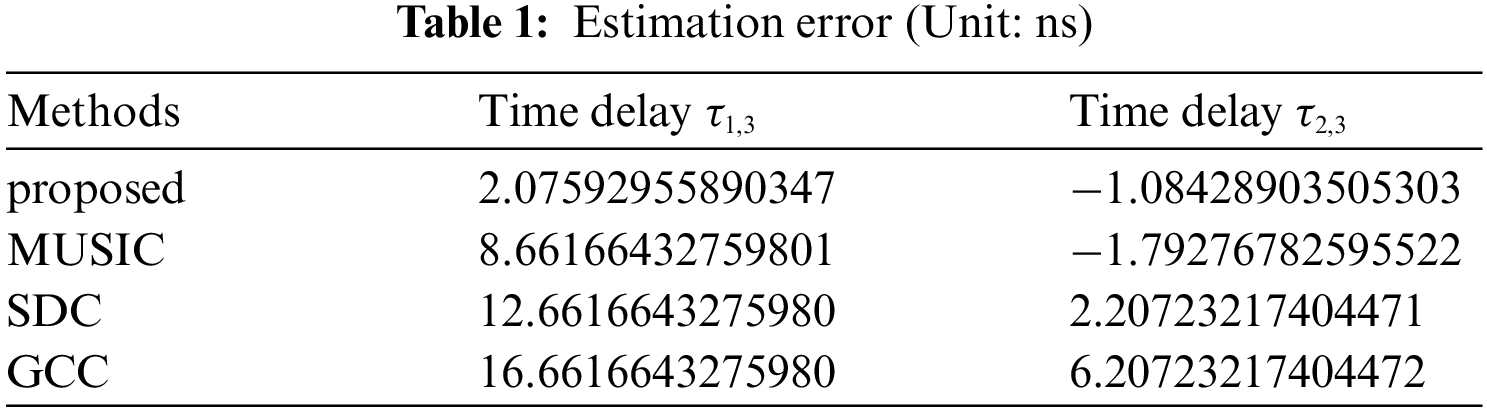
Table 1 shows the time delay estimation errors of the four methods among reference node and other nodes. It can be seen that the TDE performance of the method proposed in this paper is closer to the actual time delay compared with other methods.

6  Conclusion

This paper presents a high precision TDE method based on closed-form offset compensation. The initial TDEs are estimated by the GCC method. Then we make use of the orthogonality of the noise subspace and the delay vector to obtain equation. To compensate the error caused by limited resolution in GCC, the first-order Taylor expansion is considered. The improved estimations are achieved by adding closed-form offsets, which can be computed by simple LS. Simulation experiments show that our method offers more accurate TDE results as well as lower computational complexity. Finally, we make experiments under the real field condition, which demonstrates that our method provides high-precision TDE.

Acknowledgement: The authors would like to thank the editor of this article and the anonymous reviewer for their valuable suggestions and comments which greatly improved the presentation of this paper.

Funding Statement: This work was supported in part by National Key R&D Program of China under Grants 2020YFB1807602 and 2020YFB1807600, National Science Foundation of China (61971217, 61971218, 61631020, 61601167), the Fund of Sonar Technology Key Laboratory (Range estimation and location technology of passive target via multiple array combination), Jiangsu Planned Projects for Postdoctoral Research Funds (2020Z013), China Postdoctoral Science Foundation (2020M681585).

Conflicts of Interest: The authors declare that they have no conflicts of interest to report regarding the present study.

References

1. Delcourt, M., Le Boudec, J. Y. (2021). Tdoa source-localization technique robust to time-synchronization attacks. IEEE Transactions on Information Forensics and Security, 16, 4249–4264. DOI 10.1109/TIFS.2020.3001741. [Google Scholar] [CrossRef]
2. Chen, X., Wang, D., Yin, J., Wu, Y. (2018). Performance analysis and dimension-reduction taylor series algorithms for locating multiple disjoint sources based on tdoa under synchronization clock bias. IEEE Access, 6, 48489–48509. DOI 10.1109/ACCESS.2018.2860958. [Google Scholar] [CrossRef]
3. Zekavat, R., Buehrer, R. M. (2019). Source localization: Algorithms and analysis. In: Handbook of position location: Theory, practice, and advances, pp. 59–106. Wiley, New Jersey, USA. [Google Scholar]
4. Xiong, H., Chen, Z. Y., Yang, B. Y., Ni, R. P. (2015). Tdoa localization algorithm with compensation of clock offset for wireless sensor networks. China Communications, 12(10), 193–201. DOI 10.1109/CC.2015.7315070. [Google Scholar] [CrossRef]
5. Hemavathy, P. R., Shuaib, Y. M., Lakshmanaprabu, S. K. (2019). Design of smith predictor based fractional controller for higher order time delay process. Computer Modeling in Engineering & Sciences, 119(3), 481–498. DOI 10.32604/cmes.2019.04731. [Google Scholar] [CrossRef]
6. Wang, H., Li, X. W., Jhaveri, R. H., Gadekallu, T. R., Zhu, M. F. et al. (2021). Sparse bayesian learning based channel estimation in FBMC/OQAM industrial IoT networks. Computer Communications, 176, 40–45. DOI 10.1016/j.comcom.2021.05.020. [Google Scholar] [CrossRef]
7. Wen, F. Q., Shi, J. P., Zhang, Z. J. (2022). Generalized spatial smoothing in bistatic EMVS-MIMO radar. Signal Processing, 193, 108406. DOI 10.1016/j.sigpro.2021.108406. [Google Scholar] [CrossRef]
8. Wang, H., Xu, L. W., Yan, Z. Q., Gulliver, T. A. (2021). Low-complexity MIMO-FBMC sparse channel parameter estimation for industrial big data communications. IEEE Transactions on Industrial Informatics, 17(5), 3422–3430. DOI 10.1109/TII.9424. [Google Scholar] [CrossRef]
9. Chen, H., Ballal, T., Saeed, N., Alouini, M. S., Al-Naffouri, T. Y. (2020). A joint TDOA-PDOA localization approach using particle swarm optimization. IEEE Wireless Communications Letters, 9(8), 1240–1244. DOI 10.1109/LWC.5962382. [Google Scholar] [CrossRef]
10. Zhu, Y. T., Dong, C. X., Liu, S. Y., Dong, Y. Y., Zhao, G. Q. (2016). Passive localization using retransmitted TDOA measurements in the presence of sensor position errors. Acta Aeronautica et Astronautica Sinica, 37(2), 706–716. DOI 10.7527/S1000-6893.2015.0203. [Google Scholar] [CrossRef]
11. Hao, W., Cheng, C., Mo, D. E. A. (2020). Phase tracking approach for TDOA measurements in critical lunar spaceflights. Science China Information Sciences, 63(2), 235--237. DOI 10.1007/s11432-018-9812-x. [Google Scholar] [CrossRef]
12. Zhang, L., Zhang, T., Shin, H. S. (2021). An efficient constrained weighted least squares method with bias reduction for TDOA-based localization. IEEE Sensors Journal, 21(8), 10122–10131. [Google Scholar]
13. Li, X., Zhang, X. Y., Yu, X., Hu, Y. P. (2013). Modified cramer-rao bound for relative location estimation. Journal of Data Acquisition & Processing, 28(2), 195–200. DOI 10.3969/j.issn.1004-9037.2013.02.013. [Google Scholar] [CrossRef]
14. Deng, Z. L., Wang, H. H., Zheng, X. Y., Fu, X., Yin, L. (2019). A closed-form localization algorithm and GDOP analysis for multiple TDOAs and single TOA based hybrid positioning. Applied Sciences, 9(22), 4935. DOI 10.3390/app9224935. [Google Scholar] [CrossRef]
15. Knapp, C., Carter, G. (1976). The generalized correlation method for estimation of time delay. IEEE Transactions on Acoustics, Speech, and Signal Processing, 24(4), 320–327. DOI 10.1109/TASSP.1976.1162830. [Google Scholar] [CrossRef]
16. Wang, J., Yang, J. S. (2008). The research of time delay estimation method of general cross correlation with frequency difference. Signal Processing, 24(1), 112–114. DOI 10.3969/j.issn.1003-0530.2008.01.026. [Google Scholar] [CrossRef]
17. Ding, C., Chen, Z., Zhang, Z. T., Cheng, Y. S. (2021). Time delay estimation using cross-power spectrum phase. Journal of Electronics & Information Technology, 43(3), 803–808. DOI 10.11999/JEIT200584. [Google Scholar] [CrossRef]
18. Kim, U. H., Nakadai, K., Okuno, H. G. (2015). Improved sound source localization in horizontal plane for binaural robot audition. Applied Intelligence, 42(1), 63–74. DOI 10.1007/s10489-014-0544-y. [Google Scholar] [CrossRef]
19. Villadangos, J. M., Urena, J., Garcia-Dominguez, J. J., Jimenez-Martin, A., Hernandez, A. et al. (2021). Dynamic adjustment of weighted GCC-PHAT for position estimation in an ultrasonic local positioning system. Sensors, 21(21), 7051. DOI 10.3390/s21217051. [Google Scholar] [CrossRef]
20. Padois, T., Doutres, O., Sgard, F. (2019). On the use of modified phase transform weighting functions for acoustic imaging with the generalized cross correlation. Journal of the Acoustical Society of America, 145(3), 1546–1555. DOI 10.1121/1.5094419. [Google Scholar] [CrossRef]
21. Li, X. L. (2021). On correcting the phase bias of GCC in spatially correlated noise fields. Signal Processing, 180, 107859. DOI 10.1016/j.sigpro.2020.107859. [Google Scholar] [CrossRef]
22. Cobos, M., Antonacci, F., Comanducci, L., Sarti, A. (2020). Frequency-sliding generalized cross-correlation: A sub-band time delay estimation approach. IEEE/ACM Transactions on Audio, Speech, and Language Processing, 28, 1270–1281. DOI 10.1109/TASLP.6570655. [Google Scholar] [CrossRef]
23. Lee, R., Kang, M., Kim, B., Park, K., Lee, S. Q. et al. (2020). Sound source localization based on GCC-PHAT with diffuseness mask in noisy and reverberant environments. IEEE Access, 8, 7373–7382. [Google Scholar]
24. He, Y., Li, J., Zhang, X. (2020). Adaptive cascaded high-resolution source localization based on collaboration of multi-UAVs. China Communications, 17(4), 165–179. [Google Scholar]
25. Ge, F. X., Shen, D., Peng, Y., Li, V. O. K. (2007). Super-resolution time delay estimation in multipath environments. IEEE Transactions on Circuits and Systems I: Regular Papers, 54(9), 1977–1986. DOI 10.1109/TCSI.2007.904693. [Google Scholar] [CrossRef]
26. Zhong, S., Xia, W., Song, J., He, Z. (2013). Super-resolution time delay estimation in multipath environments using normalized cross spectrum. 2013 International Conference on Communications, Circuits and Systems (ICCCAS), pp. 288–291. Chengdu, China. DOI 10.1109/ICCCAS.2013.6765235. [Google Scholar] [CrossRef]
27. Yan, X. P., Zhang, Z. W., Wang, H. P. (2021). Application of Chan algorithm in marine sound source localization. Technical Acoustics, 40(4), 550–555. DOI 10.16300/j.cnki.1000-3630.2021.04.018. [Google Scholar] [CrossRef]
Cite This Article
Copyright © 2023 The Author(s). Published by Tech Science Press.
This work is licensed under a Creative Commons Attribution 4.0 International License , which permits unrestricted use, distribution, and reproduction in any medium, provided the original work is properly cited.
Downloads
Citation Tools