
 Submit a Paper
 Propose a Special lssue
 Open Access
ARTICLE
Prediction of Alzheimer’s Using Random Forest with Radiomic Features
KNIT Sultanpur, Sultanpur, 228118, India
* Corresponding Author: Anuj Singh. Email:
Computer Systems Science and Engineering 2023, 45(1), 513-530. https://doi.org/10.32604/csse.2023.029608
Received 07 March 2022; Accepted 15 April 2022; Issue published 16 August 2022
A correction of this article was approved in:
Correction: Prediction of Alzheimer’s Using Random Forest with Radiomic Features
Read correction
 View Full Text
 Download PDF
Abstract
Alzheimer’s disease is a non-reversible, non-curable, and progressive neurological disorder that induces the shrinkage and death of a specific neuronal population associated with memory formation and retention. It is a frequently occurring mental illness that occurs in about 60%–80% of cases of dementia. It is usually observed between people in the age group of 60 years and above. Depending upon the severity of symptoms the patients can be categorized in Cognitive Normal (CN), Mild Cognitive Impairment (MCI) and Alzheimer’s Disease (AD). Alzheimer’s disease is the last phase of the disease where the brain is severely damaged, and the patients are not able to live on their own. Radiomics is an approach to extracting a huge number of features from medical images with the help of data characterization algorithms. Here, 105 number of radiomic features are extracted and used to predict the alzhimer’s. This paper uses Support Vector Machine, K-Nearest Neighbour, Gaussian Naïve Bayes, eXtreme Gradient Boosting (XGBoost) and Random Forest to predict Alzheimer’s disease. The proposed random forest-based approach with the Radiomic features achieved an accuracy of 85%. This proposed approach also achieved 88% accuracy, 88% recall, 88% precision and 87% F1-score for AD vs. CN, it achieved 72% accuracy, 73% recall, 72% precisionand 71% F1-score for AD vs. MCI and it achieved 69% accuracy, 69% recall, 68% precision and 69% F1-score for MCI vs. CN. The comparative analysis shows that the proposed approach performs better than others approaches.Keywords
Currently, there are around 55 million people in the globe suffering from dementia, and annually about 10 million new dementia cases are recorded [1]. There are no predefined therapies that can cure the growth of Alzheimer’s, but Some cures can help minimize the side effects of Alzheimer’s. Basics diagnostic methods rely on medical history, clinical observation, and cognitive evaluation. The uses of brain magnetic resonance imaging have shown promising results in discriminating between different dementia groups. Alzheimer’s disease is a continuously growing, non-reversible, non-curable neurodegenerative disease identified by memory loss cognitive functions of the brain [2]. In initial times memory loss is assumed to be a problem related to aging. In the early 90s, a German physician named Dr. Alois Alzheimer identified alterations in the brain matter of a female patient who passed away from an unidentified brain illness. Examination of brain matter revealed many amyloid clumps and tangled neurofibrillary. Even after more than 100 years of discovery, the exact reason for Alzheimer’s disease is still not known. A commonly accepted cause is the loss of links among neurons present inside the brain [3]. Generally, the symptoms are unnoticeable at the starting stages, but as time passes, they start to intervene with the day-to-day life activities of the patients. Some common symptoms of Alzheimer’s disease are memory-loss, frequently asking the same thing, repeating the same stuff again and again, problems in recalling learned things, difficulty in performing their everyday tasks [4]. Based on the severity of symptoms patient can be divided into three groups. Cognitive Normal, the person is healthy but not suffering from any dementia. Normal ageing causes minor cognitive alterations in everybody. In Mild Cognitive Impairment, the person suffering from dementia but capable of performing his day-to-day activities. MCI is a condition specified as cognitive decline that is more than normal for a person’s age but does not significantly affect routine [5]. AD is the last stage of the disease where the brain is severely damaged and the patients do not live on their own. Positron emission tomography (PET) and magnetic resonance imaging (MRI) are some of the imaging modalities used for brain imaging. The high cost and less availability of the PET make MRI ideal for studying Alzheimer’s disease [6]. The brain region impacted by Alzheimer’s is the hippocampus, entorhinal cortex, frontal lobe, cerebrospinal fluid. In paper [7], the authors have studied the entorhinal cortex and the hippocampus of a set of patients. Their study revealed atrophy in the hippocampal and entorhinal volumes among MCI and AD patients. In paper [8], the authors have shown the relationship between AD progressions, hippocampal atrophy. In paper [9], the authors have shown the changes in the volumes of the hippocampus of mild MCI. In the paper [10], the authors compared the atrophy in the hippocampus of Alzheimer’s and hippocampal sclerosis. His work demonstrated a decrease in the hippocampal volume in AD patients.
Magnetic Resonance Imaging does not introduce any instrument inside the body. It produces three-dimensional structural images. When frequent scanning is vital magnetic resonance imaging becomes ideal for the brain. MRI uses strong magnets that generate a heavy magnetic field. When the radiofrequency pulse is applied, protons get excited and start spinning and breaking the equilibrium, moving against the magnetic field [11,12].
In paper [38], the authors extracted the GLCM and GLRM features of AD patients, young controls and elderly controls. The features include sum average, difference variance, grey level non-uniformity and volumes of hippocampal regions. In the paper [39], the authors used MRI data from ADNI. The images were T1-weighted 3T MPRAGE. Features were categorized based on gender for all categories and compared. In the female group, there is nine relatively important feature, while the male group has five. In the paper [40], the author created a technological framework for a multiple modal data framework to unify the administration and exchange of ADNI data. Other deep learning based techniques to predict Alzheimer’s [41–46]. The summery of work related to prediction of Alzheimer’s shown in Tab. 1 see Tab. 1.

The dataset used in this paper comprises 160 structural MR scans accessed from the ADNI. All the images were T1-Weighted MPRAGE images belonging to the ADNI phase 1. Each image was downloaded in NIFTI format and contains images of AD, MCI, and CN. The data is shared via Loni Image and Data Archive (http://adni.loni.usc.edu/).
All the MRI scans were processed using Brain Suite Software. The motive of the pre-processing is to spatially normalize the brain into template space and remove unwanted brain parts. The steps involved in the pre-processing are as follows-
Skull Stripping: It is a technique of separating brain tissues from non-brain tissues [47]. The skull stripping method uses anisotropic diffusion for removing image noise without removing essential parts of the image like lines and edges.
Bias Field Correction: Bias field correction is the method of correcting defects in the imaging caused by non-uniformity of the intensity [48]. It evaluates local gain variation by inspecting local ROIs dispersed over the magnetic resonance image volume. For every region, a fractional volume measurement is used, to region’s histogram with the Gain estimators are then evaluated to discard faulty fits. A tri Cubic b spline is then used on localized estimators to construct an intensity correction field for the whole brain. It is then pulled out from the MRI image volume to produce a non-uniformity corrected magnetic resonance image.
Tissue Classification: Each voxel is labeled as white matter, grey matter based on the tissue type present in the brain. Fractional volume measurement is used again with the presumption that gain is consistent and the brain tissue types are contiguous [49].
Cerebrum Labelling: The cerebrum is withdrawn from the tissue classified volume by computing automatic Image registration, and then the ICBM452 brain template is aligned to the patient MR images. The left-right hemispheres, cerebrum, cerebellum, brainstem are labeled. Then cerebrum mask is generated [50].
Initial Inner Cortex Mask: It combines the structural labels with tissue classified regions generated during the tissue classification step.
Mask Scrubbing: The noise and other image abnormalities might result in rough boundaries on the inner cortex model. A filter is used in the mask scrubbing stage to eliminate surface roughness based on a study of the local neighborhood.
Topology Correction: A graph-based approach is applied to drive the segmented group of voxels to have a spherical topology. It utilizes connection details to generate a graphical representation of the image and its background. The minimum spanning tree-based method is applied to identify the brain areas where minor corrections can be made by adding or deleting some voxels [51].
Wisp Removal: Wisp Removal tends to remove misclassification of voxel near the white or grey matter tissues that produce sharp features. It uses a graph-based method similar to topology correction. The result is a smoother cortical mask that gives enhanced pial surfaces and an inner cortical mask.
Surface Generation: The isocontour technique is applied to generate a surface net from an object. The object’s boundary illustrates the inner cortical extremities.
Pial Surface Generation: Pial surface generation uses the grey/white matter tissue interface marked by boundary and produces a surface network representing the outer cortical surface.
Hemisphere Labelling: This step takes the labels generated during the tissue classification step. It marks left and right hemispherical labels to the inner cortical surface. Then these labels are copied to the respective region on the outer cortical surface model. Then every surface is divided into two half hemispherical regions like left and right hemispheres.
Surface Volume Registration: Surface volume registration is a tool for co registering the human brain MR images. It uses the surface and volume anatomical information for precise co-registration and allows uniform surface and volume mapping to the labeled atlas. The Brain suite atlas has around 90 ROIs. Brain Suite Atlas1 is a Colin 27 based atlas.
2.3 Radiomic Feature Extractions
Radiomics is an approach to extracting a huge number of features from medical images with the help of data characterization algorithms. The Py-Radiomics [52], 3.0.1 with python 3.7 is used to withdraw features from the earlier pre-processed images. During the feature extraction skull stripped images and corresponding labeled masks were provided in a CSV file. Then Shape 3D [53], first-order features, GLCM [54], GLRLM [55–59], GLSZM [60], GLDM [61], NGTDM [62], are calculated. A total of 105 features are derived from every sample. Mathematical definitions of these features are as follows:
First-Order Features: The first-order features narrate how the voxel intensities are distributed within the region indicated by the mask image. Let,
Shape Features (3D): The ROI’s three-dimensional shape and size were described using characteristics. 3D features are independent from GLID in the ROI and calculated on the mask and non-derived images. Let,
Grey Level Co-occurrence Matrix: A GLCM of size
Grey Level Size Zone Matrix: The GLSZM identifies grey-leveled zones in the image. Let N be the number of different intensity levels. N describes the number of different sizes zones.
Grey Level Dependence Matrix: The GLDM measures the number of gray level dependencies present in the provided image. Let
Then,
Neighboring Grey Tone Differnce Matrix (NGTDM): It calculates the differences between a gray value and the mean of neighboring grayed values present within a distance limit of
Si represents the sum of the gaps between gray level i
This paper used Gaussian Naïve Bayes, K-Nearest neighbour’s, Support Vector Machine, XGBoost and Random Forest for the prediction of Alzheimer’s with Radiomic features.
2.4.1 Gaussian Naïve Bayes (GNB)
It is a sub type of Naïve Bayes theorems. The term Naïve Bayes refers to a class of machine learning techniques that are built on the Bayes theorem. It uses Gaussian normal distribution as the probability distribution function.
2.4.2 K-Nearest Neighbour’s (K-NN)
It works on the basis of similarity of the features. It assumes that the similar objects are present closer. It computes the distance between the selected item and its neighbours and classifies them based on the computed distance [63].
SVM is used for prediction and regression purposes. But in general it has found more use in the classification purposes. SVM tries to find a hyperplane where it can separate different kinds of data by creating boundaries between them [64].
eXtreme Gradient Boosting employs a technique known as boosting to generate effective models. Boosting is an ensemble learning strategy that involves generating multiple weaker and simpler models in a row, with each new model trying to fix problems in the earlier model [65].
The random forest technique deploys ensemble learning that uses large decision tree-based classifiers to fix complex tasks. It is a collection of many decision trees based classifiers. The bagging technique is used for training the forest generated by the RF classifier [66]. To increase the accuracy of algorithms bagging technique employs an ensemble learning method. It forecasts the outcome based on the results of individual decision trees. The findings are calculated by averaging the result of different decision trees classifiers. An overview of decision trees classifiers will support in comprehending the random forest’s operation. A decision tree contains three parts the decision node, the leaf node, and the root node [67]. In this paper, we used n_estimators (number of trees) values 40, entropy as a criterion, and random state value is 0 for the classifiers see Fig. 1.

Figure 1: Flowchart of the proposed approach
Here, we proposed a random forest-based method for the early prediction of Alzheimer’s disease in elderly people. The Performance Measures of random forest are then compared with performance measures of Gaussian Naïve Bayes, K-NN, SVM, and XGBoost. The proposed random forest-based approach with the Radiomic features for AD vs. CN achieved accuracy of 66%, 76%, 77%, 88%, 87%, Precision values of 68%, 77%, 77%, 88%, 87%, Recall values of 66%, 76%, 77%,88%, 87%, F1-score of 63%, 75%, 76%, 87%, 86% and ROC area values of 63%, 74%, 75%, 87%, 85%, for GNB, KNN, SVM, RF and XGBoost respectively, see Tab. 2 and Fig. 2 below.


Figure 2: ROC for the classification of AD and CN
The proposed random forest based approach with the radiomic features for AD vs. MCI achieved accuracy of 57%, 65%, 69%, 72%, 64%, Precision values of 58%, 65%, 70%, 73%, 64%, Recall values of 57%, 65%, 69%, 72%, 64%, F1-score of 49%, 65%, 68%, 71%, 63% and ROC area values of 53%, 64%, 67%, 71%, 62%, for GNB, KNN, SVM, RF and XGBoost respectively, see Tab. 3 and Fig. 3 below.


Figure 3: ROC for the classification of AD and MCI
The proposed random forest based approach with the radiomic features for MCI vs. CN achieved accuracy of 66%, 60%, 64%, 69%, 65%, Precision values of 70%, 60%, 64%, 69%, 65%, Recall values of 66%, 60%, 64%, 69%, 65%, F1-score of 63%, 60%, 64%, 69%, 65% and ROC area values of 64%, 60%, 63%, 69%, 65%, for GNB, KNN, SVM, RF and XGBoost respectively, see Tab. 4 and Fig. 4 below.
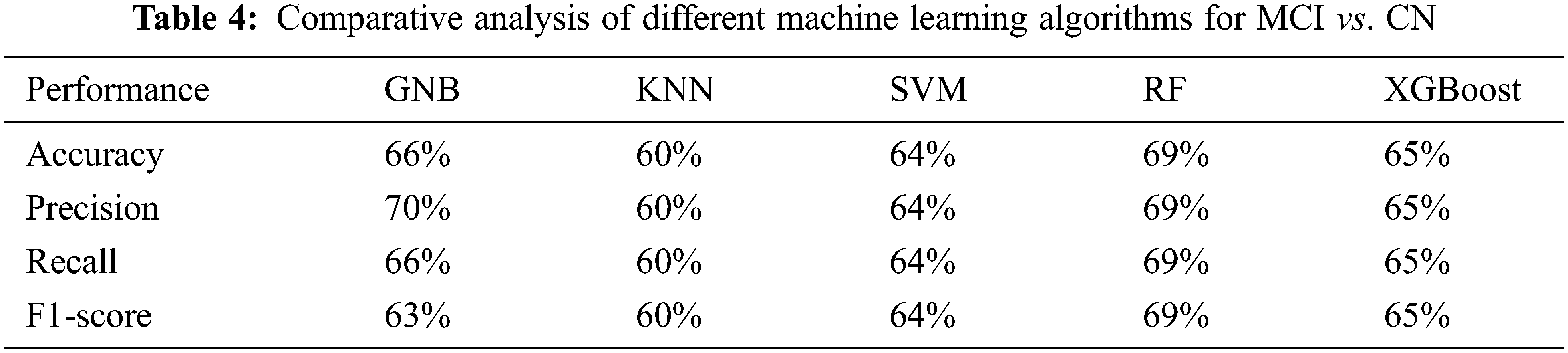

Figure 4: ROC for the classification of MCI and CN
In this paper, we calculated accuracy values for various numbers of trees (n_estimators) and it is observed that the best overall accuracy of 85% is obtained with a n_estimator value of 40, see Fig. 5. The best overall precision of 85% is obtained with n_estimator values of 40, see Fig. 6 below.

Figure 5: Accuracy for the prediction of Alzheimer’s with different number of trees

Figure 6: Precision for the prediction of Alzheimer’s with different number of trees
We calculated recall values for different numbers of trees (n_estimators) and it is observed that the best overall recall of 85% is obtained with a n_estimator value of 40, see Fig. 7. The best overall F1-score of 85% is obtained with n_estimator values of 40, see Fig. 8 below.

Figure 7: Recall for the prediction of Alzheimer’s with different number of trees
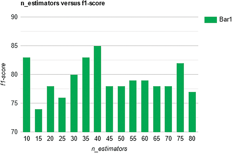
Figure 8: F1-score for the prediction of Alzheimer’s with different number of trees
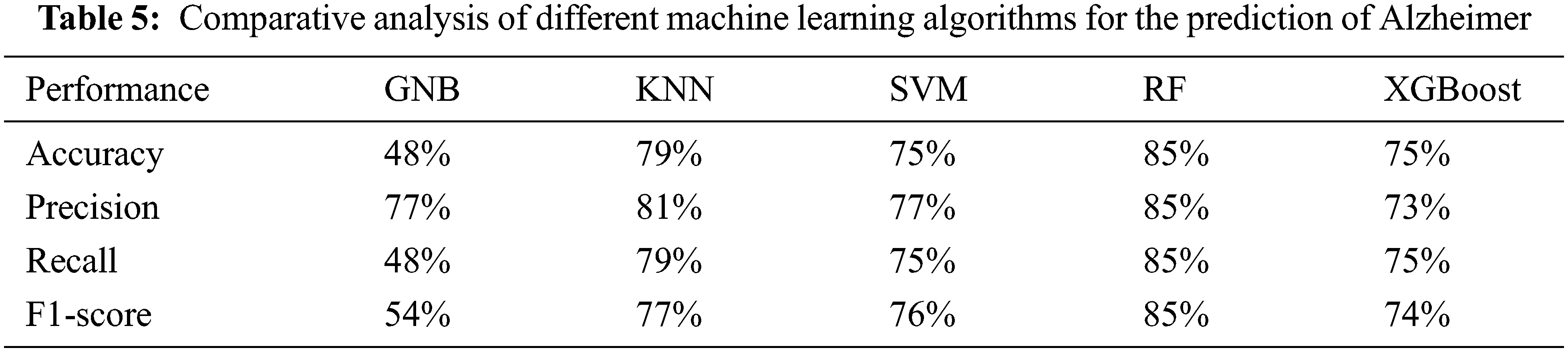
The proposed random forest-based approach with the Radiomic features achieved 85% accuracy recall, precision, and F1 score see Tab. 5. The proposed approach achieved 88% accuracy, 88% recall, 88% precision, and 87% F1-score for AD vs. CN, 72% accuracy, 73% recall, 72% precision, and 71% F1-score for AD vs. MCI and 69% accuracy, 69% recall, 68% precision and 69% F1-score for MCI vs. CN.
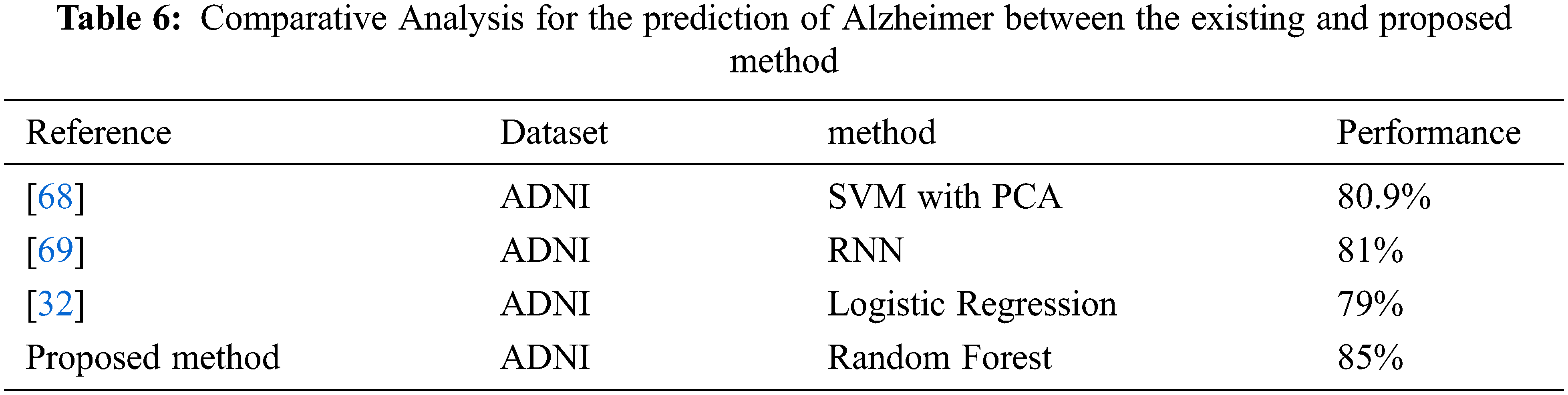
In the paper [68], the authors proposed SVM with PCA based method by using MR images and obtained an accuracy of 80.9%. In the paper [69], the author proposed RNN based method by using MR images and obtained an accuracy of 81%. The proposed approach of random forest classifier with the Radiomic features achieved the accuracy of 85% with taking parameter value as n_estimators = 40, criterion = ‘entropy’, random_state = 0. So based on the results proposed approach of random forest with Radiomic features gives better results for the prediction of AD at an early stage, see Tab. 6.
Alzheimer’s disease is a frequently occurring mental illness that occurs in about 60–80%, cases of dementia. Depending upon the severity of symptoms the patients can be categorized in CN, MCI, and AD. Machine learning algorithms that are used in this paper are SVM taking parameter values as kernel = ‘linear’, random_state = 42, K- Nearest Neighbour taking parameter values as n_neighbors = 5, metric = ‘minkowski’, p = 2, Gaussian Naïve Bayes, XGBoost as well as Random Forest Classifier. Random Forest with parameter n_estimators = 40, criterion = ‘entropy’, random_state = 0, provides best result in terms of Accuracy. The proposed random forest-based approach with the Radiomic features achieved 85% accuracy. The proposed approach achieved 88% accuracy, 88% recall, 88% precision, and 87% F1-score for AD vs. CN, 72% accuracy, 73% recall, 72% precision, and 71% F1-score for AD vs. MCI and 69% accuracy, 69% recall, 68% precision and 69% F1-score for MCI vs. CN. The comparative analysis shows that the proposed approach performed better than other existing approaches.
Funding Statement: The authors received no specific funding for this study.
Conflicts of Interest: The authors declare that they have no conflicts of interest to report regarding the present study.
References
1. S. Natarajan, S. Joshi, B. N. Saha, A. Edwards, T. Khot et al., “A machine learning pipeline for three-way classification of Alzheimer patients from structural magnetic resonance images of the brain,” in Proc. ICMLA, Florida, USA, pp. 203–208, 2012. [Google Scholar]
2. J. Gaugler, T. J. B. James, J. Reimer and J. Weuve, Alzheimer’s association, Wiley, Alzheimer’s disease facts and figures. In: Alzheimer’s Dementia. vol. 17. Chicago IL, USA, 20212021 [Google Scholar]
3. M. W. Bondi, E. C. Edmonds and D. Salmon, “Alzheimer’s disease: Past, present and future,” Journal of International Neuropsychological Society, vol. 23, no. 9, pp. 818–831, 2017. [Google Scholar]
4. B. J. Grabher, “Effects of Alzheimer disease on patient and their family,” Journal of Nuclear Medicine Technology, vol. 46, no. 4, pp. 335–340, 2018. [Google Scholar]
5. G. Serge, B. Reisberg, M. Zaudig, R. C. Petersen, K. Ritchie et al., “Mild cognitive impairment,” The Lancet, vol. 367, no. 9518, pp. 1262–1270, 2006. [Google Scholar]
6. K. A. Johnson, N. C. Fox, R. A. Sperling and W. E. Klunk, “Brain imaging in Alzheimer disease,” Cold Spring Harbor Perspectives in Medicine, vol. 2, no. 4, pp. a006213, 2012. [Google Scholar]
7. C. Pennanen, M. Kivipelto, S. Tuomainen, P. Hartikainen, T. Hänninen et al., “Hippocampus and entorhinal cortex in mild cognitive impairment and early AD,” Neurobiology of Aging, vol. 25, no. 3, pp. 303–310, 2017. [Google Scholar]
8. E. Fletcher, S. Villeneuve, P. Maillard, D. Harvey, B. Reed et al., “β-amyloid, hippocampal atrophy and their relation to longitudinal brain change in cognitively normal individuals,” Neurobiology of Aging, vol. 40, no. 4, pp. 173–180, 2016. [Google Scholar]
9. D. P. Devanand, G. Pradhaban, X. Liu, A. Khandji, S. De Santi et al., “Hippocampal and entorhinal atrophy in mild cognitive impairment: Prediction of Alzheimer disease,” Neurology, vol. 68, no. 11, pp. 828–836, 2007. [Google Scholar]
10. C. Zarow, L. Wang, H. C. Chui, M. W. Weiner and J. G. Csernansky, “MRI shows more severe hippocampal atrophy and shape deformation in hippocampal sclerosis than in Alzheimer’s disease,” International Journal of Alzheimer’s Disease, vol. 2011, no. 1, pp. 1–6, 2007. [Google Scholar]
11. M. Lustig, D. L. Donoho, J. M. Santos and J. M. Pauly, “Compressed sensing MRI,” IEEE Signal Processing Magazine, vol. 25, no. 2, pp. 72–82, 2008. [Google Scholar]
12. J. G. Stine, N. Munaganuru, A. Barnard, J. L. Wang, K. Kaulback et al., “Change in MRI-PDFF and histologic response in patients with nonalcoholic steatohepatitis: A systematic review and meta-analysis,” Clinical Gastroenterology and Hepatology, vol. 19, no. 11, pp. 2274–2283, 2021. [Google Scholar]
13. P. Thakare and V. R. Pawar, “Alzheimer disease detection and tracking of Alzheimer patient,” in Proc. Int. Conf. on Inventive Computation Technologies (ICICT), Coimbatore, India, vol. 1, pp. 1–4, 2016. [Google Scholar]
14. P. Telagarapu, B. Mohanty and K. R. Anandh, “Analysis of Alzheimer condition in t1-weighted MR images using texture features and k-nn classifier,” in Proc. Int. CET Conf. on Control, Communication, and Computing (IC4), Thiruvananthapuram, India, IEEE, pp. 331–334, 2018. [Google Scholar]
15. J. D. Lee, S. C. Su, C. H. Huang, W. C. Xu and Y. Y. Wei, “Using volume features and shape features for Alzheimer’s disease diagnosis,” in Proc. Fourth Int. Conf. on Innovative Computing, Information, and Control (ICICIC), Kaohsiung, Taiwan, IEEE, pp. 437–440, 2009. [Google Scholar]
16. S. Liu, H. Yang, L. Tong and W. Liu, “Detecting grey matter changes in preclinical phase of Alzheimer’s disease by voxel-based morphometric and textural features: A preliminary study,” in Proc. IEEE Third Int. Conf. on Information Science and Technology (ICIST), Yangzhou, China, pp. 30–34, 2013. [Google Scholar]
17. Y. Ding, C. Zhang, T. Lan, Z. Qin, X. Zhang et al., “Classification of Alzheimer’s disease based on the combination of morphometric feature and texture feature,” in Proc. IEEE Int. Conf. on Bioinformatics and Biomedicine (BIBM), Washington D.C., USA, pp. 409–412, 2015. [Google Scholar]
18. C. Ahmad, C. Desrosiers and T. Niazi, “Deep radiomic analysis of MRI related to Alzheimer’s disease,” IEEEAccess, vol. 6, pp. 55822–58213, 2018. [Google Scholar]
19. L. Yupeng, J. Jiang, T. Shen, P. Wu and C. Zuo, “Radiomics features as predictors to distinguish fast and slow progression of mild cognitive impairment to Alzheimer’s disease,” in Proc. 40th Annual Int. Conf. of the IEEE Engineering in Medicine and Biology Society (EMBC), Honolulu, HI, USA, pp. 127–130, 2018. [Google Scholar]
20. C. Ahmad and T. Niazi, “Radiomics analysis of subcortical brain regions related to Alzheimer disease,” in Proc. IEEE Life Sciences Conf. (LSC), Montreal, Quebec, Canada, pp. 203–206, 2018. [Google Scholar]
21. R. Usha and K. Perumal, “A modified fractal texture image analysis based on grayscale morphology for multi-model views in MR brain,” Indonesian Journal of Electrical Engineering and Computer Science, vol. 21, no. 1, pp. 154–163, 2021. [Google Scholar]
22. P. Telagarapu, K. R. Anandh and A. Sudhakar, “Classification of Alzheimer’s condition in T1-weighted MR images using GLCM and GLRLM texture features,” in Proc. of Int. Conf. on Wireless Communication, Singapore, Springer, pp. 533–541, 2020. [Google Scholar]
23. F. Feng, P. Wang, K. Zhao, B. Zhou, H. Yao et al., “Radiomic features of hippocampal subregions in Alzheimer’s disease and amnestic mild cognitive impairment,” Frontiers in Aging Neuroscience, vol. 10, pp. 290, 2018. [Google Scholar]
24. F. Qi, Y. Chen, Z. Liao, H. Jiang, D. Mao et al., “Corpus callosum radiomics-based classification model in Alzheimer’s disease: A case-control study,” Frontiers in Neurology, vol. 9, pp. 618, 2018. [Google Scholar]
25. O. W. Kadhim, “Alzheimer disease diagnosis using the K-means, GLCM and K_NN,” Journal of University of Babylon for Pure and Applied Sciences, vol. 26, no. 2, pp. 57–65, 2018. [Google Scholar]
26. Z. Jing, C. Yu, G. Jiang, W. Liu and L. Tong, “3D texture analysis on MRI images of Alzheimer’s disease,” Brain Imaging and Behavior, vol. 6, no. 1, pp. 61–69, 2012. [Google Scholar]
27. L. Sørensen, C. Igel, L. Hansen, M. Osler, M. Lauritzen et al., “Early detection of Alzheimer’s disease using MRI hippocampal texture,” Human Brain Mapping, vol. 37, no. 3, pp. 1148–1161, 2016. [Google Scholar]
28. J. Liu, J. Wang, B. Hu, F. X. Wu and Y. Pan, “Alzheimer’s disease classification based on individual hierarchial networks constructed with 3D texture features,” IEEE Transactions on NanoBioscience, vol. 16, no. 6, pp. 428–437, 2017. [Google Scholar]
29. L. Sorensen, C. Igel, A. Pai, I. Balas and C. Anker, “Differential diagnosis of mild cognitive impairment and Alzheimer’s disease using structural MRI cortical thickness, hippocampal shape, hippocampal texture, and volumetry,” NeuroImage Clinical, vol. 13, pp. 470–482, 2017. [Google Scholar]
30. R. Jayapathy, R. S. Moni and T. Gopalakrishnan, “Discrimination of Alzheimer’s disease using hippocampus texture features from MRI,” Asian Biomedicine, vol. 6, no. 1, pp. 87–94, 2018. [Google Scholar]
31. R. Sara, S. N. Velgos, A. C. Dueck, Y. E. Geda, J. R. Mitchell et al., “Brain MR radiomics to differentiate cognitive disorders,” The Journal of Neuropsychiatry and Clinical Neurosciences, vol. 31, no. 3, pp. 210–219, 2019. [Google Scholar]
32. A. M. Torteya, J. A. R. Rojas, J. M. C. Padilla, J. I. G. Tejada, V. Treviño et al., “Magnetization-prepared rapid acquisition with gradient-echo magnetic resonance imaging signal and texture features for the prediction of mild cognitive impairment to Alzheimer’s disease progression,” Journal of Medical Imaging, vol. 1, no. 3, pp. 031005, 2014. [Google Scholar]
33. P. Keserwani, V. C. Pammi, O. Prakash, A. Khare and M. Jeon, “Classification of Alzheimer disease using gabor texture feature of hippocampus region,” Int J Image Graphics Signal Processing, vol. 8, no. 6, pp. 13–20, 2016. [Google Scholar]
34. T. R. Sivapriya, V. Saravanan and P. R. J. Thangaiah, “Texture analysis of brain MRI and classification with BPN for the diagnosis of dementia,” in Proc. Int. Conf. on Computational Science, Engineering and Information Technology, Berlin, Heidelberg, pp. 553–563, 2011. [Google Scholar]
35. N. Surendran and K. V. Muneer, “Multistage classification of Alzheimer’s disease,” International Journal of Latest Technology in Engineering, Management & Applied Science (IJLTEMAS), vol. 6, pp. 199–204, 2017. [Google Scholar]
36. S. Rita, C. Slump and A. M. C. Walsum, “Using local texture maps of brain MR images to detect mild cognitive impairment,” in Proc. of the 21st Int. Conf. on Pattern Recognition (ICPR2012), Tsukuba, Japan, pp. 153–156, 2012. [Google Scholar]
37. P. Deekshitha, N. Madusanka, S. Bhattacharjee, H. G. Park, C. H. Kim et al., “A comparative study of Alzheimer’s disease classification using multiple transfer learning models,” Journal of Multimedia Information System, vol. 6, no. 4, pp. 209–216, 2019. [Google Scholar]
38. X. Zhou, Z. Liu, Z. Zhou and H. Xia, “Study on texture characteristics of the hippocampus in MR images of patients with Alzheimer’s disease,” in Proc. 3rd Int. Conf. on Biomedical Engineering and Informatics, IEEE, 2, pp. 593–596, 2010. [Google Scholar]
39. W. Xu, L. Z. Tong, X. Li, X. X. Zhou and H. F. Yang, “Study on texture features of cingulum in different gender patients with Alzheimer’s disease and mild cognitive impairment based on MR images,” in Advanced Materials Research, Switzerland, Trans Tech Publications Ltd., vol. 301, pp. 1060–1065, 2011. [Google Scholar]
40. Z. Pang, X. Wang, J. Qi, Z. Zhao, Y. Gao et al., “A multi-modal data platform for diagnosis and prediction of Alzheimer’s disease using machine learning methods,” Mobile Networks and Applications, vol. 26, no. 6, pp. 1–12, 2021. [Google Scholar]
41. X. R. Zhang, X. Sun, W. Sun, T. Xu and P. P. Wang, “Deformation expression of soft tissue based on BP neural network,” Intelligent Automation & Soft Computing, vol. 32, no. 2, pp. 1041–1053, 2022. [Google Scholar]
42. X. R. Zhang, J. Zhou, W. Sun and S. K. Jha, “A lightweight CNN based on transfer learning for COVID-19 diagnosis,” Computers, Materials & Continua, vol. 72, no. 1, pp. 1123–1137, 2022. [Google Scholar]
43. S. Manu, T. R. Aparna, P. R. Anurenjan and K. G. Sreeni, Deep learning-based prediction of Alzheimer’s disease from magnetic resonance images. In: Intelligent Vision in Healthcare, pages 145–151, 2022. [Google Scholar]
44. K. D. Jyoti, V. P. Singh and V. Kumar, “Two-way threshold-based intelligent water drops feature selection algorithm for accurate detection of breast cancer,” Soft Computing, vol. 26, no. 5, pp. 2277–2305, 2022. [Google Scholar]
45. T. Ashima, V. P. Singh and M. M. Gore, “Improved detection of coronary artery disease using DT-RFE based feature selection and ensemble learning,” in Proc. Int. Conf. on Advanced Network Technologies and Intelligent Computing, Varanasi, India, Springer, pp. 425–440, 2021. [Google Scholar]
46. V. Aman and V. P. Singh, “HSADML: Hyper-sphere angular deep metric based learning for brain tumor classification,” arXiv preprint arXiv, pp. 2201.12269, 2022. [Google Scholar]
47. S. Stephanie and R. Leahy, “Surface-based labeling of cortical anatomy using a deformable atlas,” IEEE Transactions on Medical Imaging, vol. 16, no. 1, pp. 41–54, 1997. [Google Scholar]
48. D. W. Shattuck, S. R. Sandor-Leahy, K. A. Schaper, D. A. Rottenberg and R. M. Leahy, “Magnetic resonance image tissue classification using a partial volume model,” NeuroImage, vol. 13, no. 5, pp. 856–876, 2001. [Google Scholar]
49. R. P. Woods, S. T. Grafton, J. D. Watson, N. L. Sicotte and J. C. Mazziotta, “Automated image registration: II. Intersubject validation of linear and nonlinear models,” Journal of Computer Assisted Tomography, vol. 22, no. 1, pp. 153–165, 1998. [Google Scholar]
50. D. E. Rex, J. Q. Ma and A. W. Toga, “The LONI pipeline processing environment,” Neuroimage, vol. 19, no. 3, pp. 1033–1048, 2003. [Google Scholar]
51. D. W. Shattuck and R. M. Leahy, “Automated graph-based analysis and correction of cortical volume topology,” IEEE Transactions on Medical Imaging, vol. 20, no. 11, pp. 1167–1177, 2001. [Google Scholar]
52. V. Griethuysen, J. M. Joost, A. Fedorov, C. Parmar, A. Hosny et al., “Computational radiomics system to decode the radiographic phenotype,” Cancer Research, vol. 77, no. 21, pp. e104–e107, 2017. [Google Scholar]
53. W. E. Lorensen, “History of the marching cubes algorithm,” IEEE Computer Graphics and Applications, vol. 40, no. 2, pp. 8–15, 2020. [Google Scholar]
54. R. M. Haralick, K. Shanmugam and I. H. Dinstein, “Textural features for image classification,” IEEE Transactions on Systems, Man, and Cybernetics, vol. SMC-3, no. 6, pp. 610–621, 1973. [Google Scholar]
55. T. Guillaume, B. Fertil, C. Navarro, S. Pereira, P. Cau et al., “Shape and texture indexes application to cell nuclei classification,” International Journal of Pattern Recognition and Artificial Intelligence, vol. 27, no. 1, pp. 1357002, 2013. [Google Scholar]
56. C. Sun and W. G. Wee, “Neighboring gray level dependence matrix for texture classification,” Computer Vision, Graphics, and Image Processing, vol. 23, no. 3, pp. 341–352, 1983. [Google Scholar]
57. A. Moses and R. King, “Textural features corresponding to textural properties,” IEEE Transactions on Systems, Man, and Cybernetics, vol. 19, no. 5, pp. 1264–1274, 1989. [Google Scholar]
58. M. M. Galloway, “Texture analysis using gray level run lengths,” Computer Graphics and Image Processing, vol. 4, no. 2, pp. 172–179, 1975. [Google Scholar]
59. A. Chu, C. M. Sehgal and J. F. Greenleaf, “Use of gray value distribution of run lengths for texture analysis,” Pattern Recognition Letters, vol. 11, no. 2, pp. 415–419, 1990. [Google Scholar]
60. D. H. Xu, A. S. Kurani, J. D. Furst and D. S. Raicu, “Run-length encoding for volumetric texture,” Heart, vol. 27, no. 25, pp. 452–458, 2004. [Google Scholar]
61. N. Tustison and J. C. Gee, “Run-length matrices for texture analysis,” Insight J, vol. 1, pp. 1–6, 2008. [Google Scholar]
62. X. Tang, “Texture information in run-length matrices,” IEEE Transactions on Image Processing, vol. 7, no. 11, pp. 1602–1609, 1998. [Google Scholar]
63. C. Padraig and S. J. Delany, “k-Nearest neighbour classifiers-A tutorial,” ACM Computing Surveys (CSUR), vol. 54, no. 6, pp. 1–2, 2021. [Google Scholar]
64. W. S. Noble, “What is a support vector machine?,” Nature Biotechnology, vol. 24, no. 12, pp. 1565–1567, 2006. [Google Scholar]
65. C. Tianqi, T. He, M. Benesty, V. Khotilovich, Y. Tang et al., “Xgboost: Extreme gradient boosting,” R Package Version 0.4-2, vol. 1, no. 4, pp. 1–4, 2015. [Google Scholar]
66. G. Biau and E. Scornet, “A random forest guided tour,” Test, vol. 25, no. 2, pp. 197–227, 2016. [Google Scholar]
67. M. Belgiu and L. Drăguţ, “Random forest in remote sensing: A review of applications and future directions,” ISPRS Journal of Photogrammetry and Remote Sensing, vol. 114, no. Part A, pp. 24–31, 2016. [Google Scholar]
68. J. E. Arco, J. Ramírez, J. M. Górriz, M. Ruz, Alzheimer’s Disease Neuroimaging Initiative, “Data fusion based on searchlight analysis for the prediction of Alzheimer’s disease,” Expert Systems with Applications, vol. 185, no. 1, pp. 115549, 2021. [Google Scholar]
69. L. Garam, K. Nho, B. Kang, K. A. Sohn and D. Kim, “Predicting Alzheimer’s disease progression using multi-modal deep learning approach,” Scientific Reports, vol. 9, no. 1, pp. 1–12, 2019. [Google Scholar]
Cite This Article
 Copyright © 2023 The Author(s). Published by Tech Science Press.
This work is licensed under a Creative Commons Attribution 4.0 International License , which permits unrestricted use, distribution, and reproduction in any medium, provided the original work is properly cited.
 Downloads
 Citation Tools