Software Defect Prediction Based Ensemble Approach

1  Introduction

Software testing becomes more demanding as the number of software applications expands. Finding potential defects among millions of code lines and thousands of documents is a difficult task for a software tester [1]. However, finding as many errors as feasible is vital to improving software quality, particularly in some critical scenarios where even a minor undiscovered software failure might have devastating effects [2,3]. Software fault prediction which is entrenched in static code features and can lead engineers to discover problem-prone modules earlier instead of random inspection in the sector has drawn increasing interest from researchers in recent years [4–6]. Modern software systems are huge and complex, containing several interconnected components or modules. Additionally, in adapting to variations in system needs or user expectations, these software applications are continuously upgraded and expanded with new features or functionalities [7]. A range of software metrics (mechanisms) with varied capacities can be used to assess the quality of these sophisticated software systems [8]. As an outcome, the number of software features produced is frequently considerable, resulting in a high-dimensionality issue [9]. The excessive dimensionality of software features, according to several previous studies, is often the reason for SDP models’ poor predictive accuracy. The presence of unnecessary and duplicated software measurements, in other words, has a negative impact on SDP model performance [10–12].

Another issue is high dimensionality, which is brought on by software metrics. SDP models were developed using a variety of software metrics (also known as features), including static code metrics, process metrics, and so on [13]. Software measurements obtained from software entities are generally redundant and correlative, which might have a negative impact on the model’s SDP effectiveness [14]. Feature selection and feature extraction strategies have been demonstrated to aid with this issue in earlier SDP research. However, when contrasted to deep features collected by deep learning, practically all of these measurements are classical metrics [15]. Although numerous classifiers have been employed for defect prediction, they discovered that most defect prediction classifiers function similarly [16]. As a result, additional characteristics like computing efficiency and simplicity should be considered when selecting classifiers for defect prediction. Furthermore, in defect data, there is often a class imbalance, with non-faulty modules outnumbering defective modules. As a result, most classifiers categorize minority samples as majority samples. The train-set was created using a Double Transfer Boosting (DTB) technique, which allowed for the building of an effective SDP model with fewer data using cross-company data. Their approaches could potentially add new sample redundancy to the training data. It employs a feature matching technique to boost Area Under Curve (AUC) accuracy by turning heterogeneous features into paired features [17].

Machine learning (ML)-based algorithms, such as Random Forest (RF), Bayesian and Logistic Regression (LR) are the most popular and fascinating in the recently published literature on SDP, and these approaches have been demonstrated to be beneficial for detecting defect-prone modules [18]. Regrettably, there is still a serious issue to be resolved: In nature, software defect datasets have a class imbalance, meaning that defective instances make up a tiny percentage of the data whereas the majority of software modules are defect-free. Working with data that has an imbalanced class distribution presents a significant barrier for most standard classification techniques [19].

Existing defect prediction approaches, on the other hand, did not adequately address this issue, resulting in poor performance [20]. Even though these tactics are unique and well-thought-out, their inefficiency makes meeting the software industry’s rising needs difficult.

We present a novel hybrid classification strategy that integrates a Deep Neural Network (DNN) with a Multilayer Preceptor (MLP) model in this research. The ability to increase a prediction model’s performance is mostly dependent on two major factors: feature representation and categorization. We intend to find an effective classifier with improved performance for every software project, as well as a strong distinguishing feature representation. The EMWS method is used to choose features, and the classification is done using a hybrid technique.

The following are major contributions of this research work:

•   Hybrid of Whale Optimization Algorithm (WOA) and Firefly Algorithm (FA) (EMWS) is an upgraded metaheuristic feature selection algorithm based on the recently proposed WOA and another complementing FA algorithm. The strong global search WOA is used to improve the weak exploration of the FA algorithm.

•   To the best of our knowledge, feature selection in Software Defect Prediction (SDP) uses a hybrid exploration-focused algorithm based on population and an exploitation-oriented approach based on single-solution.

•   We construct a hybrid approach DNN and MLP based classification scheme.

•   EMWS algorithm for feature selection and hybrid approach for classification can achieve superior prediction performance.

The remainder of this paper is organized as follows: Section 2 discusses the related work. Sections 3 and 4, go over the background and proposed method in depth. Threats to validity are discussed in Section 5. In Section 6, we report the results of the performance verification experiments. The final section of the article concludes the work and discusses future directions in Section 7.

2  Literature Review

Chen et al.[21] suggested the Collective Training mechanism for Defect Prediction (CTDP), which divides into two parts adaptive weighting phase and the source data expansion phase. The Particle Swarm Optimization (PSO) technique was used by CTDP to fully consider all of the source projects to predict the target project. To begin, they employ a variety of normalization techniques to capture various aspects of source projects. Second, use an adaptive weighting mechanism to fully incorporate the data into a collective classifier for superior prediction outcomes. In the past, one-to-one Cross Project Defect Prediction (CPDP) was always presented using transfer learning techniques.

Qiu et al. [22] introduced the Transfer Convolutional Neural network (TCNN) method first parses the source file into integer vectors as the network inputs. The TCNN technique was then created by adding a corresponding layer to the Convolutional Neural Network (CNN), which integrated the hidden presentations of the source and target project-specific data into a reproducing kernel Hilbert space for distribution matching. The developed TCNN should extract transferrable DL-generated features by simultaneously decreasing classification error and distribution divergence among projects. It was demonstrated that the TCNN method outperformed the benchmark models.

Qiao et al. [23] suggested the DL method in which the number of defects is predicted. A publicly available dataset was pre-processed, including log transformation and data normalization. The data input for the deep learning model was then prepared using data modeling. Then, to anticipate the number of errors, feed the modeled data into a specifically developed DNN-based model. They test the proposed method on two well-known datasets. The defined method lowered the mean square error by a significant amount on average.

Tong et al. [24] presented stacked denoising autoencoder (SDAE) and two ensemble learning. To tackle the class-imbalance problem, researchers first used SDAEs to extract the deep representations (DPs), and then proposed TSE, a hybrid learning method. F-measure, AUC, and Matthews’ correlation coefficient (MCC) were used to assess the performance. When compared to benchmark SDP models, classic ensemble methods, and traditional metrics, DPs, d two-stage ensemble (TSE), and SDAEs TSE all lead to much higher performance. For SDP, SDAE is a powerful tool.

Hybrid multi-objective cuckoo search under-sampled software defect prediction model based on SVM (HMOCS-US-SVM) was introduced by Cai et al. [25]. To choose non-defective sampling and improve the parameters of SVM, an ensemble multi-objective Cuckoo Search (CS) with HMOCS was used. Then, to pick the non-defective modules, three under-sampled decision area range approaches were provided. The performance of the provided algorithm was measured in the simulation using three indicators: G-mean, false positive rate (pf), and probability of detection (pd). The suggested SDP model greatly improved SDP representation, according to the results of the experiments.

Zhu et al. [26]. employed kernel twin support vector machines (KTSVMs) to construct domain adaptation (DA) to fit the distributions of training data. The CPDP method was formulated using the KTSVM. The experimental results showed that in most circumstances, the suggested CPDP model outperforms the benchmark CPDP model in terms of predictive accuracy.

Gated hierarchical long short-term memory networks (GH-LSTMs) was introduced by Wang et al. [27] to predict the defects. The hierarchical LSTMs architecture allows GH-LSTMs to extract both semantic and conventional characteristics at the same time. Under non-effort-aware cases, the findings suggest that the suggested GH-LSTMs approach performs better approach in terms of F measure.

Balogun et al. [28] proposed the adaptive rank aggregation-based ensemble multi-filter feature selection (AREMFFS) approach to deal with the problem of large dimensionality and filter rank selection in SDP. The empirical outcome demonstrates the model’s efficiency over existing approaches.

An efficient binary variant of MFO (BMFO) was presented by Khurma et al. [29]. After a certain number of iterations, a migration step is done to trade solutions between islands, increasing the algorithm’s diversity power. The experiment findings suggest that FS enhances the categorization result.

CNNs were introduced by Nevendra et al. [30]. to detect faults in software modules. The CNN method is then trained using the provided metrics, and once trained, it can predict the defective occurrences. The suggested technique outperforms Li’s CNN and a typical Machine Learning model, according to experimental findings.

3  Background

By building an effective prediction model, SDP seeks to identify probable problems in new software modules in advance. However, the model’s performance is degraded by features that are both redundant and unnecessary. Feature selection (FS) is a crucial phase for redundant features. The fundamental issue of FS techniques is in determining the appropriate subset of features to reflect the original data properly. However, FS is a search issue in which each point in the search area represents a subset of features. A three-element binary array can be used to express a feature subset if a dataset has three features, such as (A, B, C). If the value of an element is 1, that feature is included in the feature subset; if the value is 0, that feature is not selected. As a result, (1, 1, 1) denotes that all three features have been chosen, whereas (0, 1, 0) denotes that only the second feature has been chosen. Large problems are difficult to tackle with an exact search strategy because FS is a nondeterministic polynomial time (NP)-hard issue. If the dataset has n features, for example, 2n subsets will be constructed and evaluated. As a result, heuristic search algorithms are frequently used as a substitute for reducing processing costs.

4  Methodology

In our proposed method it consists of three modules pre-processing, FS and defect prediction using an ensemble classifier. In the first step, we pre-process the software module. The repeating entities can then be eliminated, with the missing values being replaced. Normalization occurs after pre-processing. Normalization of datasets is a crucial preprocessing step for achieving high accuracy and learning speed. The WOA and the FA have been used to improve the EMWS algorithm for feature selection, which can choose less but closely connected representative features. The selected characteristics are then categorized using the proposed ensemble learning method. We begin by extracting the deep representation from the casual software metric using a MLP. Furthermore, using an adaptive Auto Encoder (AE), the categorization is done in a DNN. The performance of the classifier is improved by adding to this MLP.

Fig. 1 depicts the overall framework of the proposed approach.

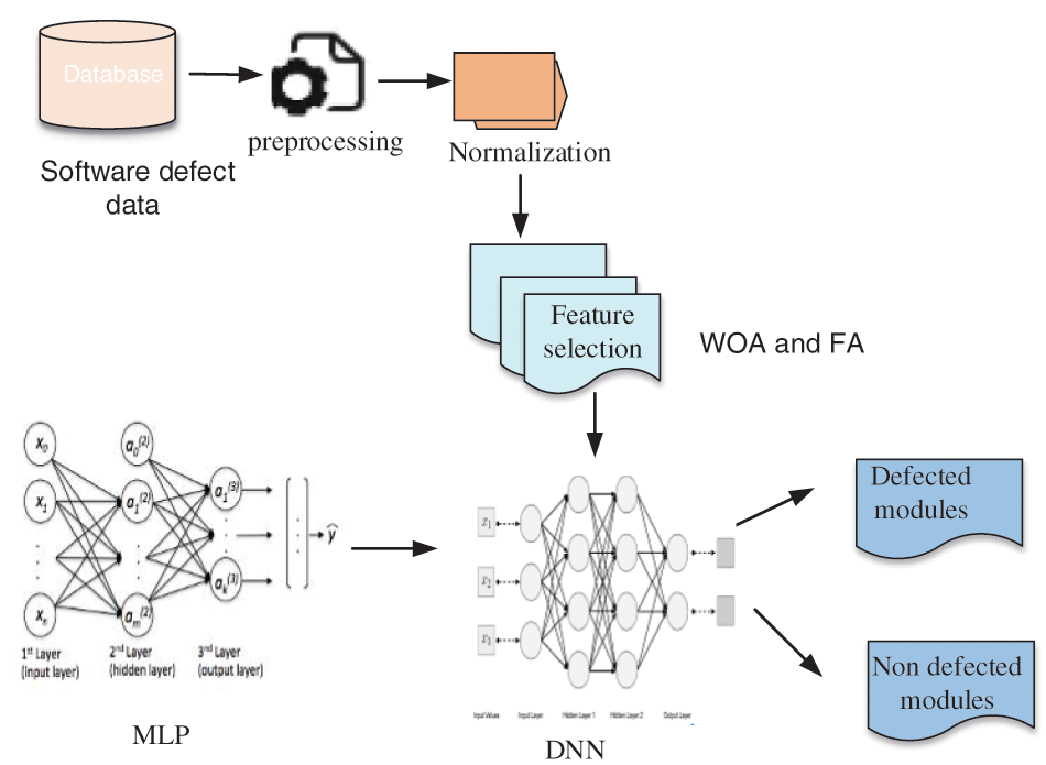
Figure 1: Architecture diagram of the proposed approach

4.1 Preprocessing

4.1.1 Deletion of Duplicated Modules

Pre-processing is used to determine the total number of software defect number modules and to eliminate similar modules from data sets. To be more exact, duplicate instances will generate overly optimistic results if they are routinely separated into a subset of the test data; otherwise, they will produce an unduly pessimistic outcome. Furthermore, they do not just slow down the training process, but they have minimal impact on the model’s efficiency. As a result, any redundant modules should be eliminated.

4.1.2 Replacement of Missing Values

If an entity has one or more missing values, it will not be able to fully satisfy our method input requirements. These missing values must be filled in. In this research, we substitute the mean of the related statistic for missing values. This strategy is proposed, in which the average of the related metric is utilized to replace a missing value. Assume that a metric mt and its observation {mt1,mt2,mt3,…..,mt100} suppose mt99 and mt100 are both missing. These two missing values are filled in using

mt99=mt100=198∑i=198mti (1)

4.1.3 Data Normalization

We normalize the experimental data for the convenience of testing and operation because most software measures are in various orders of magnitude. For good accuracy and quick learning, the normalization method is applied. On these measures, we do data normalization on values of varying magnitudes. In this research, we use the most common minimal maximum normalization approach to normalize the data. The minimum and maximum values of a measure x are represented by a min of (x) and a max of (x) respectively.

x~i=xi−min(x)max(x)−min(x) (2)

4.2 Feature Selection

In this paper, we incorporate an updated metaheuristic FS optimization algorithm by combining the powerful unique qualities of the WOA and FA. We use FF’s strong local exploration capability to improve the WOA’s weak exploitation efficiency, and WOA’s strong global navigation capability to improve Firefly’s weak exploration to a substantial measure synchronously, resulting in better search efficiency than if they used each of them individually in the FS issue of fault prediction. We use the WOA algorithm to discover the best global solution, then the FA to find the best solution based on the best solution already obtained, and so on in an iterative cycle. This is because WOA’s solution would be insufficient after a certain number of iterations, or the exploration would become imprisoned in the local optimum, whereas FA on the other hand, accepts inferior methods with a certain degree of probability and can escape the local optimum.

4.2.1 Whale Optimization Algorithm (WOA)

The WOA method is a metaheuristic algorithm based on stochastic populations that mimics humpback whales’ intelligent foraging behavior when using bubble-net feeding. That moves toward a pray spot that produces the best location like a group of whales. Because WOA is a population-based algorithm, the starting population must be generated initially.

The WOA consists of two-stage, that is

1. Exploitation stage

2. Exploration stage

Humpback whales apply the method of their location in reaction to the location of the prey during this phase of the hunt. The current best candidate solution, according to the WOA, is the target prey’s position or the position closest to it. The movements of whales to their prey are equivalent to the operation of estimating fitness value to locate the best feature subset in the context of SDP.

The following are the mathematical equations for this process:

D→=|V→.Y∗→(c)−Y→(c)| (3)

Y→(c+1)=Y∗→(c)−B.→C→ (4)

While current iteration is indicated as t, X∗→ represents the current solution, Y→(s+1) and indicates the target coordinate vector after the next iteration.

B→ and c→ are coefficient vector

B→=2n→.t→−n→ (5)

V→=2t→ (6)

where the variable n→ starts at 2 and decreases linearly to 0 over several rounds, and a variable t→ is a random number among 0 and 1, created by a uniform distribution function. When exploring in n-dimensional space, Eqs. (3) and (4) Allow the WOA to outperform the competition.

Y→(c+1)=C2→.ebl.cos⁡(2πl)+Y∗→(r) (7)

C2→=|Y∗→(r)−Y→(r)| (8)

While D2→ representing the distance between the humpback whale’s present position and the current ideal individual. Constant is denoted by I, and l is a random value in between [1,1].

Y→(r+1)∗=|Yr∗−Y(r)|→.eir.cos⁡(2πl)+Y→(r)∗ (9)

They estimated a 50% likelihood of selecting one of them to upgrade the position of whales throughout the process to replicate both the diminishing encircling method as stated in Eq. (10):

{Y→(r+1)=Y∗→(r)−B→.C1→when m<0.5Y→(r+1)=C2→.eir.cos⁡(2πl)+Y∗→(r)when m≥0.5 (10)

The exploration for prey (exploration phase) can involve the whales conducting a worldwide search for a randomly selected agent. When the random value is more than 1 or less than 1, this technique is employed. Equations that can be used to represent the hunt for prey include:

C→=|D→..Y→rand−Y→| (11)

Y→(r+1)=Y→rand−B→.C→ (12)

The fitness evaluation values for the solution are given as binary numbers. The fitness function employed is often suited to the classification representation and the number of attributes chosen. That is demonstrated using the following calculation (10):

fθ=α.H+(1−α)∑iθiF (13)

4.2.2 Firefly Algorithm (FA)

FA is an up-to-date search and optimization tool. Its origins can be traced back to the flashing activity of fireflies. When differentiated from normal distributed arbitrary searches, Fireflies interact with one another through bioluminescent shining, which allows them to explore the cost-function space significantly more effectively. The light of the fireflies attracts them to others. The protocol’s fundamental rules are as follows:

•   The gender of each Fireflies should be similar.

•   If there are one or many fireflies, the Fireflies with the lesser light is drawn to the Fireflies with the brighter light.

•   When there are no brighter fireflies, they will fly wherever they want.

Light Intensity as Well as Attractiveness

The attractiveness of this Fireflies will be determined by two factors: a change in the intensity of light and the attractiveness formulation. The brightness of this Fireflies will be analyzed in terms of the objective function that must be optimized, and its brightness will determine the attractiveness among the fireflies that correspond to this.

As a result, light intensity K(t) differs according to the inverse square law in its most simple form.

K(t)=Kst2 (14)

The intensity of the light K differs with the space t, which has an absorption coefficient, as indicated scientifically in the formula:

I=I0e−γr (15)

For ignoring singularity at t = 0 in the equation Ks/t2, the collate effect of the inverse square law and absorption can be represented as the Gaussian type illustrated in Eq. (16)

I=IOe−γr2 (16)

The attractiveness β of a FA is related to the brightness noticed by nearby fireflies, as shown in Eq. (17):

β=β0e−γr2 (17)

At r = 0, βo denotes the attraction. Because computing (1 + r2) is faster than computing an exponential function, the function can be estimated as indicated in Eq. (18):

β=βo(1+γr2) (18)

Characteristic distance is defined in (16) and (17) that is 1/γ over which the attractiveness is changing considerably from βo to βoe−1 for (16) or βo/2 for (17). In real-time execution, β(r) consists of the attractiveness function that may be any monotonically minimizing function as in Eq. (19):

β(r)=βoe−γrm(m≥1) (19)

The typical length of a fixed is defined by Γ=γ−1x→1,x→∞

Conversely, γ may be utilized as the generic initial value for a particular length scale Γ in an optimization problem, i.e., γ=1tx

The Cartesian distance model is used to determine the distance between any two fireflies.

tuv=||xu−xv||=∑k=1a(xiuk−xvk)2 (20)

This FA fitness function improves efficiency in a testing set of training data while preserving the sufficient sample number chosen, as in Eq. (21).

fθ=ω∗E+(1−ω)∑iθiN (21)

In which fθ signifies the fitness function that is applied to an N-dimensional vector. The amount of characteristics in a data set is N, the categorization rate of inaccuracy is E, and the performance of the classifier is constantly controlled by the features picked. αt+1=αt∗δ

In which δ is the absolute rate of expansion in the case of the randomization factor, and t is the randomization factor at iteration t.

The EMWS technique considers two optimization objectives when it comes to feature selection in the SDP. Decreasing the number of selected characteristics is one optimization aim while lowering classification error is another. The fewer features are chosen and the lesser the classification error, the greater the response.

We use the below function to examine the solution in the EMWS method in this paper:

fitness=λμ|c|(LR)+ω|C||N| (22)

where μ|D| (KJ) indicated the classification error. To achieve greater performance than employing each one independently, the distinctive qualities of SA and WOA can be combined into an ensemble metaheuristic algorithm.

4.3 Multilayer Preceptor (MLP) for Performing Defect Prediction

Forward neural networks (FNNs) are fed multilayer perceptron neural networks that have been trained using the usual Back propagation (BP) algorithm. MLPs are frequently utilized for modeling prediction problems because they can be taught to learn how to transform incoming data into a desirable response. The MLP is a supervised learning artificial neural network that has been used to solve a variety of issues, involving pattern recognition, identification, classification, control systems, vision, and speech. MLP is mostly utilized in seismic activity prediction for information processing and pattern identification.

The characteristics are the network’s inputs, which are weighted and sent to the first hidden layer at the same time.

Z−inj=voj+∑i=1nxivij (23)

The weighted outcome of the last hidden layer, which is sent into the final layer, is used to reveal the network’s prediction for specific tuples.

y−ink=wok+∑j=1pziwjk (24)

Every output unit adds up its weighted input signal, which is represented as

Yk=f(y−ink)1 (25)

Every output unit ( xm,m=1,……,n) getting a target pattern corresponding to an input pattern error information term is evaluated as

δk=(rk−zk)f(z−ink) (26)

Every hidden unit (zj,j=1,….,p) sums its delta inputs from units in the layer above

δ−nmk=∑m=1nδiWjk (27)

The term for information of error is computed as follows:

δj=δ−injf(z−inj) (28)

The weights are adjusted using back-propagation from the output layer to the first hidden layer to minimize the mean error among the actual and predicted values.

Every output unit upgrades its bias and weight j = (0… h) thus it is represented as

fuv(r+1)=fuv(t)+αδkki+μ[fuv(r)−wuv(r−1)] (29)

where α are learning rate and l is momentum factor updates its bias and weight i = (0… m)

This accepts the weighted inputs and transmits data from the previously hidden layer to the next. For each buried layer, various activation functions are differentiated. Sigmoid has been employed as the output layer. It has been discovered that MLP with a single hidden layer performs better.

4.4 Deep Neural Network (DNN)

The DNN approach is used for software defect classification and prediction. This method is beneficial for identifying traits that are both effective and discriminative. For immense quantities of unlabelled data, DNN can be used. Because our research focuses on SDP, which is a challenging task, pattern learning becomes more complicated. To address this problem, we describe an enhanced DNN based on sparse autoencoders (SAE). Adaptive AE is combined with a de-noising approach in the proposed method to learn the characteristics. These learned properties are also put into a neural network classifier. The following subsections detail the entire procedure of the proposed approach.

4.4.1 Adaptive Auto Encoder (AE)

A technology known as an AE is an asymmetrical type of neural network. For feature learning on large datasets, AE are employed. By lowering training error and minimizing the loss function, AE give a tremendous performance. The primary goal of an AE is to recreate input data perfectly at the output layer. Traditional encoders are fault in that they replicate the input layer to a hidden layer, which distorts critical input data information. We describe an enhancement to the classic AE that improves the system’s performance in this study.

let us consider that input dataset I include M × N dimension which is estimated as X = {y(1), y(2),………y(i),……y(S)} ∈EN . The length of the dataset is M, and the amount of samples evaluated is N. The selection of the activation function is a major step in this technique that affects the outcome. We chose the sigmoid activation function for our research because of its importance in improving performance.

The next stage in this method is to implement feature learning and comprehend the expression of features on input data, which is referred to as un-labeled data in this case. This phrase is represented as follows:

k(y(j),S,a)=σ(Sy(j)+a),j=1,..,M) (30)

The output layer function is represented as

output_layer=σ(STg(y(j),S,a)+v) (31)

We also employ an objective function, which reduces the recurrence of input features. This phrase is used on the hidden layer to control the active neurons at the time of the iteration. Consider the activation function of the jth hidden layer, which is a j (x).

This approach is used on the feature input set X, with the hidden layer expressed as Eq. (31).

a=sigmoid(SY+a) (32)

The average activation function is thought to be near 0 because the neurons are dormant at the start of DNN training. If the average activation function varied from its significant value, we penalized it. The following is a summary of the situation:

Ppenalty=∑j=1s2KL(ρ||ρj) (33)

KL (.) is the Kullback–Leibler divergence, and s2 is the overall amount of neurons available in the buried layer. This difference can be represented in the following way:

NM(ρ||ρj)=ρlogρρj+(1−ρ)log1−ρ1−ρj (34)

If ρj=ρthen KL(ρ||ρj)=0 otherwise, it maintains an increment that produces divergence, which is referred to as the adaptive constant. This can be calculated using the following cost function:

Cadaptive(W,b)=ℓ(W,b)+β∑j=1s2KL(ρ||ρj) (35)

The process of identifying significant parameters b and W is critical since the cost function and these two parameters are directly related to every another, affecting system performance. As a result, we propose an optimization problem to tackle this, intending to decrease the adaptive cost (b, W). This optimization issue can be tackled utilizing a BP strategy, which involves iteratively updating W and b. It is expressed as:

Suv(k)=Suv(k)−ϵ∂∂Suv(k)Xadaptive(S,a) (36)

And

aj(k)=ak(K)−ϵ∂∂ai(l)Xadaptive(S,a)

ϵ - indicates the learning rate of the DNN method.

4.4.2 Denoising for Adaptive Auto Encoder (AE)

The adaptive AE denoising approach is discussed with the use of de-noise coding, this technique can produce a better representation of a feature. The adaptive AE method to de-noising is described. This method offers a partially broken input pattern to the input data pattern to initialize the deep structures. This approach can generate a better representation of a feature by using de-noise coding.

q0(Y,Y,f)=q0(Y)qC(Y|X)∂f0(x)(x) (37)

∂f0(y)(x)is set to 0 if f0(x)≠y.q0(X) (38)

This symbol represents the likelihood function of the input training dataset. The objective function is to recreate the input corrupted pattern, which may be expressed as follows:

argθ,θ′min⁡Eq0(x,x)[L(x,x′)] (39)

L(Y, Y)) represents the reconstruction error. If a short dataset is used for evaluation during the data training process called “overfitting” error occurs, degrading the training representation and outcomes in reduced classification accuracy. To solve the problem, we use an Eq. (39) and set the output of neurons to zero, indicating that they will not participate in the propagation stage. This approach aids in the reduction of feature extraction or selection errors, as well as the improvement of classification accuracy.

5  Threats Validity

Massive investigative learning has been controlled in this research, and several possible risks to validity should be obtained. In our outcome, the prediction model poses a significant threat.

This entails deciding on performance requirements for calculating defect model prediction. We handle these metrics since they were often utilized in previous research.

5.1 Internal Validity

The internal validity of this learning necessitates the duplication of the computing technique as well as the parameters of the fault prediction models. Internal validity threats are most often related to dissatisfaction and selection bias, which point to the experiments’ possible shortcomings. It is concerned with several unregulated internal elements that may have an impact on the outcomes. Apart from that, we have double-checked all of our research, but there are some inaccuracies.

5.2 External Validity

External validity is a ratio that determines how to examine outcomes that will be applied to the subject under study and another investigation. On five publicly available datasets, we test the proposed method. As a result, the recommended strategy provides the best solution.

5.3 Construct Validity

The term “construct validity” refers to the accuracy with which assessment indicators are projected. Threats to concept validity may interact with the data quality of datasets utilized in investigative studies. Probability of detection, positive rate, and G-mean to class imbalance defect dataset and balance, which may be employed repeatedly in SDP, are three popular measures that can be carefully selected. To reduce the threads, AUC was used to measure the projection model’s success. In today’s SDP, the representation metric is commonly utilized. Massive investigative learning has been controlled in this research, and several possible risks to validity should be obtained. In our outcome, the prediction model poses a significant threat. This entails deciding on performance requirements for calculating defect model prediction. We handle these metrics since they were often utilized in previous research.

6  Experimental Simulation

Experimental learning may be described in the proposed learning hybrid approach, and fault software prediction can be transferred. For software fault classification and prediction, a hybrid approach employing DNN and MLP is used with the MATLAB tool. We look for software defects in the data set repository as PROMISE.

6.1 Dataset

Throughout this study, we will utilize five SDP datasets: JM1, MC2, PC1, KC2, and KC3. These datasets will be used to apply prediction in Software fault models and will be used to confirm the Prediction of Software fault models. The public PROMISE repository datasets, which are commonly utilized in empirical research of Software fault Prediction, are now available. The database is generally used to test datasets and anticipate defects, and it has a variety of class imbalance ratios. To give a comparative review to emphasize the importance of the proposed ensemble method. In the software dataset, several general attributes are represented. Tab. 1 displays the dataset’s information and characteristics names.

6.2 Performance Indicator

The performance of a binary classifier prediction method is approximated using a confusion matrix, which is significant and noteworthy for efficiency evaluation. As a result, we may compute the following performance metrics:

True positive (TP): represents the amount of defect-prone modules appropriately anticipated as such.

True negative (TN): The amount of defect-free modules correctly anticipated as defect-free.

False-negative (FN): The number of modules that are defect-prone but are wrongly forecasted as defect-free.

False-positive (FP): The amount of defect-free modules wrongly categorized as defect-prone.

Accuracy: It’s a statistic for modules that have been appropriately categorized. In terms of the total number of modules in a software project, there is a clear separation between defect-prone and defect-free modules. It’s explained in Eq. (40)

Accuracy=(TP+TN)(TP+TN+FP+FN) (40)

Precision: It’s estimated by multiplying the amount of successfully categorized defect modules by the proportion of false-positive and true-positive defect modules. This is demonstrated in Eq. (41)

Precision=TP(FP+TP) (41)

Sensitivity: It’s evaluated by dividing the total amount of defect modules in the dataset by the amount of potentially categorized defect modules. It’s calculated in Eq. (42)

sensitivity=TP(FN+TP) (42)

False-positive rate (FPR): It’s calculated by dividing the total amount of non-defective modules by the number of incorrect positive predictions in the dataset. This is demonstrated in Eq. (43)

FPR=FP(TN+FP) (43)

True-negative rate: Specificity is another term for it. The accurate classification rate is defined as the percentage of rightly categorized negative predictions out of the overall amount of negative predictions. It’s shown in Eq. (44).

TNR=TN(FP+TN) (44)

F-Measure: It’s the average of precision and sensitivity, as shown in Eq. (45)

F−Measure=2×precision×sensitivityprecision+sensitivity (45)

The comparison of the suggested approach to the proposed model is depicted in the following Tab. 2.

Tab. 2, shows the representation of the JM1 dataset’s various performances compared with the existing approaches. The proposed approach value is indicated in black fonts. The evaluation of the proposed method is shown in Fig. 2, achieves a greater result in that dataset. When compared with other techniques our proposed approach gains a higher solution.

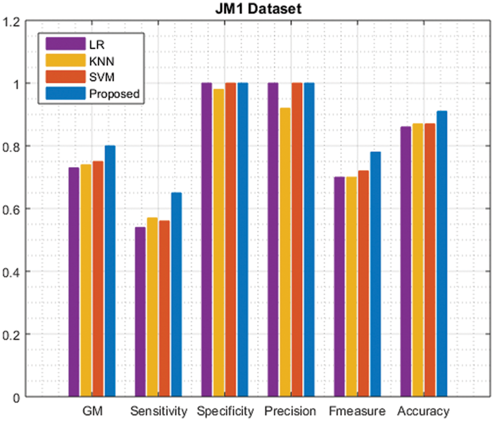
Figure 2: Comparison of JM1 dataset performance with the existing approach

Tab. 3 compares the performance of the KC2 dataset to that of the existing method. The proposed approach value is highlighted.

Fig. 3 shows that the evaluation of the hybrid approach achieves a higher result. The findings indicate that the recommended strategy produces promising results.

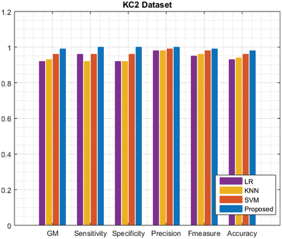
Figure 3: Comparison of KC2 dataset performance with the existing approach

Tab. 4 and Fig. 4 show the comparison of PC1 dataset performance with the existing approach. Where our proposed approach yields a better result compared with the existing approach.

Figure 4: Comparison of PC1 dataset performance with the existing approach

Tab. 5 shows the overall performance comparison of existing approaches. The evaluation result is shown in Fig. 5 for the MC2 dataset, our proposed approach gains the best solution.

Figure 5: Comparison of MC2 dataset performance with the existing approach

Tab. 6 represents that the proposed approach gains greater than the existing approach. The overall classification performance is improved in the existing approach. The evaluation performance result is shown in Fig. 6.

Figure 6: Comparison of KC3 dataset performance with the existing approach

7  Conclusion

We propose EMWS, an improved metaheuristic feature selection algorithm that selects fewer but closely related representative features for every software project, leveraging SA’s strong local exploration ability to improve WOA’s weak exploitation efficiency while also leveraging WOA’s strong global search capability to improve FA’s weak exploration. For SDP, we use a hybrid DNN with MLP-based categorization. The proposed approach has the potential to lower software costs while also improving software quality. According to the outcomes, the proposed method improves software quality, reduces categorization error, and lowers software costs. The proposed hybrid approach’s performance is compared to that of existing categorization schemes. The proposed method is tested on the PROMISE repository dataset. The research in this paper can be expanded in the following directions: the empirical study can be duplicated with other defect datasets of various sizes, and the new results compared to the results provided in this paper. In furthermore, we intend to expand our methods to include multi-source defect prediction cross projects or versions, as well as effort-aware defect prediction.

Funding Statement: The authors received no specific funding for this study.

Conflicts of Interest: The authors declare that they have no known competing financial interests or personal relationships that could have appeared to influence the work reported in this paper.

References

 1.  A. O. Balogun, A. O. Bajeh, V. A. Orie and W. A. Yusuf-Asaju, “Software defect prediction using ensemble learning: An ANP based evaluation method,” FUOYE Journal of Engineering and Technology, vol. 1, no. 1, pp. 1–20, 2018. [Google Scholar]

 2.  K. Bashir, T. Li and C. W. Yohannese, “An empirical study for enhanced software defect prediction using a learning-based framework,” International Journal of Computational Intelligence Systems, vol. 12, no. 1, pp. 282, 2018. [Google Scholar]

 3.  H. Wei, C. Hu, S. Chen, Y. Xue and Q. Zhang, “Establishing a software defect prediction model via effective dimension reduction,” Information Sciences, vol. 477, no. 1, pp. 399–409, 2019. [Google Scholar]

 4.  F. Wu, X. Y. Jing, Y. Sun, J. Sun, L. Huang et al., “Cross-project and within-project semisupervised software defect prediction: A unified approach,” IEEE Transactions on Reliability, vol. 67, no. 2, pp. 581–597, 2018. [Google Scholar]

 5.  A. Alsaeedi and M. Z. Khan, “Software defect prediction using supervised machine learning and ensemble techniques: A comparative study,” Journal of Software Engineering and Applications, vol. 12, no. 5, pp. 85–100, 2019. [Google Scholar]

 6.  C. Pan, M. Lu, B. Xu and H. Gao, “An improved CNN model for within-project software defect prediction,” Applied Sciences, vol. 9, no. 10, pp. 2138, 2019. [Google Scholar]

 7.  H. Liang, Y. Yu, L. Jiang and Z. Xie, “SEML: A semantic LSTM model for software defect prediction,” IEEE Access, vol. 7, no. 1, pp. 83812–83824, 2019. [Google Scholar]

 8.  G. Fan, X. Diao, H. Yu, K. Yang and L. Chen, “Software defect prediction via attention-based recurrent neural network,” Scientific Programming, vol. 19, no. 1, pp. 308–320, 2019. [Google Scholar]

 9.  J. Chen, K. Hu, Y. Yang, Y. Liu and Q. Xuan, “Collective transfer learning for defect prediction,” Neurocomputing, vol. 416, no. 1, pp. 103–116, 2020. [Google Scholar]

10. A. O. Balogun, S. Basri, S. J. Abdulkadir and A. S. Hashim, “Performance analysis of feature selection methods in software defect prediction: A search method approach,” Applied Sciences, vol. 9, no. 13, pp. 2764, 2019. [Google Scholar]

11. S. Huda, K. Liu, M. Abdelrazek, A. Ibrahim, S. Alyahya et al., “Ahmad, an ensemble oversampling model for class imbalance problem in software defect prediction,” IEEE Access, vol. 6, no. 1, pp. 24184–24195, 2018. [Google Scholar]

12. T. Shippey, D. Bowes and T. Hall, “Automatically identifying code features for software defect prediction: Using AST N-grams,” Information and Software Technology, vol. 106, no. 1, pp. 142–160, 2019. [Google Scholar]

13. A. Hasanpour, P. Farzi, A. Tehrani and R. Akbari, “Software defect prediction based on deep learning models: Performance study,” arXiv preprint arXiv: 2004.02589, vol. 1, no. 1, pp. 1–10, 2020. [Google Scholar]

14. T. Mori and N. Uchihira, “Balancing the trade-off between accuracy and interpretability in software defect prediction,” Empirical Software Engineering, vol. 24, no. 2, pp. 779–825, 2019. [Google Scholar]

15. Z. Sun, J. Zhang, H. Sun and X. Zhu, “Collaborative filtering-based recommendation of sampling methods for software defect prediction,” Applied Soft Computing, vol. 90, no. 1, pp. 106–163, 2020. [Google Scholar]

16. H. Alsawalqah, N. Hijazi, M. Eshtay, H. Faris, A. A. Radaideh et al., “Software defect prediction using heterogeneous ensemble classification based on segmented patterns,” Applied Sciences, vol. 10, no. 15, pp. 17–45, 2020. [Google Scholar]

17. L. Zhao, Z. Shang, L. Zhao, A. Qin and Y. Y. Tang, “Siamese dense neural network for software defect prediction with small data,” IEEE Access, vol. 7, no. 1, pp. 7663–7677, 2018. [Google Scholar]

18. P. Suresh Kumar, H. S. Behera, J. Nayak and B. Naik, “Bootstrap aggregation ensemble learning-based reliable approach for software defect prediction by using characterized code feature,” Innovations in Systems and Software Engineering, vol. 17, no. 4, pp. 355–379, 2021. [Google Scholar]

19. L. Chen, B. Fang, Z. Shang and Y. Tang, “Tackling class overlap and imbalance problems in software defect prediction,” Software Quality Journal, vol. 26, no. 1, pp. 97–125, 2018. [Google Scholar]

20. Z. Xu, J. Liu, X. Luo, Z. Yang, Y. Zhang et al., “Software defect prediction based on kernel PCA and weighted extreme learning machine,” Information and Software Technology, vol. 106, no. 1, pp. 182–200, 2019. [Google Scholar]

21. J. Chen, Y. Yang, K. Hu, Q. Xuan, Y. Liu et al., “Multi view transfer learning for software defect prediction,” IEEE Access, vol. 7, no. 1, pp. 8901–8916, 2019. [Google Scholar]

22. S. Qiu, H. Xu, J. Deng, S. Jiang and L. Lu, “Transfer convolutional neural network for cross-project defect prediction,” Applied Sciences, vol. 9, no. 13, pp. 26–60, 2019. [Google Scholar]

23. L. Qiao, X. Li, Q. Umer and P. Guo, “Deep learning based software defect prediction,” Neurocomputing, vol. 385, no. 1, pp. 100–110, 2020. [Google Scholar]

24. H. Tong, B. Liu and S. Wang, “Software defect prediction using stacked denoising autoencoders and two-stage ensemble learning,” Information and Software Technology, vol. 96, no. 1, pp. 94–111, 2018. [Google Scholar]

25. X. Cai, Y. Niu, S. Geng, J. Zhang, Z. Cui et al., “An under-sampled software defect prediction method based on hybrid multi-objective cuckoo search,” Concurrency and Computation: Practice and Experience, vol. 32, no. 5, pp. 54–78, 2020. [Google Scholar]

26. K. Zhu, S. Ying, N. Zhang and D. Zhu, “Software defect prediction based on enhanced metaheuristic feature selection optimization and a hybrid deep neural network,” Journal of Systems and Software, vol. 180, no. 1, pp. 111026, 2021. [Google Scholar]

27. H. Wang, W. Zhuang and X. Zhang, “Software defect prediction based on gated hierarchical LSTMs,” IEEE Transactions on Reliability, vol. 70, no. 2, pp. 711–727. 2021. [Google Scholar]

28. A. O. Balogun, S. Basri, L. F. Capretz, S. Mahamad, A. Imam et al., “An adaptive rank aggregation-based ensemble multi-filter feature selection method in software defect prediction,” Entropy, vol. 23, no. 10, pp. 1274, 2021. [Google Scholar]

29. A. Khurma, H. Alsawalqah, I. Aljarah, M. A. Elaziz and R. Damaševičius, “An enhanced evolutionary software defect prediction method using island moth flame optimization,” Mathematics, vol. 9, no. 15, pp. 1722, 2021. [Google Scholar]

30. M. Nevendra and P. Singh, “Software defect prediction using deep learning,” Acta Polytechnica Hungarica, vol. 18, no. 10, pp. 182–195, 2021. [Google Scholar]