Intelligent Color Reasoning of IOT Based on P-laws

1  Introduction

Color is the outcome of a visual perception of light reflected by objects on the human brain and visual organs. Color comes from nature. Due to the natural factors of color, color has an important influence on people’s mental state or mood. The most beautiful and harmonious color matching comes from nature. The color matching information extracted from the natural landscape has its unique vitality and beauty. This information facilitates color sensors based on the Internet of Things (IoT) to understand how to rapidly optimize the settings of color parameters and apply them to products and systems [1–3]. One leaf knows autumn (from the fall of a leaf, we know the arrival of autumn). We can explore the variation law of the natural color of a certain type of plant from the color variation of this type of plant. With the changing of the four seasons, plants will show different colors as the seasons change. Each type of plant has its own life. From the birth of plants to vibrant colors, and to gradual decay, plants are telling its story. The color variation of plants shows the color flow of nature in the four seasons.

Currently the most widely used color standards are: 1) Munsell color system established by the National Bureau of Standards (NBS) ; 2) the Natural Color System (NCS) is the Swedish national color standard; 3) German RAL color system; 4) CIE-XYZ (Commission Internationale de L’ Eclairage-XYZ); 5) RGB color stereo; 6) Adobe RGB color solid; 6) other color solid: such as HSI (Hue, Saturation, Intensity) cylindrical color solid, HSI spherical color solid, Lab color solid [4]. The basis of color digitization is to create a three-dimensional digital model of color. In this paper, it’s called color solid, which is a three-dimensional representation of color space, being an analog the two-dimensional representa-tion of the color wheel. The added spatial dimension allows a color solid to depict an additional dimension of color variation.

This paper sets the color defined by the (H, S, L) value in the HSL space, where 00 ≤ H < 3600, 0 ≤ S, L ≤ 1. While (R, G, B) in RGB space, where 0 ≤ R, G, B≤ 1.

Color digitization is to obtain hue (red, green, blue, etc.), lightness (light and shade), and saturation (or chroma) from the natural color through the color sensor, which makes a color solid can show all possible colors in the three-dimensional structure.

In the natural environment, the color of plants is mostly affected by changes in environmental factors. Genetic factors of plants are the internal cause of plant color formation, whereas plant photosynthesis, water metabolism, mineral metabolism and other processes are often affected by light, temperature, humidity, and other external factors, causing changes in the proportion of various pigments in plants, resulting in the manifestation of different colors [5–7].

In recent years, color digital simulation based on a natural environment has been applied in the IoT devices. The proposed approaches of color digital simulation are mainly divided into 1) the texture model based on optical characteristics and the time-varying model based on physical authenticity [8–13]; 2) Algorithm based on environmental factors [14–19]; 3) the research on simulation algorithms in large scenarios, etc. [20].

The study [14,18] which apply the Markov chain algorithm takes the external environment and seasonal factors of plants into consideration, and the simulation effect has strong physical authenticity. However, the simulation is static, and the color effect is also static color simulation, which cannot be changed in real-time with changes in external environmental factors such as temperature and light. Nevertheless, in practice, the data collected in real scenes is uncertain and large, causing difficulty in smoothly transmitting in the network formed by the IoT devices.

This naturally raises a question. In the natural environment, can we study the regularity of external uncertain factors such as light intensity, temperature, and humidity that affect the color of plants, and obtain the color variation law of plants through reasoning?

This paper analyzes the influence of external uncertain factors on the color of plants and uses the function P-set [21] to propose a color reasoning algorithm based on the P-law in a natural environment. When external factors change, the color of plants also changes accordingly. Then, the changed results are recorded by IoT sensors to achieve the optimization of plant color parameter settings through reasoning. To model the dynamic color system of plants based on the natural environment, it aims to develop an algorithm and provide a theoretical basis for the dynamic simulation of natural color of plants for the IoT devices.

2  The Color P-law of the Dynamic Color System

If the color variation process is abstracted into a Dynamic Colors System which is called D. Apparently since the Dynamic Color System D is affected or interfered by some dynamic and uncertain external factors in the natural environment. These factors are all in the set α which includes illuminance, temperature, and humidity etc. The existence of these factors results in the uncertainty of the Dynamic Colors System D. More specifically, the factors in the natural/environment cause the color variation law of D to be dynamic and uncertain. This process can be abstracted as follow:

The color variation law set of a Dynamic Colors System D is U(x), which we call the Universe of Color law having U(x)={u0(x),u1(x),…,um−1(x)} . The attribute set of color factors α={α0,α1,⋯,αn−1} is affected by the external factor set (F,F¯) , or α is interfered by (F,F¯) to become αFαF¯ , then the color law sets S becomes (SF¯,SF) , that is, the (F,F¯)− interference of the attribute set α of S leads to the generation of the color law sets (SF¯,SF) .

In fact, if the relationship and characteristics between the distribution law of D’s external factor change and D’s color distribution law can be obtained, the color variation law of D can also be obtained by reasoning.

Function P-sets (Function Packet Sets) is a new mathematical structure, which has dynamic and uncertainty. It has achieved promising results in the application of dynamic system law mining, dynamic law discovery and Pattern dynamic recognition [14,16–18,20–28]. Function P-sets have dynamic characteristics and law characteristics, which is suitable for solving the problem of uncertain law with a dynamic system.

This paper utilizes approaches provided by the literature [4,21,29,30] to present the concept of the color P-law, the generation color P-law and the color P-reasoning of Dynamic Colors System D. We present a Dynamic Color System D in a natural environment, an intelligent color reasoning algorithm based on the P-law, aiming to provide a theoretical basis for the dynamic color processing of the IoT sensors in the natural environment.

2.1 The Color P-law

Convention: Let U(x) be a color law (function) finite domain and V(α) is the finite attribute domain of U(x). S(x)={s0(x),s1(x),…,sm−1(x)} is the finite color law sets of U(x). U(x), V(α) , S(x), si(x) are abbreviated as U, V, S, si , respectively. The features of law migration family F={f0,f1,…,fn−1},F¯={f¯0,f¯1,⋯,f¯n′−1} is:

∃ri∈U−S,f∈F⇒f(ri)= si′∈S (1)

∃sj∈S,f¯∈F¯⇒f(sj)= rj∈U−S. (2)

Definition 1. Given the color law set S={s0,s1,⋯,sk−1}⊂U , α={α0,α1,⋯,αn−1}⊂V is the attribute set of S, called SF¯ , which is the color P-internal law set generated by S and

SF¯=S−S− (3)

where S− is called the color F¯− law deleted set of S and

S−={ri|si∈S,f¯(si)=ri∉S,f¯∈F¯} (4)

if the attribute set of SF¯ , called αF , satisfies

αF=α∪{αi′|f(βi)=αi′∈α,βi∈V−α,f∈F}. (5)

Definition 2. Given color law set S={s0,s1⋯,sk−1}⊂U , α={α0,α1,⋯,αn−1}⊂V is the attribute set of S, then SF is called the color P-external law set generated by S and

SF=S∪S+ (6)

S+ is called the color F-law supplemented set of S and

S+={si′|f(ri)=si′∈S,ri∈U−S,f∈F} (7)

if the attribute set αF¯ of SF , satisfies

αF¯=α−{βi|f¯(αi)=βi∉α,αi∈α,f¯∈F¯}. (8)

Definition 3. The color-law set pair formed by SF¯ and SF is called the color P-law set generated by the color law set S and

(SF¯,SF) (9)

Based on Definitions 1-3, the color P-law characteristics based on the natural environment is put forward.

2.2 The Characteristics of Color P-law

Based on Definition 1, the attribute set α of the color law set S is continuously attribute supplemented or deleted to obtain the color P-law interference chain.

Theorem 1. Color law Interference Chain Reasoning Theorem

Given the color law set S={s0,s1,⋯,sk−1}⊂U,α={α0,α1,⋯,αn−1}⊂V is the attribute set of S, then

α0F⊆α1F⊆⋯⊆αm−1F⇒Sm−1F¯⊆⋯⊆S1F¯⊆S0F¯ (10)

αm−1F¯⊆⋯⊆α1F¯⊆α0F¯⇒S0F⊆S1F⊆⋯⊆Sm−1F (11)

From Eqs. (10) and (11), corollary 1 can be directly obtained:

Corollary 1. If the existence of the color P-law set depends on the interference (supplement or deletion) of the attribute set of the color-law set S, then there is

{(SiF¯,SjF1)|i,j∈{0,1,⋯,m−1}} (12)

where any (SiF¯,SjF) is the color P-law.

Apparently, when F=F¯=ϕ and the color P-law set S is not interfered, the color P-law (SiF¯,SjF) loses its dynamic characteristics, that is,

Corollary 2. Color law S and color P-law set {(SiF¯,SjF)|i,j∈{0,1,⋯,m−1}} satisfy

{(SiF¯,SjF)|i,j∈{0,1,⋯,m−1}}F=F¯=ϕ= S. (13)

Based on Definitions 1–3, Theorem 1 and Corollary 1, a color P-law generation model can be given.

3  Color P-law Generation Model

Given the color law set S={s0,s1,⋯,sk−1}⊂U , α={α0,α1,⋯,αn−1}⊂V is the attribute set of S, the color law generation algorithm can be given as follows:

3.1 The Color P-law Generation Algorithm

(1) Discretization of the Color Law

Discretized form of color law ∀si∈S

si(x0),si(x1),⋯,si(xm−1),i=0,1,⋯,k−1 (14)

(2) Discrete Form Generation of the Color Law Set

Based on Eq. (14), the discrete form of the color law set S={s0,s1,⋯,sk−1} is

y0=∑i=0k−1si(x0),y1=∑i=0k−1si(x1),⋯,ym−1=∑i=0k−1si(xm−1) (15)

(3) The Law Generation of the Color Law Set S

N(x)=f(x0)+f[x0,x1](x−x0)+⋯+f[x0,x1,⋯,xm](x−x0)⋯(x−xm−1)f[x0,x1,⋯,xm] (16)

f[x0,x1,⋯,xk−1]=f[x0,,⋯xk−2,xk−1]−f[x0,x1,⋯,xk−2]xk−1−xk−2 (17)

Eq. (17) is the k-th order mean difference of f(x) , where f(xj)=yj , j=0,1,⋯,m−1 , and the form of Eq. (14) is not unique, its form can be derived according to specific questions.

Apparently, the attribute set α={α0,α1,⋯,αn−1} of the color law set S={s0,s1,⋯,sk−1} is interfered by (F,F¯) , inevitably leading to the generation of color P-law set (SF¯,SF) of S.

Definition 4. Let (SF¯,SF) be the color P-law set generated by the color law set S, we have:

(1)    N(x)F is called the P-external law generation the color of S, abbreviated as S the color P-external law, if N(x)F is the color law set generation of SF ;

(2)    N(x)F¯ is called the P-internal law generation the color of S, abbreviated as S the color P-internal law, if N(x)F¯ is the color law set generation of SF¯ ;

(3)    (N(x)F,N(x)F¯) is called the color P-law generation of S, abbreviated as the color P-law of S.

The curve of the color P-external law N(x)F generated by S and the curve of the color P-internal law N(x)F¯ generated by S jointly form the color P-law band of S.

{N(x)F,N(x)F¯} (18)

3.2 Dynamic Characteristic of Color P-law Generation Algorithm

Definition 5. Let (SF¯,SF) be the color P-law set generated by the color law set S, we have:

(1)    γ(SF) is called the P-external law interference degree of SF with respect to S, abbreviated as the P-external law interference of S, if

γ(SF)= ||SF−S||/||SF|| (19)

(2)    γ(SF¯) is called the P-internal law interference degree of SF¯ with respect to S, abbreviated as the P-internal law interference of S, if

γ(SF¯)= ||S−SF¯||/||S|| (20)

(3)    (γ(SF¯),γ(SF)) is called the P-law interference degree of (SF¯,SF) , if γ(SF),γ(SF¯) are the P-external law interference and the P-internal law interference degree of S, respectively.

Obviously, definition 5 reveals the dynamic change degree of the P-external law set SF and the P-internal law set SF¯ with respect to S when the attribute set α of the color law set S is interfered by (F,F¯) . In other words, the bigger γ(SF) and γ(SF¯) are, the more dynamic the color P-law (SF¯,SF) of S is.

Theorem 2. Given the color law set S and the attribute set α of S, if α is interfered by (F,F¯) , then the P-law interference degree of (SF¯,SF) is (γ(SF¯),γ(SF)) , satisfies,

0≤γ(SF¯)≤1,0≤γ(SF)≤1; (21)

F= ϕ⇒γ(SF¯)= 0; (22)

F¯= ϕ⇒γ(SF)= 0. (23)

Proof: If α is interfered by (F,F¯) , according to definition 1, there is SF¯⊆S⊆SF , then

SF−S⊆SF⇒||SF−S||≤||SF||, (24)

S−SF¯⊆S⇒||S−SF¯||<||S||. (25)

According to definition 5, (24) and (25), there is 0≤γ(SF¯)≤1,0≤γ(SF)≤1 .

If F= ϕ , then SF¯= S , therefore γ(SF¯)= 0 ; If F¯= ϕ , then SF= S , therefore γ(SF)= 0 .

3.3 The Interconversion between Color Spaces

Without loss of generality, only the conversion between RGB space and HSL space is discussed here [31].

(1)RGB to HSL Color Conversion

The R, G, B values are divided by 255 to change the range from [0, 255] to [0, 1], respectively. To make our definitions easier to write, we’ll define:

M=max{R,G,B}, m=min{R,G,B},D=M−m. (26)

And Hue, Saturation and Lightness calculation:

H={00,ifD=03600⋅G−BDmod6,ifM=R3600⋅(B−RD+2),ifM=G3600⋅(R−GD+4),ifM=B, (27)

S={0,ifD=0D1−|2⋅L−1|,ifD≠0, (28)

L=M+m2 (29)

(2) HSL to RGB Color Conversion

Given a color with hue H∈[0∘,360∘) , saturation S∈[0,1] , and lightness L∈[0,1] , Hue, Saturation and Lightness calculation:

(R,G,B)={(0,0,0)+K,ifHisundefined(C,X,0)+K,if0≤H/600<1(X,C,0)+K,if1≤H/600<2(0,C,X)+K,if2≤H/600<3(0,X,C)+K,if3≤H/600<4(X,0,C)+K,if4≤H/600<5(C,0,X)+K,if5≤H/600<6 (30)

X=C⋅(1−|H/600mod2−1|),C=(1−|2⋅L−1|)⋅S,K=L−C/2. (31)

In many situations, the central limit theorem (CLT) establishes that the sum of many independent, additive effects is approximately normally distributed, even if the original variables themselves are not normally distributed.

Theorem 3. (Central Limit Theorem [31]) If X1,X2,⋯,Xn are n random samples drawn from a population with overall mean E(Xi)=μ and finite variance D(Xk) = σ2,k= 1,2,⋯,n , and if X¯n= 1n∑k=1nXk is the sample mean, the limiting form of the distribution,

limn→+∞P{n(X¯n−μσ)≤x}=∫−∞x12πe−t2/2dt=Φ(x) (32)

4  Color P-law Reasoning Simulation

Various colors in nature can be applied to color sensors to obtain (H, S, L) digital values in the HSL space, which is a one-to-one mapping to the positions in the color three-dimensional space. Each color can be represented by a digital quantity. The digitization of the color enables a more accurate and convenient color management, the order chain in HSL color space is shown in Fig. 1. The value of hue in HSL space, which satisfies H∈[0∘,360∘) , can be calculated counterclockwise from the red spot (as it is shown in Fig. 2) in the color wheel. Red is 0°, green is 120°, and blue is 240°. Their complementary colors are 60° for yellow, 180° for cyan, and magenta for 300°. Saturation indicates how close the color is to the spectral color. A color is a mixture of a certain spectral color and white. The larger the proportion of the spectral color, the closer the color is to the spectral color, and the higher the saturation, the deeper and colorful the color. The white light component of the spectral color is 0, and the saturation is the highest. Usually, the value ranges from 0% to 100%. The larger the value, the more saturated the color. The HSL color solid simulation is shown in Fig. 3 [4].

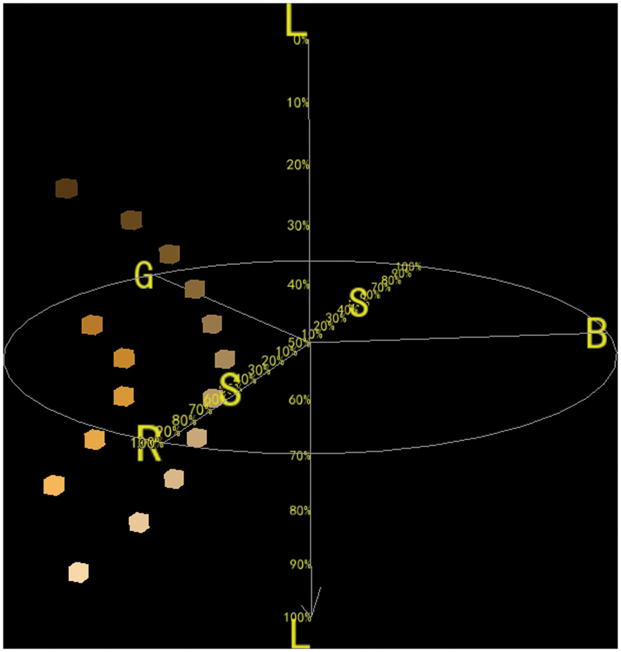
Figure 1: Order chain in HSL color space

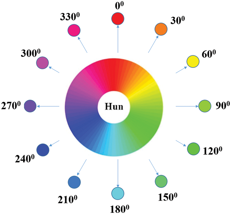
Figure 2: The hun color wheel

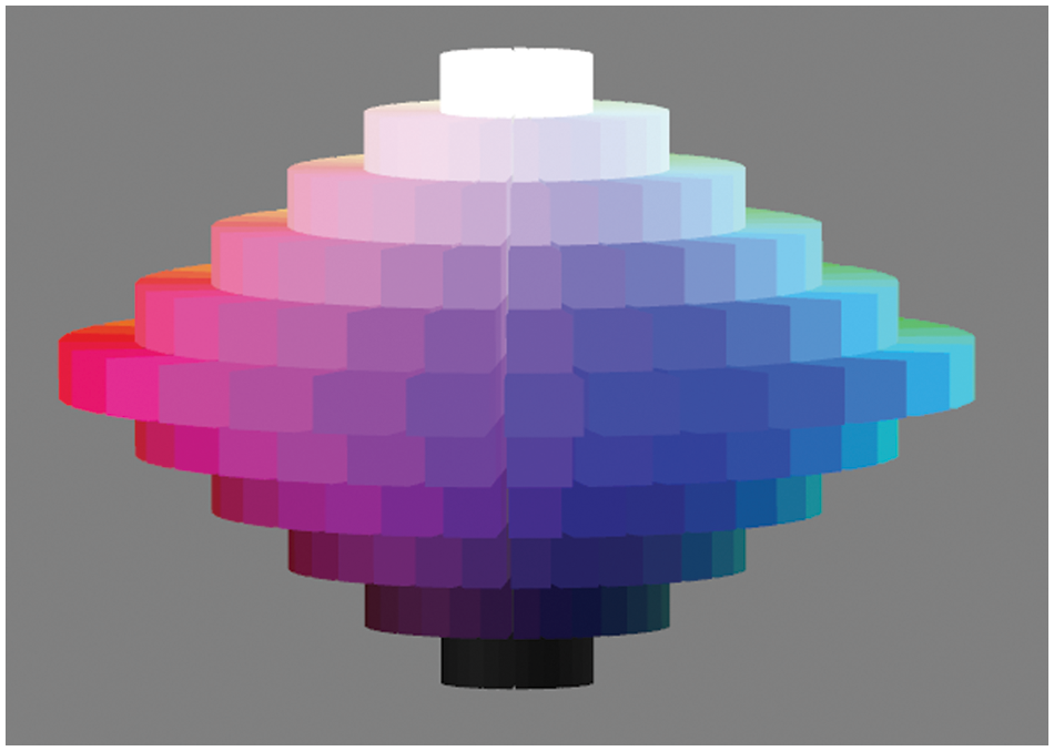
Figure 3: The simulation image of the HSL color solid

In simulation experiments, when the external color factors of simulated plants in the natural environment are disturbed, they form a discrete color law family (the corresponding RGB values are omitted), and the color of the corresponding plants changes accordingly.

By simulating and analyzing the factor α of the color law set of plants when (F,F¯) -interference occurs, according to theorem 3 (Central Limit Theorem) and [25–30], the generation of (H, S, L) law distribution family of HSL space (as shown in Figs. 4, 6), deduce the generated color P-law of HSL, where H is represented using R, G and B, to achieve the intelligent color P-law reasoning simulation based on the natural environment.

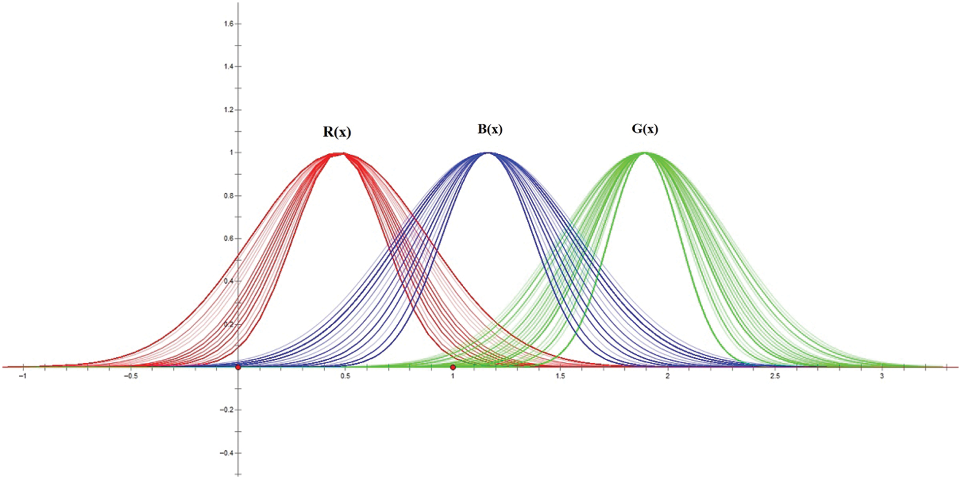
Figure 4: (F,F¯) -interference distribution of the (R, G, B)

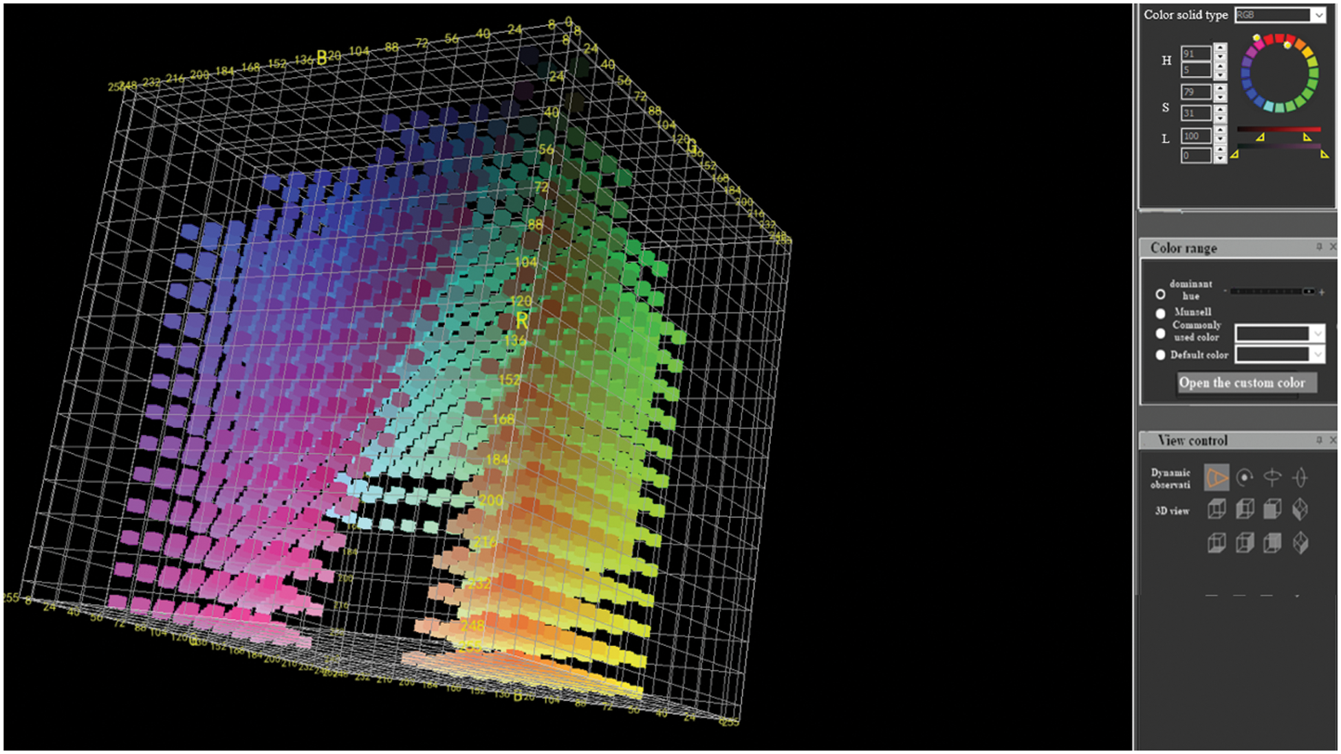
Figure 5: The simulation of the RGB color solid by (F,F¯) -interfered

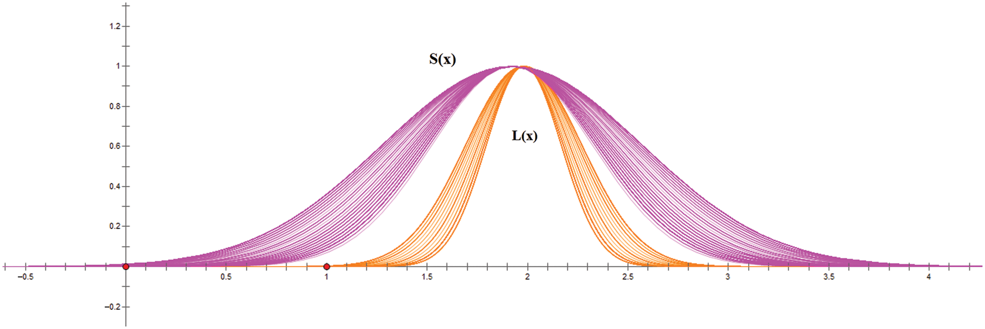
Figure 6: (F,F¯) -interference distribution of the saturation and lightness

The simulation of the RGB color solid by (F,F¯) -interfered is shown in Fig. 5, when 50 ≤ H < 910,31% ≤S≤ 79%, 0 ≤L≤ 100%.

The simulation of the HSL color solid by (F,F¯) -interfered as follows:

When 30 ≤ H < 810, 26% ≤ S ≤ 100%, 26% ≤ L≤ 68% , the simulation of the HSL color solid by (F,F¯) -interfered is shown in Fig. 7.

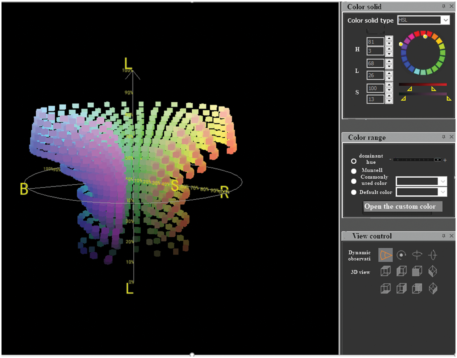
Figure 7: The simulation of the HSL color solid by (F,F¯) -interfered

When 90 ≤ H < 920, 28% ≤ S ≤ 94%, 33% ≤ L ≤ 78%, the simulation of the HSL color solid by (F,F¯) -interfered is shown in Fig. 8.

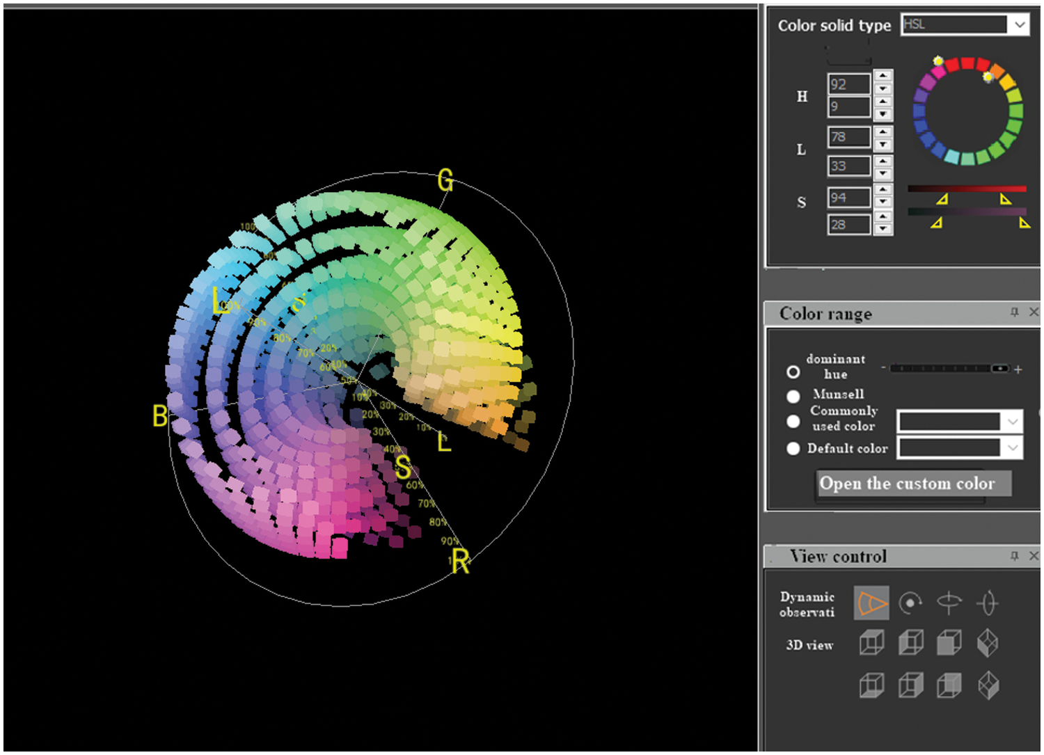
Figure 8: The simulation of the HSL color solid by (F,F¯) -interfered

5  Conclusion

This paper proposes a dynamic color system theory based on the function P-set and presents a color reasoning algorithm for the P-law in a natural environment. The simulation experiment simulates the basic law of color variation when external factors change. The outcome of this paper will be applied in the color simulation of the IoT devices. When the natural conditions in the scene change, the plants will also change autonomously. The proposed algorithm can effectively extract color data, which can significantly reduce the data transmission bandwidth of color sensors in the IoT network.

Since the models and algorithms currently studied only simulate the color factors of plants, there are some points worthy of further study: 1) The time and space complexity of the algorithm can be analyzed; 2) The research and simulation of the color-law relationship between HSL and other standard color stereo, etc. To facilitate the analysis, this paper adopts the calculation method of normal distribution and incorporates the random function into the proposed method to obtain the expected effect, which will be further discussed in the follow-up research.

Acknowledgement: The authors are grateful to the anonymous referees for having carefully read earlier versions of the manuscript. Their valuable suggestions substantially improved the quality of exposition, shape and content of the article.

Funding Statement: This research is supported and funded by the Natural Science Foundation Project of Fujian Provincial Department of science and technology, Grant No.: 2020J01385, Digital Fujian industrial energy big data research institute, Grant No. KB180045, Provincial Key Laboratory of industrial big data analysis and Application, Grant No. KB180029, Sanming City 5G Innovation Laboratory, Grant No.:2020 MK18.

Conflicts of Interest: The authors declare that they have no conflicts of interest to report regarding the present study.

References

 1.  C. T. Poomagal, G. A. Sathish and D. Mehta, “Multi level key exchange and encryption protocol for internet of things (IoT),” Computer Systems Science and Engineering, vol. 35, no. 1, pp. 51–63, 2020. [Google Scholar]

 2.  D. Kim, S. D. Min and S. Kim, “A dpn (delegated proof of node) mechanism for secure data transmission in iot services,” Computers, Materials & Continua, vol. 60, no. 1, pp. 1–14, 2019. [Google Scholar]

 3.  S. K. Kim, M. Koppen, A. K. Bashir and Y. Jin, “Advanced ICT and IOT technologies for the fourth industrial revolution,” Intelligent Automation & Soft Computing, vol. 26, no. 1, pp. 83–85, 2020. [Google Scholar]

 4.  M. Kamiyama and A. Taguchi, “Color conversion formula with saturation correction from HSI color space to RGB color space: Regular section,” IEICE Transactions on Fundamentals of Electronics, Communications and Computer Sciences, vol. 10, no. 7, pp. 1000–1005, 2021. [Google Scholar]

 5.  L. Wang and W. Wang, “Real-time rendering of plant leaves,” SIGGRAPH ‘06 ACM SIGGRAPH 2006 Courses, vol. 1, pp. 712–719, 2006. [Google Scholar]

 6.  Z. M. Amean, T. Low and N. Hancock, “Automatic leaf segmentation and overlapping leaf separation using stereo vision,” Array, vol. 12, no. 12, pp. 100099, 2021. [Google Scholar]

 7.  E. J. Primka and W. K. Smith, “Synchrony in fall leaf drop: Chlorophyll degradation, color change, and abscission layer formation in three temperate deciduous tree species,” American Journal of Botany, vol. 106, no. 3, pp. 377–388, 2019. [Google Scholar]

 8.  Y. Tian, “Advances in appearance modeling and photorealistic rendering of plant leaves,” Journal of Image and Graphics, vol. 17, no. 5,. pp. 613–620, 2012. [Google Scholar]

 9.  F. Xia and S. Huang, “Application research of color design and collocation in image processing,” Computer Systems Science and Engineering, vol. 35, no. 2, pp. 91–98, 2020. [Google Scholar]

10. H. Li, W. Zeng, G. Xiao and H. Wang, “The instance-aware automatic image colorization based on deep convolutional neural network,” Intelligent Automation & Soft Computing, vol. 26, no. 4, pp. 841–846, 2020. [Google Scholar]

11. J. Wang and Y. Zhang, “Median filtering forensics scheme for color images based on quaternion magnitude-phase CNN,” Computers, Materials & Continua, vol. 62, no. 1, pp. 99–112, 2020. [Google Scholar]

12. R. Krishna and S. Kumar, “Color image segmentation using soft rough fuzzy-c-means and local binary pattern,” Intelligent Automation & Soft Computing, vol. 26, no. 2, pp. 281–290, 2020. [Google Scholar]

13. Y. Kang, F. Liu, C. Yang, X. Luo and T. Zhang, “Color image steg analysis based on residuals of channel differences,” Computers, Materials & Continua, vol. 59, no. 1, pp. 315–329, 2019. [Google Scholar]

14. B. Desbenoit, E. Galin and S. Akkouche, “Modeling autumn sceneries,” in Proc. Eurographics, Vienna, Austria, pp. 107–110, 2006. [Google Scholar]

15. F. N. Al-Wesabi, “A smart English text zero-watermarking approach based on third-level order and word mechanism of markov model,” Computers, Materials & Continua, vol. 65, no. 2, pp. 1137–1156, 2020. [Google Scholar]

16. X. Y. Chi, “Simulation of autumn leaves,” Journal of Software, vol. 20, no. 3, pp. 702–712, 2009. [Google Scholar]

17. K. F. Yang, “The visualization of aging process of leaves combined with environmental factors,” M.S. dissertation, Zhejiang University of Technology, China, 2010. [Google Scholar]

18. Y. Tang and D. Y. Wu, “Computational approach to seasonal changes of living leaves,” Computational and Mathematical Methods in Medicine, vol. 2013, pp. 8, 2013. [Google Scholar]

19. H. Zheng and D. Shi, “A Multi-agent system for environmental monitoring using boolean networks and reinforcement learning,” Journal of Cyber Security, vol. 2, no. 2, pp. 85–96, 2020. [Google Scholar]

20. G. B. Bao and H. J. Li, “Large-scale forest rendering: Real-time, realistic, and progressive,” Computers & Graphics, vol. 36, pp. 140–151, 2012. [Google Scholar]

21. K. Q. Shi, “Function P-sets,” International Journal of Machine Learning and Cybernetics, vol. 2, no. 4, pp. 281–288, 2011. [Google Scholar]

22. G. Y. Zhang and E. Z. Li, “Information gene and identification of its information knock-out/knock-in,” An International Journal Advances in Systems Science and Applications, vol. 10, no. 2, pp. 308–315, 2010. [Google Scholar]

23. K. Q. Shi and X. H. Li, “Camouflaged information identification and its applications,” An International Journal Advances in Systems Science and Applications, vol. 10, no. 2, pp. 6, 2010. [Google Scholar]

24. S. L. Huang, W. Wang and D. Y. Geng, “P-Sets and its internal P-memory characteristics,” An International Journal Advances in Systems Science and Applications, vol. 10, no. 2, pp. 216–222, 2010. [Google Scholar]

25. Y. Wang, H. Q. Geng and K. Q. Shi, “The mining of dynamic information based on P-sets and its applications,” An International Journal Advances in Systems Science and Applications, vol. 10, no. 2, pp. 234–240, 2010. [Google Scholar]

26. K. Q. Shi, “P-Sets and its applications,” An International Journal Advances in Systems Science and Applications, vol. 1, no. 2, pp. 209–219, 2009. [Google Scholar]

27. H. K. Lin and Y. Y. Li, “P-Sets and its P-separation theorems,” An International Journal Advances in Systems Science and Applications, vol. 10, no. 2, pp. 209–215, 2010. [Google Scholar]

28. Y. Y. Li, Z. Li and K. Q. Shi, “Generation and recovery of compressed data and redundant data,” in Quantitative Logic and Soft Computing 2010, Berlin, Germany, Springer, pp. 661–671, 2010. [Google Scholar]

29. J. M. Qiu and K. Q. Shi, “F-Rough law and the discovery of rough law,” Journal of Systems Engineering and Electronics, vol. 20, no. 1, pp. 81–89, 2009. [Google Scholar]

30. J. M. Qiu and S. Kaiquan, “F-Interfere law generation and its feature recognition,” Journal of Systems Engineering and Electronics, vol. 20, no. 4, pp. 777–783, 2009. [Google Scholar]

31. D. C. Montgomery, C. Douglas and C. George, “Central limit theorem,” Applied Statistics and Probability for Engineers, vol. 1, pp. 241, 2014. [Google Scholar]