3D Path Optimisation of Unmanned Aerial Vehicles Using Q Learning-Controlled GWO-AOA

1  Introduction

Unmanned Aerial Vehicles (UAVs) are an evolving aerospace technology with immense potential for numerous applications. Even though formerly devoted for defence applications, the range of applications of UAVs have been extended to several commercial and domestic fields. Disaster management and disaster zone mapping [1], construction [2], search and rescue, survey, security, and traffic surveillance [3] are some of the applications in which UAVs have been immensely utilised. The ever increasing usage of UAVs in day-to-day life applications requires the UAVs to autonomously navigate in a real world environment. The accessibility to 3D for traversing and the presence of obstacles make the path planning a perplexing task. The 3D path planning of UAV, aims to create a flyable path in a challenging environment. The path optimisation of UAV enables to detect a safe collision-free flight route.

The path planning of UAVs in 3D environment can be formulated as an optimisation problem, for which the fitness function can be designed and an optimisation technique can be devised to obtain the optimum solution path. The objective of path planning is to construct a collision-free flight route for the UAV from the start to the target position where it is deployed. Along with the collision avoidance, other constraints, such as energy consumption and time required to accomplish the desired path are also considered to frame the objective function. Throughout the literature, metaheuristic algorithms prove to be successful optimisation techniques for several engineering optimisation problems, due to their advantages such as ease of implementation and simplicity [4]. Several proficient metaheuristics have been utilised successfully for path optimisation as well. Furthermore, metaheuristics have been examined to perform better than graph based methods for UAV path planning [5]. The previous literature reveals the employability of metaheuristics for 2D (Two Dimensional) path planning however, for UAVs, it restrict the mobility in any one of the plane [6,7].

For 3D path planning of UAVs, Particle Swarm Optimisation (PSO) and Global Best path competition (GBPSO) have been exhausted in past [8,9]. For military environments containing radar guided Surface-to-Air Missiles (SAM), an Improved Particle Swarm Optimisation (IPSO) algorithm has also been employed [10]. However, PSO struggles with the problem of early convergence and trapping in local minima and therefore, to overcome these limitations, Rauch-Tung-Striebel (RTS) smoother and Metropolis criterion have been extensively incorporated [11]. Recently Double Dynamic Biogeography-Based Learning PSO has also been investigated to improve PSO for UAV path planning [12]. Further, being motivated by the efficacy of Grey Wolf Optimization (GWO), it has been exhaustively utilised with improved and hybrid versions, such as Markov Decision Process based GWO with Level Comparison (GWOLC) [13], Modified Symbiotic Organism Search (MSOS) based GWO [14] and hybrid Golden Eagle Optimiser-GWO [15] for optimal flight route mapping. Considering UAVs as an emerging technology for disaster management, a constrained Differential Evolution (DE) algorithm has been proposed for flight route optimisation [1]. Additionally, Improved Bat Algorithm (IBA) [16] and Glow-worm Swarm Optimisation (GSO) [17] have been employed to estimate the efficient route in static and dynamic environment, respectively. In addition to this, physics inspired optimisers such as Equilibrium Optimiser (EO) [18], Quantum-Entanglement Pigeon-inspired Optimisation (QEPO) [19], Multiverse optimiser (MVO) [20] and Gravitational Search Algorithm (GSA) [21] have been successfully employed for automatic optimal flight path generation in the 3D flight environment. Recently, other physics inspired algorithms have also been introduced such as Archimedes Optimisation Algorithm (AOA) [22], Flow Direction Algorithm (FDA) [23], Artificial Electric Field Algorithm (AEFA) [24], etc. However, the capabilities of these developed algorithms for optimal path planning have been seldom examined. Apart from metaheuristics, other Artificial Intelligent (AI) techniques such as Heuristic search, Artificial Neural Networks, Local search techniques have been studied extensively for UAV path planning [25].

Moreover, with the advent of Machine Learning (ML), enormous work has been extensively reported to elevate the optimisation capabilities of metaheuristics. In this sequence, Reinforcement Learning (RL) has been commonly utilised to control the exploration and exploitation behaviours [26]. The efficacy of RL based metaheuristic for UAV flight route planning has been validated to achieve better flying path and convergence speed [27]. Furthermore, as per No Free Lunch (NFL) [28] theorem, an optimisation algorithm promising good performance in terms of accuracy and convergence speed on one set of problems does not ensure similar performance on other set of problems. This provides a possibility to develop a new and advance optimization algorithms for UAV path planning.

Therefore, the present work investigates the possibilities to develop a novel metaheuristic by employing AOA and GWO. Further, the RL based algorithm selection mechanism has been developed in order to reach the new horizons with proposed metaheuristics. In AOA, the capability to optimize any real time optimization problem has been controlled by transfer operator that maintains the global-local search balance. The transfer operator assures that the first 30% iterations are exploration, by updating the individual positions based on the position of a randomly selected individual. During the next phase, the exploitation, the positions of the individuals are updated utilising the position of the best individual. However, the low convergence speeds of AOA is the consequence of absence of exploitation during the first one-third iterations. Additionally, the previous literature comprehensively employed the use of GWO for UAVs path planning because of its higher convergence speed and capability to generate optimum path with obstacle [29,30]. The GWO estimates three best individuals, alpha, beta, and delta wolves and the positions of all the individuals are updated based on these best individuals. This ensures good exploitation capacity for the GWO algorithm however, it suffers by the premature convergence and stagnation at local minima [31].

To effectively address the above mentioned issues, the Q learning controlled GWO-AOA (QGA) has been proposed in the present work. The exploitation capabilities of GWO and the exploration abilities of AOA have been combined in the introduced algorithm. For maintaining the balance between global and local search, ϵ greedy Q learning has been employed [32]. The Q learning states and actions are labelled as AOA and GWO. The Q learning agent selects between GWO and AOA according to the Q table values to achieve maximum reward. The incorporation of Q agent for regulating the exploration and exploitation balance will provide higher convergence rates and prevents trapping in the local optimal solutions.

The performance of the developed QGA has been validated against 22 popular benchmark functions and then, employed to estimate the optimum path for UAVs. For this purpose, the results obtained for the benchmark functions have been compared with GWO, AOA, RL based GWO (RLGWO) [27], Enhanced AOA (EAOA) [33], and PSO [34]. Further, the popular statistical test such as Friedman test and Wilcoxon rank-sum test have also been executed on the benchmark results to endorse the efficacy of the compared metaheuristics. For path planning also, the developed QGA has been exhaustively compared with aforementioned metaheuristics under complex 3D environment. Summarising the main contribution of the present investigation are:

•   Development of Q-controlled GWO-AOA (QGA) to enhance the exploration-exploitation balance.

•   Development of algorithm selection mechanism to efficiently select the employed metaheuristics based on Q-State parameters.

•   Exhaustive validation of developed QGA against other metaheuristics for various benchmark functions based on statistical tests.

•   Examining the employability of QGA for real-time path-planning optimization problem of UAV in 3D environment.

The rest of the paper is organised as follows. Section 2 includes the brief description about Q learning, GWO, and AOA. The detailed description of the proposed QGA is presented in Section 3. The path planning problem statement is formulated in Section 4. The performance analysis of QGA over benchmark functions and the effectiveness of proposed algorithm for path planning in 3D flying field is presented in Section 5. Lastly, Section 6 concludes the work with discussions on future research.

2  Background

2.1 Q Learning

RL comprises four sub-elements, namely, policy, reward signal, a value function, and a model of the environment. RL depends on the interactivity between the learning agent and its environment. Reward signal is the feedback from the environment to the RL agent which quantifies this interactivity. Q learning is an off policy Temporal Difference (TD) method. Q indicates the action-value function. One of the main components of Q learning is the Q table. The reward is the reinforcement signal which guides the learning agent during the process. The main objective of the learning agent is to maximise the reward signal. The Q value is dependent on the reward signal. During each operation, the Q table is updated based on the Eq. (1). For each state-action pair there will be a corresponding Q table value ( Q(Sitr,Aitr) ). Each Q table update depends on the reward signal ( Reward ) from the environment. The goal of maximizing the reward at the end of the operations is ensured by performing an action with the highest Q value.

Qitr+1(Sitr,Aitr)=Q(Sitr,Aitr)+μ(Rewarditr+1+γmaxAQ(Sitr+1,Aitr)−Q(Sitr,Aitr)) (1)

where, S is the state, A is the action, itr is the current iteration, μ indicates the learning rate, and γ denotes the discount factor.

2.2 Archimedes Optimisation Algorithm (AOA)

The Archimedes Optimisation Algorithm (AOA) is based on Archimedes’ principle that defines the relation between buoyant forces or upthrust and the weight of the displaced fluid. According to Archimedes’ principle, if a body is completely or partially immersed in a liquid, the net upward force, also known as the buoyant force acting on the body will be equal to the weight of the liquid displaced by the body. If the weight of the displaced liquid is greater than the upward force, the body will be completely immersed in the liquid whereas, if the weight of the body is equal to the weight of the displaced liquid, the body will be floating in the liquid. The initial population of AOA consists of various bodies with different densities and volumes. Each of these bodies will try to achieve an equilibrium state with neutral buoyancy. This can be mathematically represented by Eq. (2), which is further expanded to Eq. (3)

Fliq=Fb (2)

ρliqVliqacnliq=ρbVbacnb (3)

where, ρliq , Vliq , and acnliq are the density, volume and acceleration of the liquid, respectively. Similarly, ρb , Vb , and acnb are the density, volume and acceleration of the object floating in the liquid, respectively.

To obtain the acceleration of the body, Eq. (3) is rearranged as shown in Eq. (4)

acnb=ρliqVliqacnliqρbVb (4)

If other forces such as collision with other bodies are affecting the body under consideration, Eqs. (2)–(3) are modified as Eqs. (5)–(6) respectively.

Wliq−Web=Fb (5)

ρliqVliqacnliq−ρebVebacneb=ρbVbacnb (6)

where, ρeb , Veb , and acneb denotes the density, volume, and acceleration of the external object, Wliq is the weight of the liquid displaced and Web is the weight of the external object.

The initial position ( Pbi ) and acceleration ( acnbi ) of the i th body immersed in the liquid are generated using Eqs. (7)–(8). The density and volume of each body is initialised randomly in the range [0, 1].

Pbi=lbb+r1(ubb−lbb) (7)

acnbi=lbb+r2(ubb−lbb) (8)

where, r1 and r2 indicates random numbers in the range [0, 1], lbb and ubb are the lower bounds and upper bounds of the search space, respectively.

The density factor and transfer operator helps in maintaining exploration-exploitation balance in AOA. During first 30% of the iterations, AOA is in global search followed by the local search. The exploration and exploitation phases are defined using transfer operator ( TR ) defined by Eq. (9). Density factor ( df ) represents the exploration to exploitation shift and is calculated by Eq. (10).

TR=exp(itr−MaxMax) (9)

df=exp(itr−MaxMax)−(itrMax) (10)

where, itr and Max depicts the current iteration and maximum number of iterations, respectively.

During each iteration the density ( ρbi ) and volume ( Vbi ) of each body are updated using Eqs. (11)–(12).

ρbi(itr+1)=ρbi(itr)+r3(ρalpha−ρbi(itr)) (11)

Vbi(itr+1)=Vbi(itr)+r4(Valpha−Vbi(itr)) (12)

where, r3 and r4 corresponds to the random numbers [0, 1], ρalpha and Valpha represents the best density and volume of the body obtained from the previous iteration, respectively.

Further, if TR≤0.5 , exploration is performed and, the acceleration and position are updated using the previously selected random body, respectively. This acceleration update mechanism is represented by Eq. (13) where, ρbr , Vbr and acnbr denotes the density, volume and acceleration of the randomly selected body respectively.

acnbi(it+1)=ρbr+Vbracnbrρbi(itr+1)Vbi(itr+1) (13)

Then, the acceleration, acnbi is normalised using Eq. (14), where, u and l are constants.

norm_acnbi(itr+1)=u×acnbi(itr+1)−min(acn)max(acn)−min(acn)+l (14)

The position of i th individual during the exploration stage is updated using Eq. (15).

Pbi(itr+1)=Pbi(itr)+c1×r5×norm_acnbi(itr+1)×df×(Pbr−Pbi(itr)) (15)

where, c1 is a constant, r5 is a random number, and Pbr is the position of the selected random object.

Moreover, if TR > 0.5, the algorithm will perform local search (exploitation). The acceleration is updated using the Eq. (16) and then normalised by employing Eq. (14).

acnbi(itr+1)=ρalpha+Valphaacnalphaρbi(itr+1)Vbi(itr+1) (16)

where, ρalpha , Valpha , and acnalpha indicates the density, volume, and acceleration of the best body obtained so far, respectively.

Afterwards, if Palpha is the position of the body with best fitness function then, the position of the i th body is updated by Eq. (17) considering c2 and r6 as constant and random number, respectively.

Pbi(itr+1)=Palpha(itr)+Flag×c2×r6×norm_acnoi(itr+1)×df×(TF×Palpha−Pbi(itr)) (17)

Additionally, based upon the constant ( c3 and c4 ) and random value ( r7 ), TF and Flag are also regularly estimated by Eqs. (18)–(20).

TF=c3×TR (18)

Flag={+1,ifF≤0.5−1,otherwise (19)

F=2×r7−c4 (20)

2.3 Grey Wolf Optimisation (GWO)

The Grey Wolf Optimisation (GWO) is inspired from the hunting behaviours and social hierarchy of grey wolf packs. Grey wolves live in groups called packs and maintain a strict social hierarchy among the group. The topmost leader of the group is called the α wolf, followed by leader groups, the β , and the δ wolves, and the rest of the pack is called as the ω wolves. The candidate solutions (wolf population) is updated based on the leader groups which represent the best, the second best, and the third best solutions, respectively using Eqs. (21)–(28).

Pbi(itr+1)=(P1+P2+P3)/3 (21)

P1=Palpha(itr)−A1Dalpha (22)

P2=Pbeta(itr)−A2Dbeta (23)

P3=Pdelta(itr)−A3Ddelta (24)

Dα=|C1Palpha(itr)−Poi(itr)| (25)

Dβ=|C2Pbeta(itr)−Poi(itr)| (26)

Dδ=|C3Pdelta(itr)−Poi(itr)| (27)

Ck=2rck

Ak=2at.rtk−at (28)

where, at is linearly decreased from 2 to 0 during each iteration, rck is a random number which gives Ck , k=1,2,3 , rtk is another random number used to calculate the parameter Ak , Pbi(itr) is the position of i th candidate solution at the current iteration itr , Pbi(itr+1) is the updated position. Pbi is given by the mean of P1 , P2 , and P3 , which depends on the positions of the leader group, Palpha , Pbeta , and Pdelta , respectively.

3  The Q Learning-Controlled GWO-AOA

GWO and AOA are both population based algorithms. In the case of AOA, the exploration and exploitation behaviour is selected by TR which leads to slow convergence rate. In GWO, extremely efficient exploitation capabilities are witnessed because of the dependence on the leader group only. However, this also reduces the population diversity which lead to premature convergence and premature local minima. Therefore, the GWO and AOA are combined to obtain more efficient global-local capabilities. But, selecting a particular optimization algorithm at different stages is very challenging task and therefore, the artificially intelligent, Q learning is employed. Additionally, premature convergence and stagnation at local optima can also be avoided since, the Q agent maintains the balance between exploration and exploitation. The Q agent makes selection based on the Q table values, such that it enables to increase the reward as the iterations progress. The reward is assigned to the agent when the performance is improved. The accumulated performance along with reward decides the change of state or action selection.

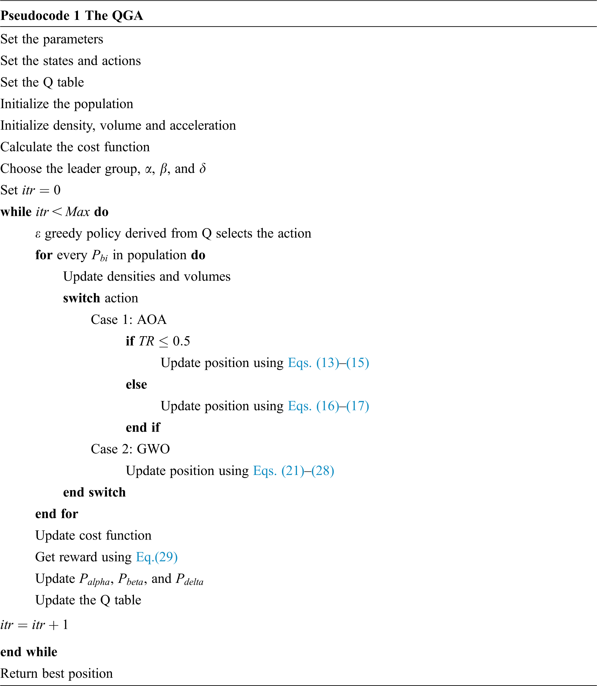
The Q learning is a value based RL technique where, Q denotes the action-value function. In this work, two actions and states are defined, AOA and GWO. The Q table contains the Q values for each state-action pair. The training agent and the environment are represented by the individuals of the population and the search space, respectively. During each operation, the Q table is updated using Eq. (1) and the exploration-exploitation balance is maintained using ϵ greedy policy. As per policy, exploration operation is performed with a probability, 1−ϵ , and exploitation with a probability, ϵ . The exploitation operation forces the Q agent to attain maximum reward by choosing the current best selection, whereas exploration indicates a random selection. The flowchart for the algorithm is illustrated in Fig. 1.

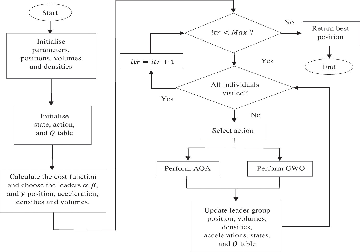
Figure 1: Flowchart for QGA

The agent decides the next action based on the Q table values, which are further depending on the reward signal. By selecting the action with the maximum Q value during the exploitation operation, the agent maximizes its reward. When an operation results in a better cost function value, a positive reward is assigned, otherwise, the Q agent is penalised by a negative reward. If Reward indicate the reward signal achieved by the agent from the environment then the reward assignment is represented by Eq. (29).

Reward={+1,ifcostfunctionisimproved−1,otherwise (29)

4  The Path Planning

4.1 Problem Formulation and Cost Function

The present work attempts to formulate the NP Hard problem such as UAV path planning in 3D environment as an optimisation problem and metaheuristics is found as the most effective approach to solve such problems. The prime objective of path planning for UAV is to find an optimal flyable path from source to destination without collisions in minimum time and energy. To fulfill these requirements, the cost function is formulated based on [14] and [27]. Then, an initial population of candidate paths is generated and by employing an optimisation algorithm, the feasible path is achieved as per the designed cost function. The shortest path between the start and target position have M waypoints, which are initialised with coordinates, (xml,yml,zml) , where ml=0,1,2,…,M then, the population individuals for optimisation with 2M dimension is initialised as shown in Eq. (30).

Pi=[yi1,yi2,…yiM,zi1,zi2,…ziM] (30)

where, yik and zik are the y and z coordinates of the k th waypoint of the i th individual. Initially, the population individuals, Pi , are generated randomly and then, the QGA is employed to optimise the cost function during each iteration.

The cost function to be minimised for the optimal flight trajectory from start to target position is formulated considering the collisions with the obstacles in the environment, energy consumption, and travel time. The collision cost, Fcollision is defined to indicate the collision with any obstacles in the flying environment. The energy consumption will be low for the path with shortest length. The shortest possible collision-free path will also have minimum travel time. Therefore, the cost function, Fcost , is computed as the weighted sum of the collision cost, energy cost, and the deviation cost. Hence, Fcost is represented as shown in Eq. (31),

Fcost=p1Fenergy+p2Fcollision+p3Fdeviation (31)

Since the length of the path is directly proportional to the energy consumption, the energy cost ( Fenergy ) is estimated as the length of the path. When the generated flight path passes through the obstacles present in the environment, a collision cost is evaluated. The flight path with length, l, is divided into M, number of waypoints from start to target positions. For calculating the collision cost, each path segment is again divided into 5 equidistant points, and each of these path segments is examined whether, they are passing through the obstacle or not. If the path segment of length, lm is colliding with an obstacle j as shown in Fig. 2 then, Fcollision is calculated by Eqs. (32)–(33), otherwise, fcollision,lm is assigned as zero (Eq. (33)). Here, s0.25,jm is the length from the centre of the obstacle to the second equidistant point on the path segment, rj is the base radius of the obstacle and N is the maximum number of obstacles.

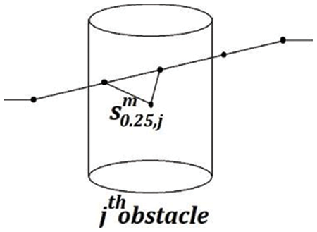
Figure 2: Calculating the collision cost

Fcollision=∫0l⁡fcollisiondl (32)

fcollision,lm=lm5∑j=1N15(|s0,jm−rj|+|s0.25,jm−rj|+|s0.5,jm−rj|+|s0.75,jm−rj|+|s1,jm−rj|) (33)

The deviation cost, Fdeviation , is calculated using Eqs. (34)–(35)

Fdeviation=∫0l⁡fdeviation (34)

fdeviation=(ym−yml)2+(zm−zml)2 (35)

where, ym and zm are the y and z coordinates respectively of the m th waypoint of obtained path, yml and zml are the y and z coordinates respectively corresponding to the m th waypoint on the shortest path between the start and the target position. Further, to generate the flyable path for UAVs, the obtained path is smoothen by employing cubic spline curves [35,36].

4.2 Simulation Environment

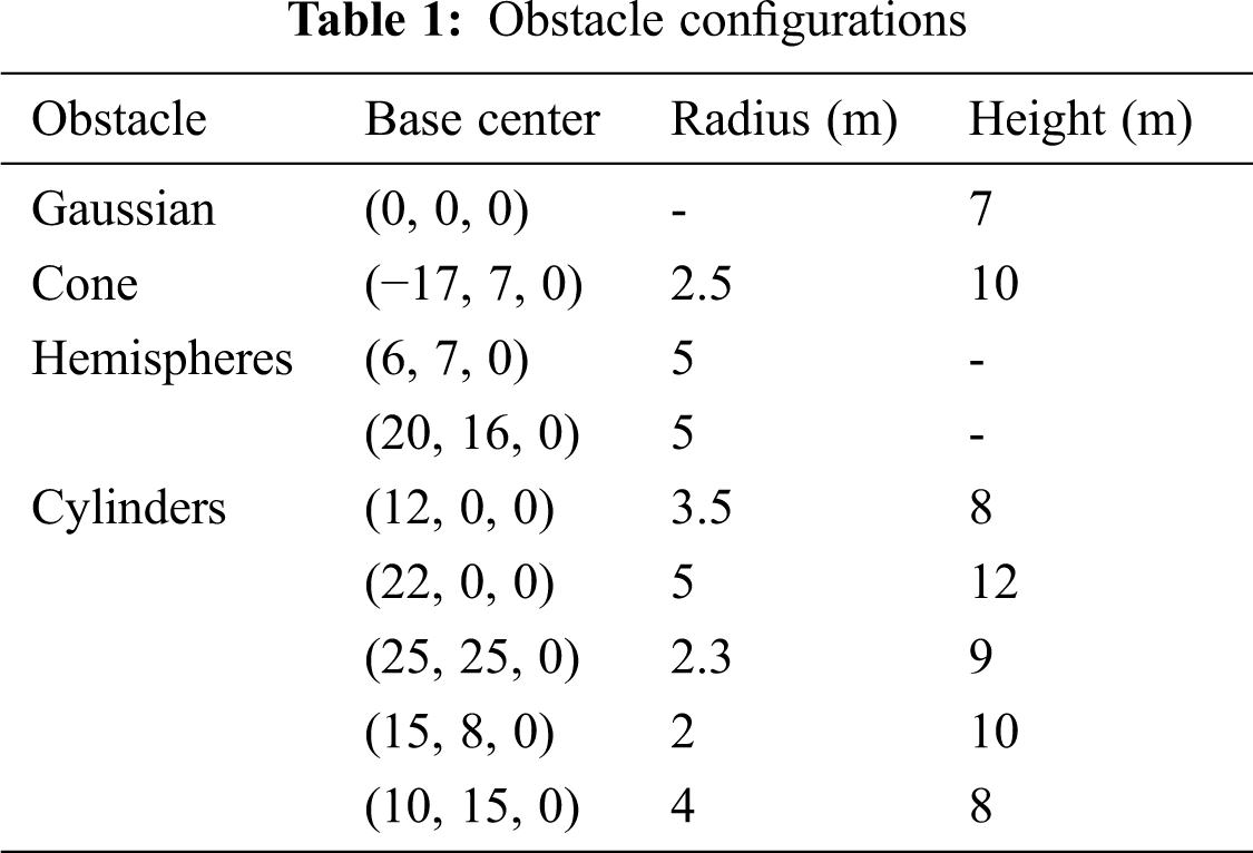
A real world 3D UAV flight environment will contain several threats. Hence, in order to prove the efficiency of the developed algorithm, a simulation environment that resembles the real world civilian environment is required. Therefore, for simulating the results a 3D flight environment consisting of different kinds of obstacles is created. The 3D environment constitutes a Gaussian obstacle, cone, hemispheres, and cylinders of various sizes. The configurations of the simulated obstacles are presented in Tab. 1. The proposed algorithm is utilised to minimise the cost function to obtain an optimal flight path. Finally, all the simulation work are accomplished on the MATLAB 2019a programming platform installed in the Windows-10 operating system with an AMD Ryzen 5 (2.10 GHz) processor and 8GB RAM.

5  Results and Discussions

5.1 Benchmark Function Analysis

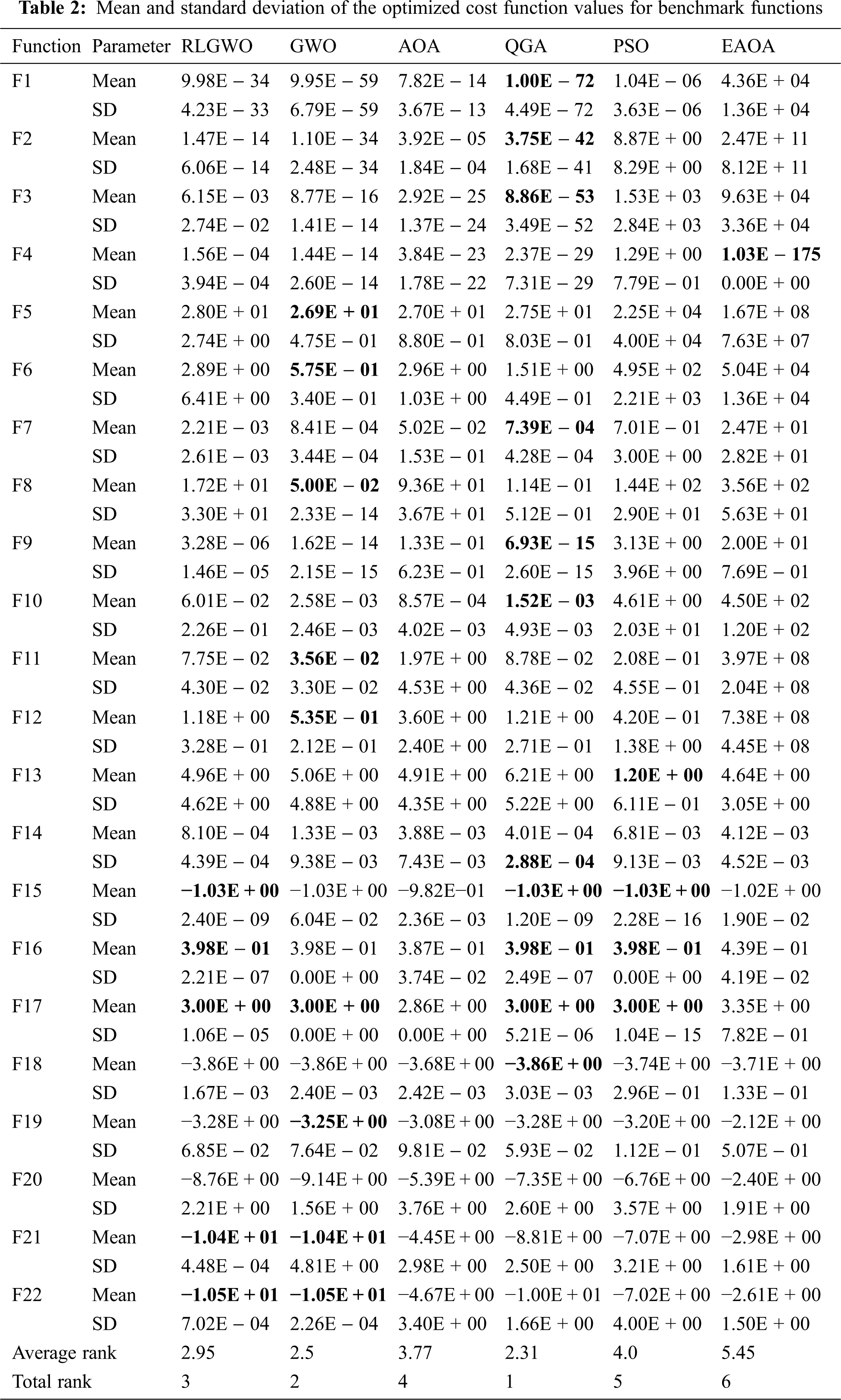
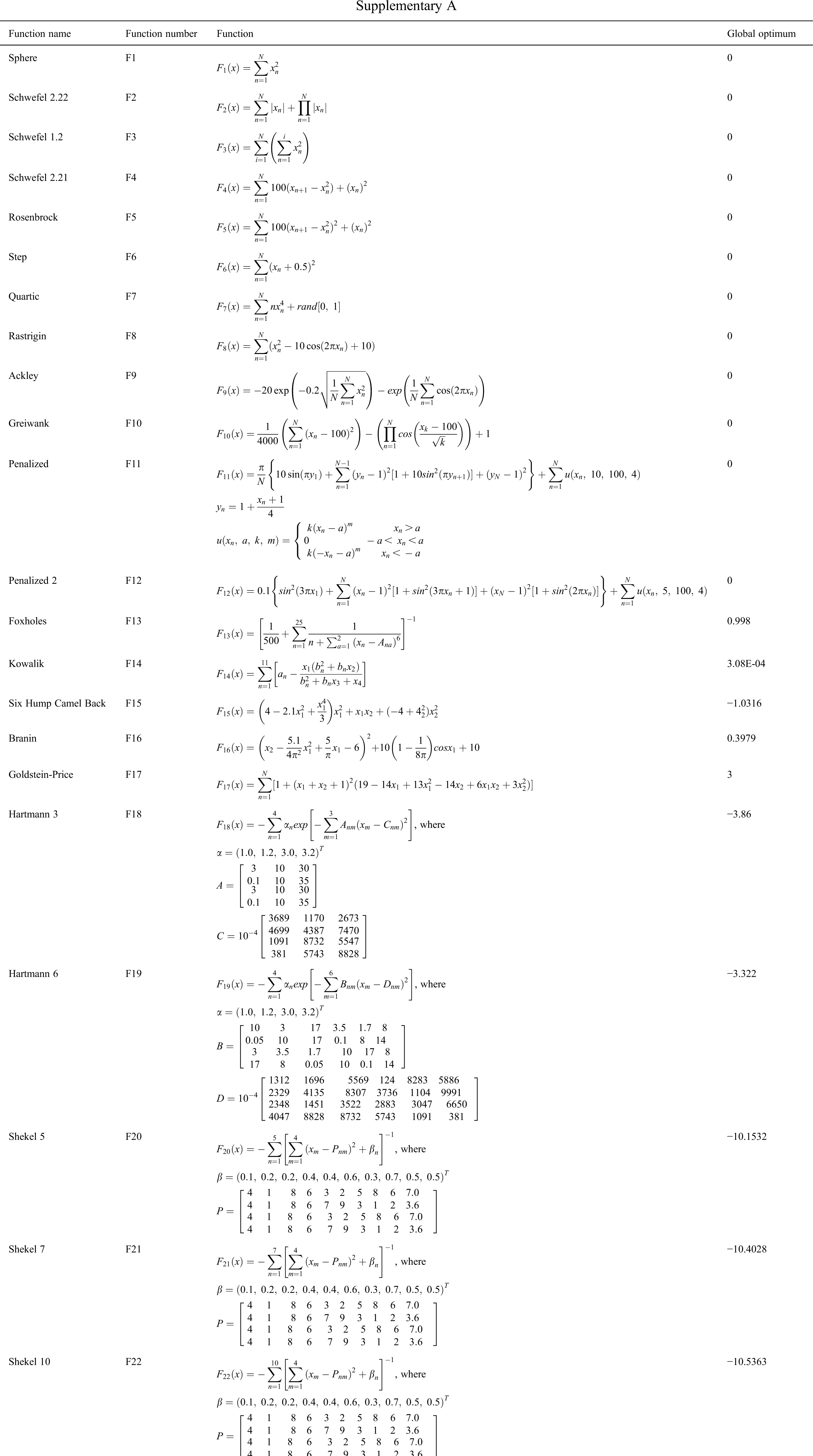
The performance of the developed QGA is evaluated on 22 benchmark functions as mentioned in Supplementary A. The obtained simulated results are compared with GWO, AOA, RLGWO, EAOA, and PSO. The results are analysed for 20 runs, with the maximum number of iterations limited to 1000. The population size is chosen as 30 for all the algorithms for fair comparison. Further, the statistical performance parameters such as Mean and Standard Deviation are computed using the obtained simulated results from 20 runs and tabulated in Tab. 2. Moreover, for the estimation of the rank and overall performance validation, Friedman test is performed and average rank based on the test is also rendered in Tab. 2. The obtained results reveals that QGA is able to provide optimal or near optimal mean values compared with GWO, AOA, PSO, EAOA, and RLGWO for 11 benchmark functions. GWO is resulting in optimal average solutions for 9 benchmark functions, whereas, RLGWO provided optimal average results for 5 only. Therefore, QGA outperforms others by minimum margin of approximately 22%. This is also validated by the Friedman test which estimates the average rank of QGA as 2.31 that is lower than 7.60% by its nearest counterpart. Conclusively, the QGA is ranked 1 as per the Friedman test among the 6 algorithms under consideration.

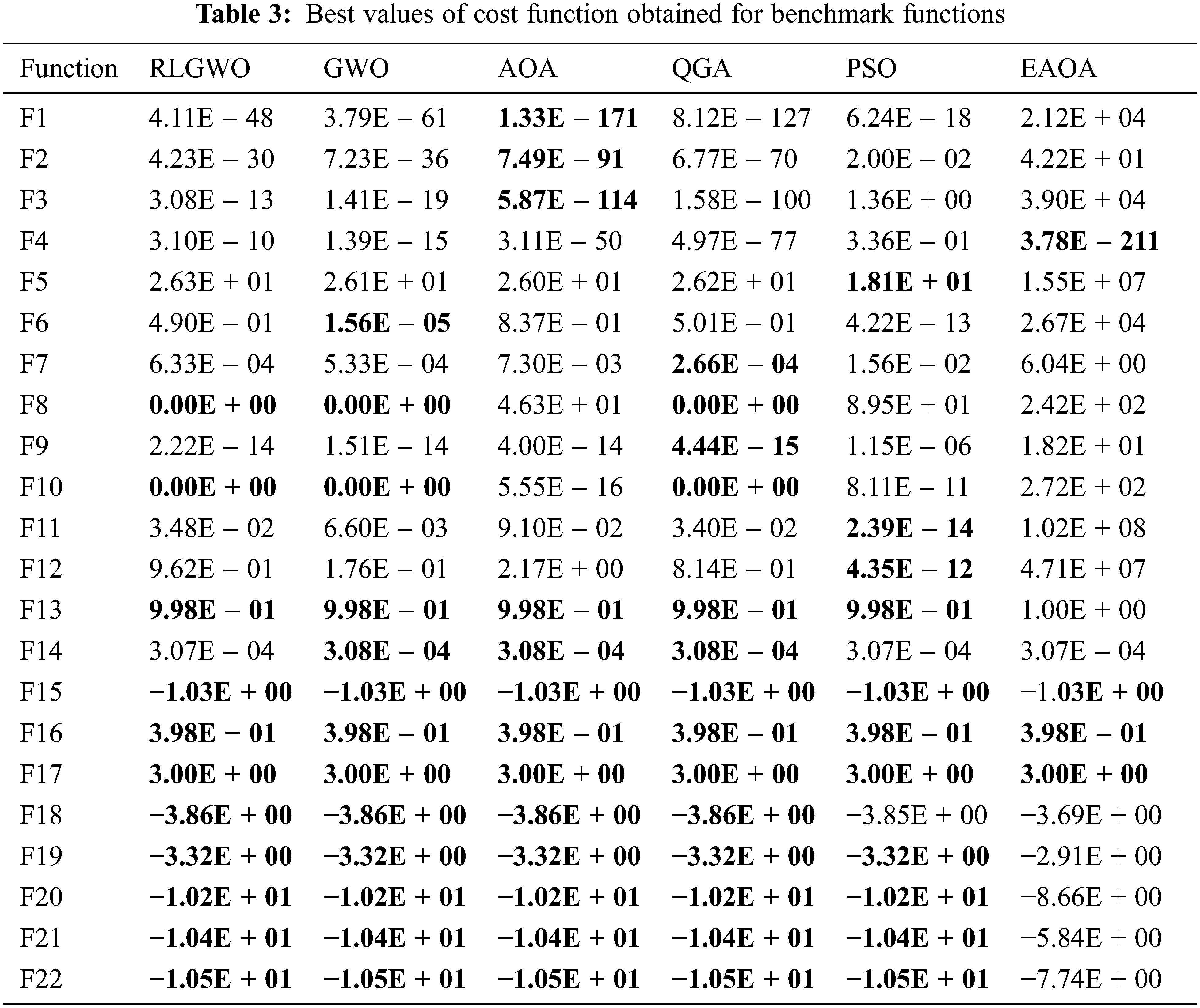
Further, the optimum value for each benchmark are computed against the simulated runs and tabulated in Tab. 3 which is also used to select the convergence curves of the respective benchmark. The QGA is able to provide optimal values for 14 functions. Hence, for 63.60% of the benchmark, the QGA provides an optimal or near optimal solutions for the considered 22 benchmark functions; whereas, GWO, AOA, RLGWO, PSO and EAOA achieved the optimum values for 59%, 59%, 50%, 50% and 18.18% functions, respectively. Therefore, the QGA dominates all the other comparison algorithm by a significant margin of 4.6%, 4.6%, 13.07%, 13.60% and 45.42%, respectively.

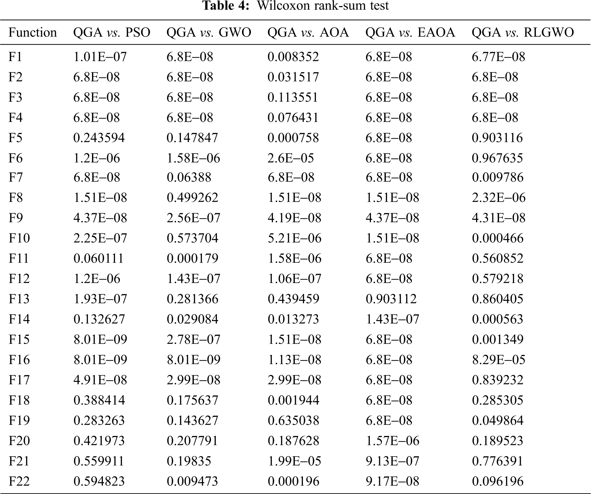
The P values evaluated for Wilcoxon rank-sum test are denoted in Tab. 4. The P value less than 0.05 indicates the statistical significance of QGA compared to the other algorithms. When compared with PSO, the QGA is achieving statistically significant results for 14 functions. For 12 benchmark functions, the QGA provides statistically significant results when compared with GWO. Except for the benchmark functions, F3, F4, F13, F19, and F20, the cost function values achieved by QGA is statistically significant than AOA. While comparing with EAOA, the QGA attains statistically significant cost function values for all the considered functions except the benchmark function F13. The comparison with RLGWO shows that for 12 functions, the QGA is achieving statistically significant results. Therefore, it is perceived that according to Wilcoxon rank-sum test also, the QGA exceedingly dominates all the other employed algorithms.

Finally, the performance of all the employed algorithms is also compared based on convergence plots and sample of these are presented in Fig. 3. It is very obvious from these plots, the QGA shows the faster convergence compared to others and therefore, the adaptive algorithm selection mechanism based on Q learning enables faster convergence without compromising accuracy.

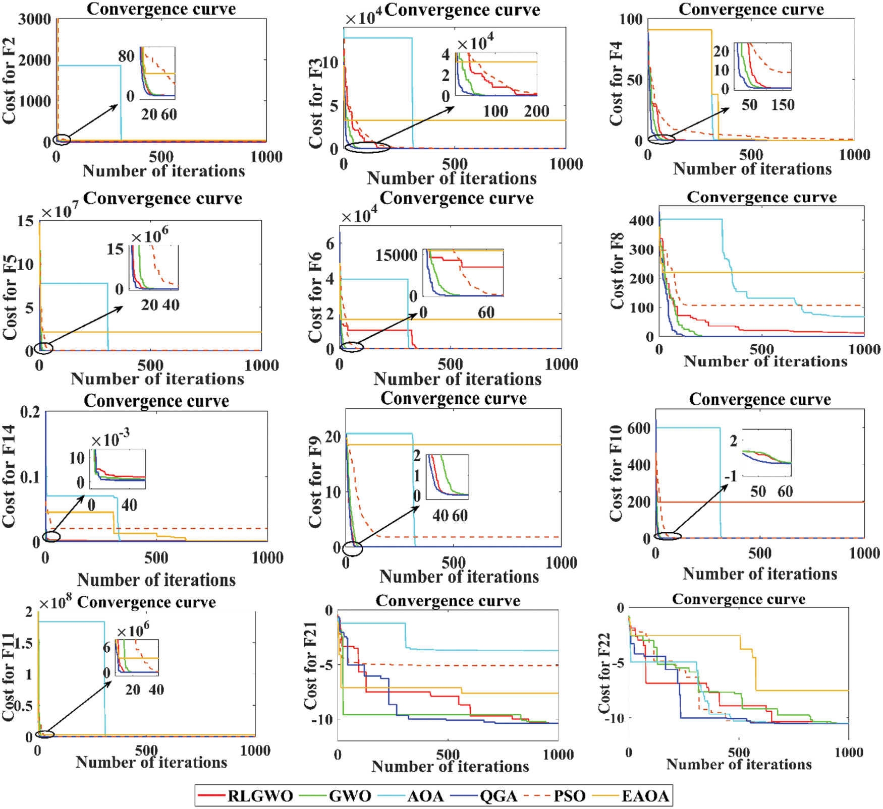
Figure 3: Convergence curves for selected benchmark functions

5.2 Path Planning Results

The developed algorithm is employed to generate 3D flight path in the simulated environment. The maximum number of iterations utilised is 1500, with a population size of 50, for all the algorithms. The results are compared with GWO, AOA, EAOA, RLGWO, and PSO. The Fig. 4 provides the top view of the simulated environment and the generated paths. The 3D view of the created paths in the flight environment is depicted in Fig. 5. The simulated results confirmed that QGA is providing the optimal flight path. From these figures, it is witnessed that only QGA, RLGWO and AOA are able to avoid the collision while estimating the optimum path however, both RLGWO and AOA are consuming higher fuel. Therefore, only QGA successfully estimates the optimum flyable path with all the considered constraints. Not only PSO, EAOA and GWO fails to avoid collision but also the length of the traced path is higher compared to the path generated by QGA.

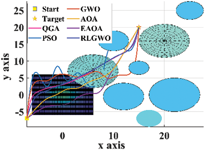
Figure 4: 2D top view of the paths

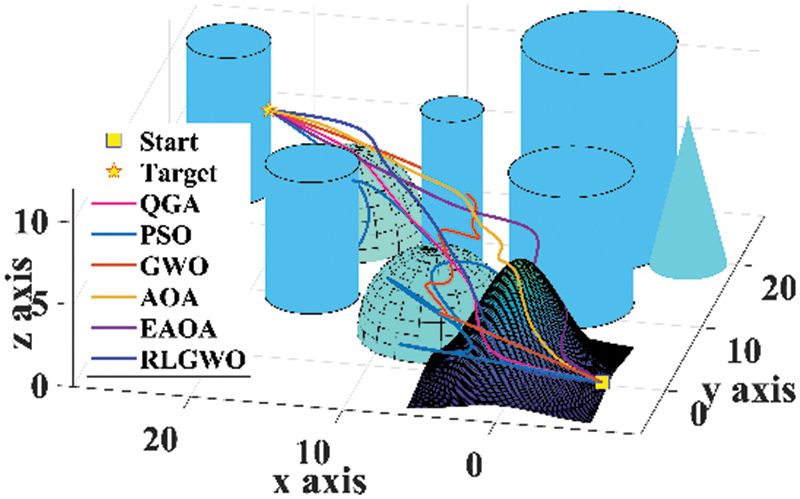
Figure 5: 3D view of the paths

By comprehensive analysis of the convergence curves shown in Fig. 6, it is quite evident that though QGA is converging slower as compared to GWO, EAOA, and PSO but, the QGA is able to achieve collision free optimal flight path. Also, the final optimized objective function values achieved by QGA is significantly lower than that of EAOA, PSO, and GWO.

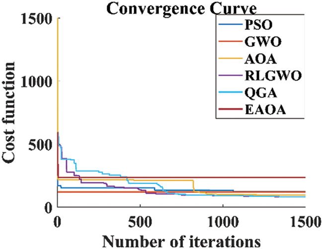
Figure 6: Convergence curve for path planning

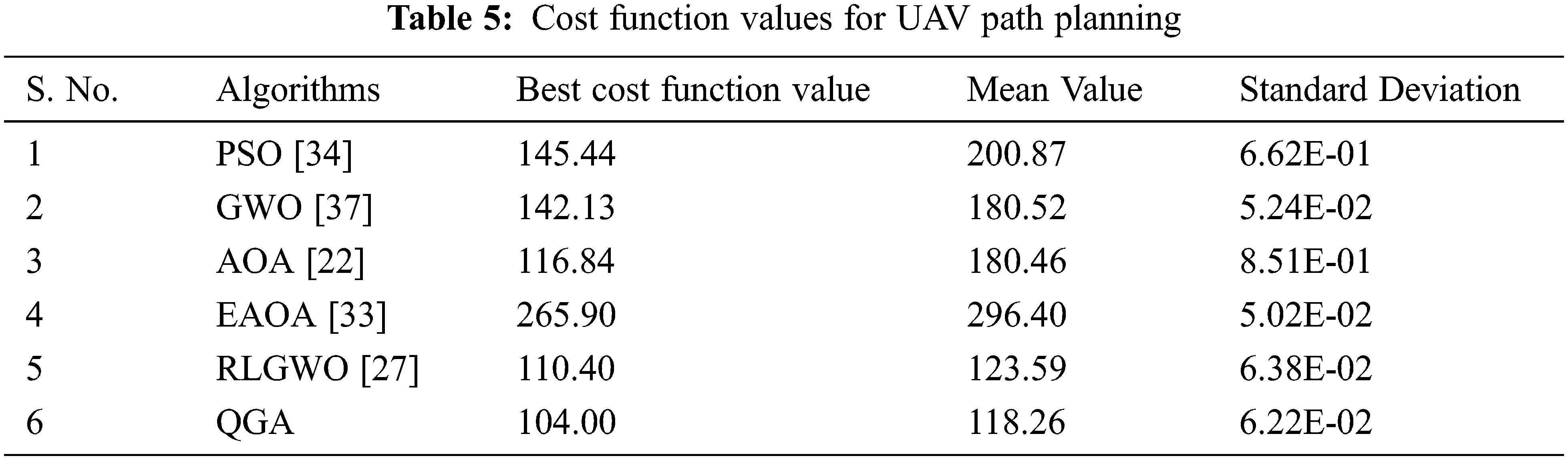
Tab. 5 demonstrate the ability to generate the optimal flyable path for UAVs by the developed QGA with others based on the statistical means. All the employed algorithms are used to estimate the path for 20 runs. The obtained results reveals that the developed QGA achieved the optimum cost value function which is approximately 28.50%, 26.83%, 11.00%, 60.90% and 5.80% lesser than PSO, GWO, AOA, EAOA and RLGWO, respectively. Similarly, Mean value and Standard Deviations are estimated as 4.31% and 2.51% lesser than its nearest competitor (RLGWO).

6  Conclusions

In the present work, a novel Q learning control GWO-AOA (QGA) has been proposed and validated on 22 different benchmark functions based on convergence curves, Freidman test, and Wilcoxon rank-sum test. Additionally, the employability of QGA has been investigated for path planning of UAVs in three dimensional environment. The experimental results reveals that the adaptive algorithm selection mechanism based on Q learning enables QGA to achieve better exploration-exploitation capabilities because of which it dominates all the compared algorithms for both benchmark evaluations and path planning of UAVs. Moreover, the cubic-spline curves has been utilized to smooth the generated flight path for various adopted algorithms. The employability and superiority of the compared algorithms has been comprehensively endorsed on the basis various statistical results and convergence curve analysis. Though, the developed QGA achieved optimum cost for both benchmark and path planning of UAVs, it is not the fastest one which open the window for the future research.

Acknowledgement: The authors extend their appreciation to Princess Nourah bint Abdulrahman University Researchers Supporting Project number (PNURSP2022R66), Princess Nourah bint Abdulrahman University, Riyadh, Saudi Arabia.

Funding Statement: This research was funded by Princess Nourah bint Abdulrahman University Researchers Supporting Project number (PNURSP2022R66), Princess Nourah bint Abdulrahman University, Riyadh, Saudi Arabia.

Conflicts of Interest: The authors declare that they have no conflicts of interest to report regarding the present study.

References

 1.  X. Yu, C. Li and J. F. Zhou, “A constrained differential evolution algorithm to solve UAV path planning in disaster scenarios,” Knowledge-Based Systems, vol. 204, pp. 106209, 2020. [Google Scholar]

 2.  M. C. Tatum and J. Liu, “Unmanned aircraft system applications in construction,” Procedia Engineering, vol. 196, no. June, pp. 167–175, 2017. [Google Scholar]

 3.  H. Gupta and O. P. Verma, “Monitoring and surveillance of urban road traffic using low altitude drone images: A deep learning approach,” Multimedia Tools and Applications, vol. 81, no. 14, pp. 19683–19703, 2021. [Google Scholar]

 4.  S. Mirjalili and A. Lewis, “The whale optimization algorithm,” Advances in Engineering Software, vol. 95, pp. 51–67, 2016. [Google Scholar]

 5.  S. Ghambari, J. Lepagnot, L. Jourdan and L. Idoumghar, “A comparative study of meta-heuristic algorithms for solving UAV path planning,” in Proc. of the 2018 IEEE Symposium Series on Computational Intelligence, SSCI 2018, Banglore, India, pp. 174–181, 2019. [Google Scholar]

 6.  M. Cakir, “2D path planning of UAVs with genetic algorithm in a constrained environment,” in 6th Int. Conf. on Modeling, Simulation, and Applied Optimization 2015, ICMSAO, Istanbul, Turkey, 2015. [Google Scholar]

 7.  T. Turker, O. K. Sahingoz and G. Yilmaz, “2D path planning for UAVs in radar threatening environment using simulated annealing algorithm,” in 2015 Int. Conf. on Unmanned Aircraft Systems, ICUAS 2015, Denver, Colorado, USA, pp. 56–61, 2015. [Google Scholar]

 8.  C. Huang and J. Fei, “UAV path planning based on particle swarm optimization with global best path competition,” International Journal of Pattern Recognition and Artificial Intelligence, vol. 32, no. 6, pp. 1859008, 2018. [Google Scholar]

 9.  S. Shao, Y. Peng, C. He and Y. Du, “Efficient path planning for UAV formation via comprehensively improved particle swarm optimization,” ISA Transactions, vol. 97, pp. 415–430, 2020. [Google Scholar]

10. J. J. Shin and H. Bang, “UAV path planning under dynamic threats using an improved PSO algorithm,” International Journal of Aerospace Engineering, vol. 2020, pp. 17, 2020. [Google Scholar]

11. X. Wu, W. Bai, Y. Xie, X. Sun, C. Deng et al., “A hybrid algorithm of particle swarm optimization, metropolis criterion and RTS smoother for path planning of UAVs,” Applied Soft Computing Journal, vol. 73, pp. 735–747, Dec. 2018. [Google Scholar]

12. Y. Ji, X. Zhao and J. Hao, “A novel UAV path planning algorithm based on double-dynamic biogeography-based learning particle swarm optimization,” Mobile Information Systems, vol. 2022, pp. 23, 2022. [Google Scholar]

13. W. Jiang, Y. Lyu, Y. Li, Y. Guo and W. Zhang, “UAV path planning and collision avoidance in 3D environments based on POMPD and improved grey wolf optimizer,” Aerospace Science and Technology, vol. 121, pp. 107314, 2022. [Google Scholar]

14. C. Qu, W. Gai, J. Zhang and M. Zhong, “A novel hybrid grey wolf optimizer algorithm for unmanned aerial vehicle (UAV) path planning,” Knowledge-Based Systems, vol. 194, no. 105530, pp. 105530, 2020. [Google Scholar]

15. L. Ji-Xiang, L. -J. Yan, Z. -M. Cai, J. -S. Pan, X. -K. He et al., “A new hybrid algorithm based on golden eagle optimizer and grey wolf optimizer for 3D path planning of multiple UAVs in power inspection,” Neural Computing and Applications, vol. 34, pp. 11911–11936, 2022. [Google Scholar]

16. X. Zhou, F. Gao, X. Fang and Z. Lan, “Improved bat algorithm for UAV path planning in three-dimensional space,” IEEE Access, vol. 9, pp. 20100–20116, 2021. [Google Scholar]

17. U. Goel, S. Varshney, A. Jain, S. Maheshwari and A. Shukla, “Three dimensional path planning for UAVs in dynamic environment using glow-worm swarm optimization,” Procedia Computer Science, vol. 133, pp. 230–239, 2018. [Google Scholar]

18. A. -D. Tang, T. Han, H. Zhou and L. Xie, “An improved equilibrium optimizer with application in unmanned aerial vehicle path planning,” Sensors, vol. 21, no. 5, pp. 1814, 2021. [Google Scholar]

19. S. Li and Y. Deng, “Quantum-entanglement pigeon-inspired optimization for unmanned aerial vehicle path planning,” Aircraft Engineering and Aerospace Technology, vol. 91, no. 1, pp. 171–181, 2019. [Google Scholar]

20. G. Jain, G. Yadav, D. Prakash, A. Shukla and R. Tiwari, “MVO-Based path planning scheme with coordination of UAVs in 3-D environment,” Journal of Computational Science, vol. 37, pp. 101016, 2019. [Google Scholar]

21. H. Xu, S. Jiang and A. Zhang, “Path planning for unmanned aerial vehicle using a mix-strategy-based gravitational search algorithm,” IEEE Access, vol. 9, pp. 57033–57045, 2021. [Google Scholar]

22. F. A. Hashim, K. Hussain, E. H. Houssein, M. S. Mabrouk and W. Al-Atabany, “Archimedes optimization algorithm: A new metaheuristic algorithm for solving optimization problems,” Applied Intelligence, vol. 51, no. 3, pp. 1531–1551, 2021. [Google Scholar]

23. H. Karami, M. Valikhan, S. Farzin and S. Mirjalili, “Flow direction algorithm ( FDA A novel optimization approach for solving optimization problems,” Computers and Industrial Engineering, vol. 156, pp. 107224, 2021. [Google Scholar]

24. A. Yadav, “AEFA : Artificial electric field algorithm for global optimization,” Swarm and Evolutionary Computing, vol. 48, no. March, pp. 93–108, 2019. [Google Scholar]

25. S. Aggarwal and N. Kumar, “Path planning techniques for unmanned aerial vehicles: A review, solutions, and challenges,” Computer Communications, vol. 149,. Elsevier B.V., pp. 270–299, Jan. 01, 2020. [Google Scholar]

26. N. Mazyavkina, S. Sviridov, S. Ivanov and E. Burnaev, “Reinforcement learning for combinatorial optimization: A survey,” Computers and Operations Research, vol. 134, no. August 2020, pp. 105400, 2021. [Google Scholar]

27. C. Qu, W. Gai, M. Zhong and J. Zhang, “A novel reinforcement learning based grey wolf optimizer algorithm for unmanned aerial vehicles (UAVs) path planning,” Applied Soft Computing Journal, vol. 89, no. pp. 106099, 2020. [Google Scholar]

28. D. H. Wolpert and W. G. Macready, “No free lunch theorems for optimization,” IEEE Transactions on Evolutionary Computing, vol. 1, no. 1, pp. 67–82, 1997. [Google Scholar]

29. W. E. I. Zhang, S. A. I. Zhang, F. Wu and Y. Wang, “Path planning of UAV based on improved adaptive grey wolf optimization algorithm,” IEEE Access, vol. 9, pp. 89400–89411, 2021. [Google Scholar]

30. G. Huang, Y. Cai, J. Liu, Y. Qi and X. Liu, “A novel hybrid discrete grey wolf optimizer algorithm for multi-UAV path planning,” Journal of Intelligent Robotic Systems, vol. 103, no. 3, pp. 1–18, 2021. [Google Scholar]

31. H. Mohammed and T. Rashid, “A novel hybrid GWO with WOA for global numerical optimization and solving pressure vessel design,” Neural Computing and Applications, vol. 32, no. 18, pp. 14701–14718, 2020. [Google Scholar]

32. M. Wunder, M. Littman and M. Babes, “Classes of multiagent Q-learning dynamics with ε-greedy exploration,” in ICML 2010-Proc., 27th Int. Conf. on Machine Learning, Haifa, Israel, pp. 1167–1174, 2010. [Google Scholar]

33. A. S. Desuky, S. Hussain, S. Kausar, A. Islam and L. M. El Bakrawy, “EAOA : An enhanced archimedes optimization algorithm for feature selection in classification,” IEEE Access, vol. 9, no. February 2022, pp. 120795–120814, 2021. [Google Scholar]

34. H. Gupta, S. Kumar, D. Yadav, O. P. Verma, T. K. Sharma et al., “Data analytics and mathematical modeling for simulating the dynamics of COVID-19 epidemic—a case study of India,” Electronics, 2021 January 8; vol. 10, no. 2, pp. 127, 2021. [Google Scholar]

35. A. Ravankar, A. A. Ravankar, Y. Kobayashi, Y. Hoshino and C. C. Peng, “Path smoothing techniques in robot navigation: State-of-the-art, current and future challenges,” Sensors (Switzerland), vol. 18, no. 9, pp. 1–30, 2018. [Google Scholar]

36. M. S. M. Altaei and A. H. Mahdi, “Cubic spline based path planning for UAV,” International Journal of Computer Science and Mobile Computing, vol. 8, no. 12, pp. 80–95, 2019. [Google Scholar]

37. S. Mirjalili, S. M. Mirjalili and A. Lewis, “Grey wolf optimizer,” Advances in Engineering Software, vol. 69, no. 2014, pp. 46–61, 2014. [Google Scholar]