Hyperspectral Images-Based Crop Classification Scheme for Agricultural Remote Sensing

1  Introduction

Remote sensing technology can provide high-definition spectrum pictures, allowing for the detection of minor spectral characteristics of varied soil coatings. Regardless of this edge, hyperspectral imaging sensing is widely employed in a wide range of tasks, including target recognition [1,2], spectral spectrum mixing, environmental monitoring [3,4], and scene classification. Such applications include the categorization of Hyperspectral Images (HSI) which has received a lot of interest because of its usefulness in precision agriculture, urban research, and environmental monitoring [5,6]. In the agriculture sector, HSI is used to classify crops and land covers. Highly precise crop categorization is a typical need for agricultural accuracy including crop area calculation, crop yield projections, precision crop management, and so on. Crop mapping is a key component of agricultural resource monitoring by remote sensing. Hyperspectral data are becoming more commonly employed [7] with the application of hyperspectral remote sensing for crop categorization [8]. Crop and soil cover detection is regarded as critical for agricultural and crop production activities unlike typical land-occupancy classification approaches [8,9]. The crop classification goal is to apply a unique class mark to every pixel in the HSI, making it much harder to identify the scene's main components. To accomplish this goal, classic methodologies namely the Bayesian estimate method [10], the Support Vector Machines (SVM) [11], and sparse interpretation techniques [12] were successfully used in the HSI classification along with other machine learning-based classification studies [13]. However, owing to the curse of dimensionality, many of the above-mentioned classifiers cannot achieve good classification performance with insufficient labeled data. Furthermore, neighboring noise-free hyperspectral bands are often closely linked, and a high spectral component frequently incurs a proportionally increased computational cost of the classification process. To address these issues, it has been shown that eliminating features is an effective strategy to decrease data dimension while keeping or enhancing the class separability of diverse objects [12]. Classical signal processing methods such as Principal Component Analysis (PCA), Independent Component Analysis (ICA) [14], Singular Spectrum Analysis [15], and Manifold Learning [16], are successfully applied for HSI feature extraction. However, many of these methods have lower efficiency due to the use of spectral features only for material retrieval. The spectral-spatial properties of HSI are created via edge-conserving filtering, which removes noise, poor edges, and unimportant detail while keeping general architecture, solid edges, and image borders [17]. The resultant Edge-Preserving Features (EPF) were proven to be effective in representing the main spectral-spatial components [18]. However, one common requirement of edge-conserving smoothing operations is that it helps to eliminate spectral variances across various class objects. Furthermore, the degree of filter smoothing has a considerable influence on categorization performance. EPF produced by changing a single parameter cannot properly capture the dynamic spatial composition inside the hyperspectral imaging in this scenario.

To overcome the shortcomings of the conventional crop classification schemes, this paper introduces a hybrid pixel-based approach to enhance the classification performance of hyperspectral data for Taiwan agriculture by employing PCA-treated EPF (regarded as PCA-EPF) with the SVM classifier. The airborne Hyperspectral Imager System (HSIMS) with a concave grating spectrometer is used to collect the hyperspectral data with a higher spectral resolution of 3.33 nm bandwidth and spatial resolution of 1384 pixels × 1032 pixels. The dataset contains HSI in the Visible and Near-Infrared (VNIR) range of wavelength 400 to 1000 nm divided into 180 spectral bands. Additionally, acquisition systems include Global Positioning System (GPS), Inertial Navigation System (INS), and flight data recordings for geometric corrections and localization annotations. Initially, the standard EPF with varying parameter values is created by applying edge-preserving filters to the acquired data, and the resultant EPF are stacked together. Then the PCA is implemented to this EPF stack to represent them in the mean squared sense and to illustrate the spectral specificity of the image pixels. This step generated a low-dimensional feature stack of PCA-EPF. These two feature sets were classified using the SVM classifier with two distinct pre-split approaches for the training and testing data folds. When using classification frameworks that include extracting spatial information from nearby pixels, it is necessary to keep training and testing data separate to prevent test data contamination. The PCA-EPF stack attained promising results for the effective and highly accurate classification of the crops/classes, particularly with the limited number of labeled samples available. The rest of the paper is distributed as follows: Section 2 includes the experimental setup and dataset preparation detail, Section 3 illustrates the adopted methodologies, Part 4 explained the results and discussion, and Part 5 concludes this study.

2  Experimental Setup and Dataset Preparation

2.1 Dataset Collection

The HSIMS utilized in this research is being developed with the help of the National Space Organization for the construction of an airborne experimental platform. Table 1 displays the characteristics of the VNIR spectrum. The plane with the onboard GPS and Inertial Measurement Unit (IMU) glides at the height of two kilometers over Yulin city in Taiwan. The location, route, position, and velocity of the flight are recorded simultaneously throughout the working process. This data will be executed in the post-processing stage. Corning’s Hyperspectral Airborne Remote sensing Kit (HARK) was used to capture the hyperspectral dataset. The VNIR and Short-Wave Infrared (SWIR) line scanning spectrometers were used to capture the data, whereas only the VNIR band data is investigated in this study. The INS along with the central computer system was used to gather, annotate, and store the picture feed from the aerial platform. The VNIR and SWIR spectrometers operate between 400–1000 nm and 900–1700 nm ranges, respectively. Fig. 1a shows the HSIMS block diagram in its entirety, and Fig. 1b shows the HSI data storing system.

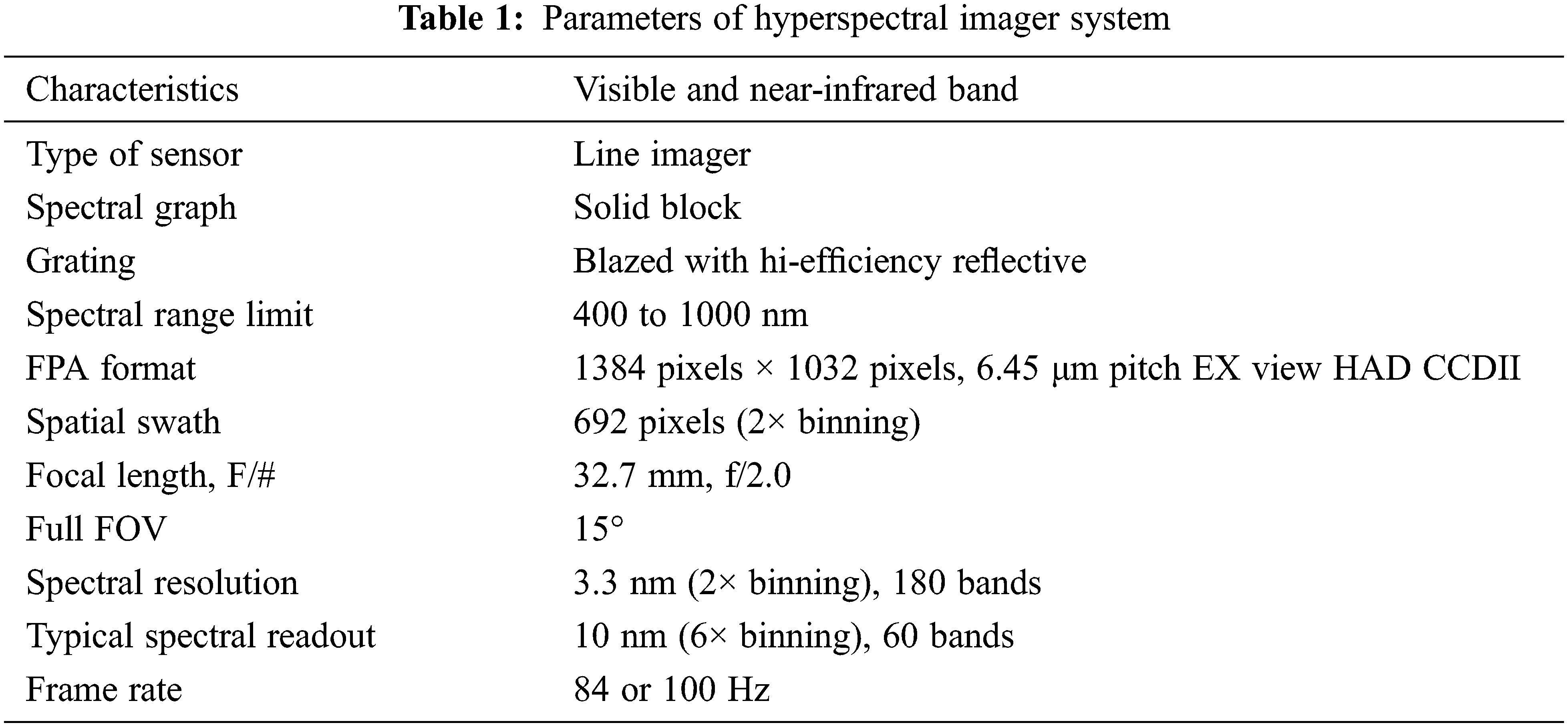
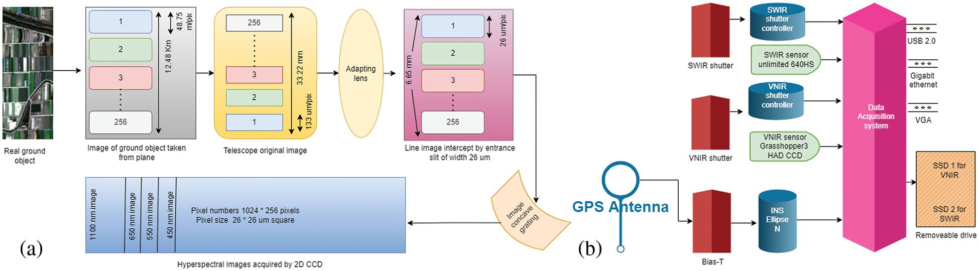
Figure 1: Block diagram of hyperspectral: (a) imager system, (b) data storage system

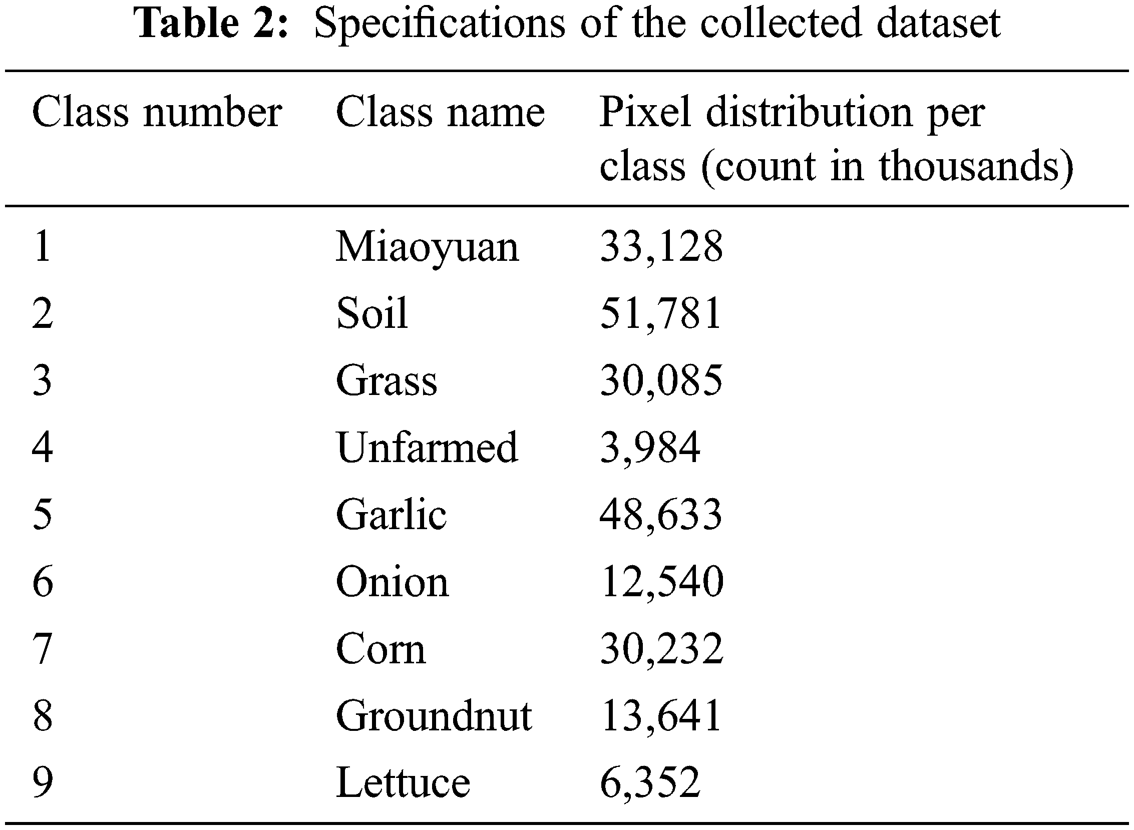
The Taiwan Agricultural Research Institute (TARI), Taiwan provided the ground truth for this research region in Quantum Geographic Information Systems (QGIS) data format with the local survey preceding the remote sensing by a one-month interval. The collected dataset from the study area has a 331 pixels × 696 pixels dimension with a total of 230,376 pixels and is composed of 9 distinct imbalance classes, as shown in Table 2. It is a high-resolution spectral dataset with 3.33 nm bandwidth in the selected VNIR range. The spatial resolution of the dataset is higher which is beneficial for academic research as well as real-world applications such as area mapping and classifier algorithm performance testing.

2.2 Geometric Correction

Geometric correction is performed to prevent geometric distortions caused by distorted images. This is accomplished by establishing a relationship between the image and the geographic coordinate system using sensor calibration, measured position, attitude data, ground control points, atmospheric conditions, etc. The Ellipse-N tiny INS with an integrated Global Navigation Satellite System (GNSS) receiver is used in this system. This lightweight sensor combines a Microelectromechanical System (MEMS)-based IMU with three gyroscopes and three accelerometers. It employs an upgraded Extended Kalman Filter (EKF) that combines inertial data with GNSS and Differential Global Positioning System (DGPS) information. The Ellipse-N provides position and attitude data 200 times per second. The navigation information linked with the moment of image capture is kept in two separate files before the image data is saved to the storage. First is a text file in which the navigation information having location and attitude data is recorded for each line of the image data.

2.3 Geo Referencing

The second is an Input Geometry (IGM) file of the Environment for Visualizing Images (ENVI) software which comprises the latitude and longitude of each pixel in the image. It includes an optimized process that will create geo-registered data while providing the image data and IGM script. Georeferenced image mapping information is recorded in two bands, one for x-coordinate (longitude or easting) and the other for y-coordinates (latitude or easting)/ (latitude or northing). Several bands of longitude and latitude are included with certain datasets which provide the georeferencing information for every raw pixel in the original raw image. The file is used to generate (on-the-fly) a Geographic Lookup Table (GLT) file that contains information about which starting pixel corresponds to which output pixel in the final image. It is possible to rectify distortions such as roll, pitch, and yaw effects using this form of geographical assessment premised on the flight track. Some datasets include specified geographical coordinates bands which are combined to form the IGM file. This file is not georeferenced itself, but it includes the georeferencing metadata for each source pixel. Following procedures must be executed to do geometric corrections on the HSI dataset.

• To begin, open the required VNIR image in ENVI Software.

• Select IGM’s geometric correction > geo-reference from the toolbox. The file dialogue for data input appears.

• After choosing an input file, execute the optional spectral sub-settings by selecting the appropriate IGM file, where band 2 and 1 contains x and y geometry coordinates, respectively.

• Choose the type of projection in the source perspective list of geometric bands. Select the georeferencing and generate GLT File parameter projection in degrees from the georeferencing outcome projection list to enter the output pixel size. If a north-up picture is desired, set the output rotation to zero. Change the filenames of the GLT and the output georeferenced files and save the picture.

2.4 Region of Interest Creation

Regions of Interest (ROI) are subsets of a raster designated for a specific reason which is the area of crops in this scenario. These are processed to derive categorization statistics. It is indicated which pixels of the image will be included or excluded from the ROI during its specification. After the geometric corrections, a region with a spatial dimension of 696 pixels × 331 pixels is created by using the coordinates indicated in Table 3. A new vector layer is created and transformed vector-shape file into an ROI by making a subset of this raster and masking the leftover pixels with zero values.

3  Methodology

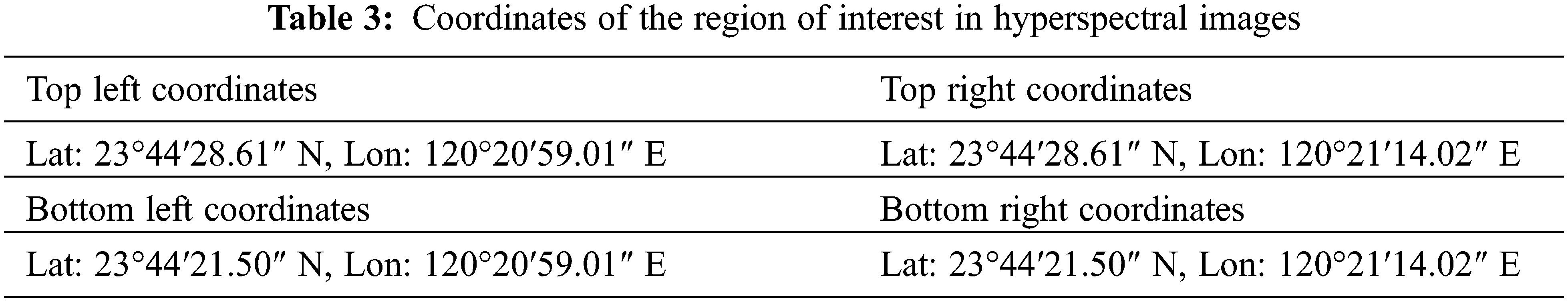
Fig. 2 depicts a broad diagram of the overall design of the experiment and the proposed scheme adopted for the multiclass classification of crops. The procedure of feature extraction and classification from the preprocessed data is explained below.

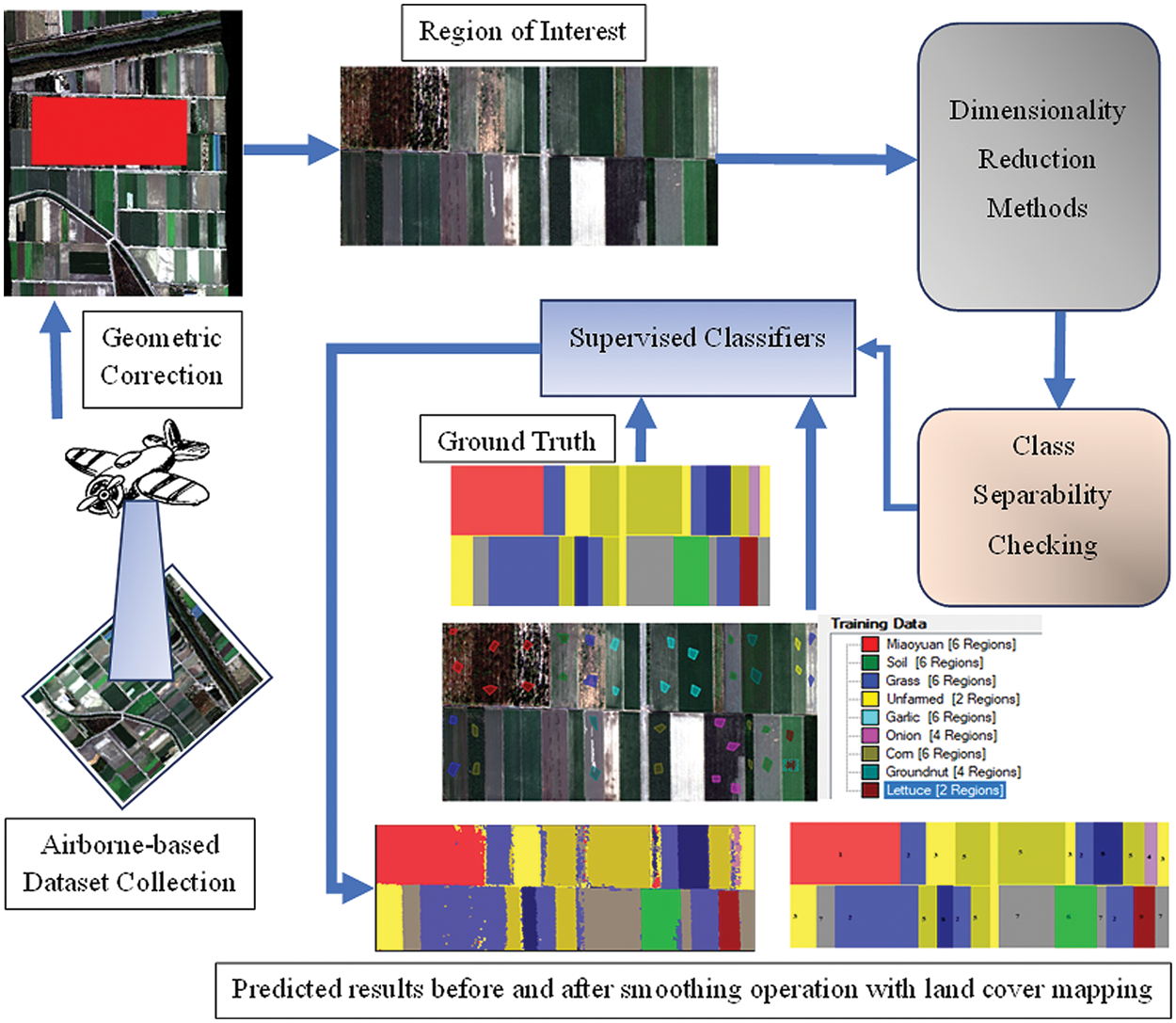
Figure 2: Experimental scheme and proposed approach for remote sensing

3.1 Edge-Preserving Filters

Edge preserving filtering is a technique for image processing that reduces the noise while keeping crucial parts of the image, such as borders and other visual cues. Over the last two decades, the image analysis and computer vision fields have paid a lot of attention to these methods. Hyperspectral remote sensing techniques have successfully used certain powerful edge-preserving filters [18,19]. It was used for the first time to make the best use of spectral and spatial information in the post-processing of pixel-wise categorization results [18]. This filtering technique is good for post-processing purposes, though it is not the best option. A method for isolating the smallest sections of the HSI is presented in [20] to further increase its interpretability. The image classification characteristics are enhanced using edge-preserving filtering and ensemble classifier after deconstructing the HSI with ICA.

Anisotropic diffusion and the bilateral filter in terms of edge preservation are the most used filters with high computational costs [21]. An iterative solution is required for anisotropic diffusion, in contrast to bilateral filtering, which employs a spatial variability weighting function. Although other methods for accelerating anisotropic diffusion or bilateral filtering have been developed, the bulk of these solutions are limited to grayscale pictures or rely on temporary procedures [22,23]. The guided filter [24], the domain transform filter [25], and the deep edge-aware filter [26] are other techniques for edge-preserving filtering. The domain morph recursive filter works in real-time and is particularly helpful in improving the performance of the HSI classifier [25]. In this work, the Domain Transform Recursive Filter (DTRF) is initially used to apply an estimated distance-conserving adjustment (a simple estimate is the sum of the spatial distance and the variation in brightness between each pixel).

Ui=Io+∑j=1i⁡(1+δsδr|Ij−Ij−1|) (1)

The notations δs and δr represents the procedure to change the degree of filter smoothness for the domain transformed signal denoted as U , and I denotes the one-dimensional (1D) signal used for DTRF. The input signal is then analyzed as follows via recursive filtering:

Ji=(1−ab)Ii+abJi−1 (2)

where Ji is the ith pixel’s filter result, a = exp ( −2/δs ) ∈ [0,1] is the feedback parameter, and b is the distance in the transform domain between two data points/samples Ui and Ui−1 . When b decreases, ab decreases to zero, completing the propagation cycle and recreating edges in the signal, and vice versa. This edge-preserving filter processed the image in 1D operation to reduce the computational cost and increase the processing time. According to experimental findings, a single pass of this 1D operation generates filtered pictures with no objects. Three passes of this 1D filtering are required to get the considerable edges in the 2D images. The DTRF is applied to the test images to obtain the edge-preserved filtered image (I,δs,δr) , where I represents the input band and δs and δr are smoothness adjustment parameters. Fig. 3 represents the procedure of the proposed PCA-EPF approach.

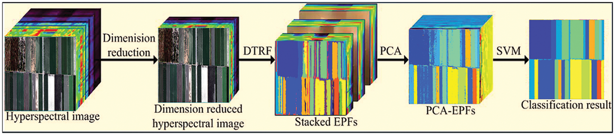
Figure 3: Illustrative diagram of the proposed PCA-EPF method

3.2 Principal Component Analysis

PCA is the fundamental technique for a wide range of remote sensing-based pattern recognition applications. It is simple, non-parametric, and effective to extract the key information from the HSI [17]. The PCA is used in this study for dimensionality reduction. The EPF generated by varying parameter values includes a significant amount of redundant information for which the PCA is the effective method to eliminate the redundancy. Image denoising effectively minimized the spectral variations between pixels of the same class along with the elimination of small information. This smoothing operation also decreased the distinction between pixels of the different classes which affects the classification performance. PCA is an excellent answer to this issue since it can extract the most critical features from the EPF stack while effectively highlighting spectral variations between the pixels of distinct classes.

The essential equation for PCA-based sparse representation is encoded in the data matrix S , which consists of N observations and M variables. In the image processing domain, N is the total number of pixels in an image, and M represents the values of each pixel feature.

P=W′S (3)

where P values are the main components built as a weighted average of the original sample vectors. The components in P are designed to conserve more variance discovered in the previous components. W is defined by the covariance matrix C :

W=EA−12 (4)

where A is a diagonal matrix containing the decreasing eigenvalues of C and E is a matrix containing the increasing eigenvectors of C . Given that the nth column of the M by N matrix B is SN−μ

B=[S1−μ,…,SN−μ] (5)

The average vector is found by plugging the numbers into the formula μ=(1/N)(S1+⋅⋅⋅+SN) . Covariance matrix C of size M×M may be found using the formula:

C=1N−1BBT (6)

From Eq. (4), it is deduced that W is a scaling factor for E vector-matrix, such that the variance of each independent variable Pm equals 1. Dimensions of the input data S are reduced by keeping the first L significant components. The proposed process defines the trained framework as PCA (S,L) where L is the number of components to hold from the data matrix S . This part explains the basic theory and PCA equations.

3.3 Spectral Dimensionality Reduction

A band averaging approach minimizes the hyperspectral dimensions. It reduces the computational cost of extraction function and image denoising of the original HSI. The hyperspectral M -dimensional data I is partitioned into K equal-sized subgroups along the spectral axis as I=I1,...,IK . K is the reduced dimensionality of the data corresponding to the number of bands. The final set of [M/K] bands in HSI is implemented by creating the K th subgroup if M is divisible by K . When M is indivisible by K then [M/K] is determined by the lowest integer which is greater than M/K number. It defines the number of bands in each subgroup. The resulting dimension-reduced hyperspectral data is the sum of the averages of the band subsets or I^K=I^1,...,I^k .

The reduced data retains sufficient detail of the original image in each pixel. This is a major advantage of using the average-based dimensionality reduction technique. The edges and other essential spatial structures in larger and separate components can be significantly distorted along with dimensionality reduction advantage using transform-based techniques such as ICA and PCA. As a result, the effectiveness of the subsequent edge-preserving filtering is decreased. The feature selection-based techniques may be adopted in addition to transform-based methods to overcome this issue, but they require an extensive optimization process. As shown in this study, a simple dimensionality reduction technique based on averaging function provides satisfactory classification performance.

3.4 Feature Extraction with EPF Stack

The EPF of HSI can be computed and overlaid with previously collected k-dimensional hyperspectral data as shown below.

Fkx=DTRF(I^K,δsx,…,δrx),x=1,…,X,k=1,…,K (7)

F={F1,…,FX} (8)

where δsx and δrx are the xth parameter specifications for a domain transform recursive filter. For the dimension-reduced kth band, the EPF is constructed with various parameter values (δsx,δrx)⊂{(δs1,δr1),…,(δsX,δrX)} . The generated features are then layered together following Eq. (8).

The main reason for this update is to capture the multi-scale spatial features already stored in EPF with suitable parameter values. As seen in Fig. 3, modifying the domain transforming recursive filter parameters might result in drastically different filtered images in terms of boundary and edge preservation. Excessive blurring may reduce the spectral separability of pixels from distinct objects. To cater to these issues, filtration with a significant level of smoothing may effectively decrease noise and increase the spectral retention of pixels. This indicates that EPF obtained with variable degrees of smoothing operation has benefits in representing certain objects or features at various scales. As a result, it is projected that combining these features would increase classification performance by using the supplementary data present in the stacked EPF.

The training process of the experimental setup is proceeded in two different approaches which are regarded as 1st and 2nd way of training, respectively, as illustrated in Fig. 4. The number of training samples are frequently changing from 1% to 10% and is randomly picked out of ground truth for 1st way of training mode in ten folds. While each new training fold includes a percentage of training samples from the previous experiment along with fresh randomly selected samples in the 2nd way of training.

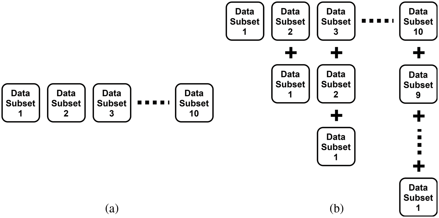
Figure 4: Training data adjustment for all ten experiments: (a) 1st way of training, (b) 2nd way of training

4  Results and Discussion

The SVM classifier is implemented for multiclass crop classification from the HSI dataset of the VNIR range. The dataset is further divided into ten distinct experimental configurations after the application of geometric correction, localization annotation, and other post-processing operations. This dataset division in experimental folds is based upon the pixel count values with consideration of each target or class variable. The distribution of these pixels for each arrangement of the experimental work has been shown in Fig. 5. The random dispersion of these pixels has been processed for each experimental arrangement with minor changes in the pixel count for each class present in the dataset. The class-wise data is further investigated as dimensionality reduced spectrum, stacked EPF spectrum, and PCA-EPF spectrum which is the PCA-based dimensionality reduced feature stack. The spectrum analysis of class “Garlic” has been investigated in Fig. 6 with the band number and the illuminance factor.

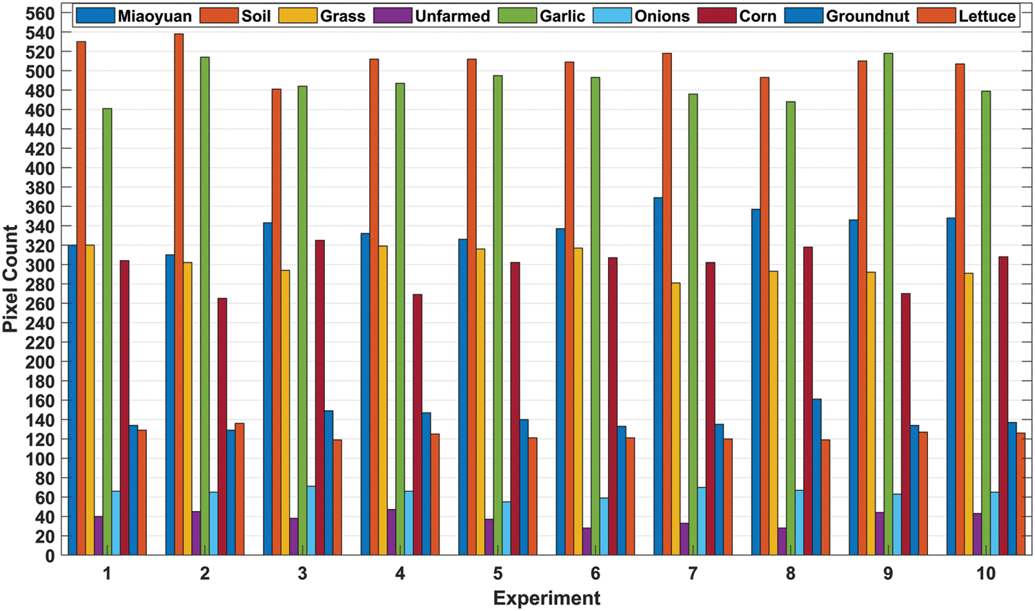
Figure 5: The number of pixels per class for all the ten experimental arrangements

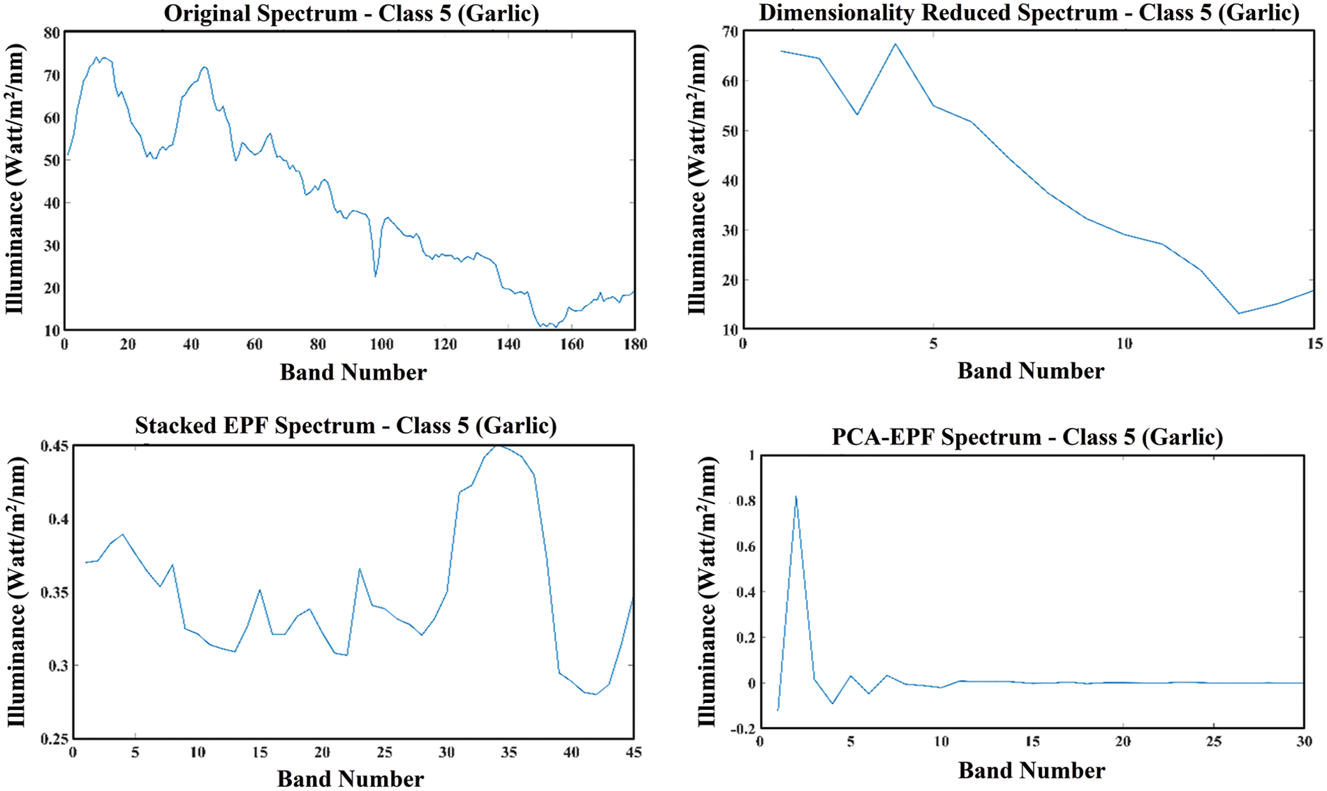
Figure 6: The spectral signatures of the “Garlic” class in the visible and near-infrared range

The effectiveness of the proposed scheme for crop classification is evaluated with the SVM classifier by utilizing two feature sets having the ordinary EPF stack and PCA-EPF stack, respectively. The classifier is trained for both feature sets with both ways of the training described previously. Various classification performance assessment metrics are computed for each feature set with each training method. The primary goal of this collected dataset is to develop state of the art in hyperspectral (non-RGB) categorization. This section will provide some benchmark results for future works in hyperspectral imaging-based crop classification in agricultural remote sensing. The accuracy of the classifier with the proposed methodology is measured in terms of the Average Accuracy (AA), Overall Accuracy (OA), and Cohen Kappa (CK) coefficient [27,28].

OA=1N(∑i=1P⁡ni) (9)

AA=1k(∑c=1k⁡Ac) (10)

CK=Po−Pm1−Pm (11)

Pm=1N2(∑k⁡nc1nc2) (12)

where N is the total number of samples, P is the total number of correct predictions, ni are total correct predictions for pixel i, k is the total number of classes, AC is the accuracy of class c , Po is overall accuracy, Pm is the probability of agreement between the correct predictions for two class pairs.

Fig. 7 represents the segmented ground truth class labels for each class along with pixel intensity mapping. Fig. 8 illustrates the image segmentation results with the SVM classifier applied for both feature sets. These results are obtained with the 1st way of training on pixel count-based three experimental dataset distributions. It is clearly shown that the results generated with the standard EPF stack originated many misclassifications due to the involvement of the salt and pepper noise in almost all the classes. While the segmentation performance shown by the PCA-EPF is comparatively improved but it still has errors and noise in comparison to the ground truth labels in Fig. 7.

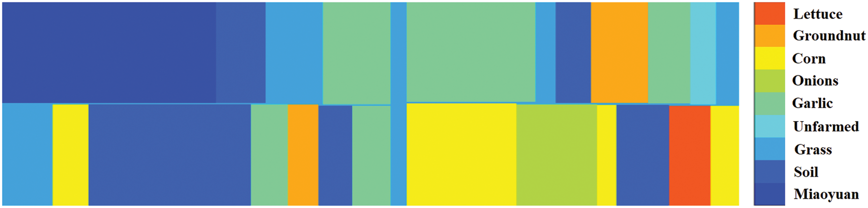
Figure 7: Ground truth class labels

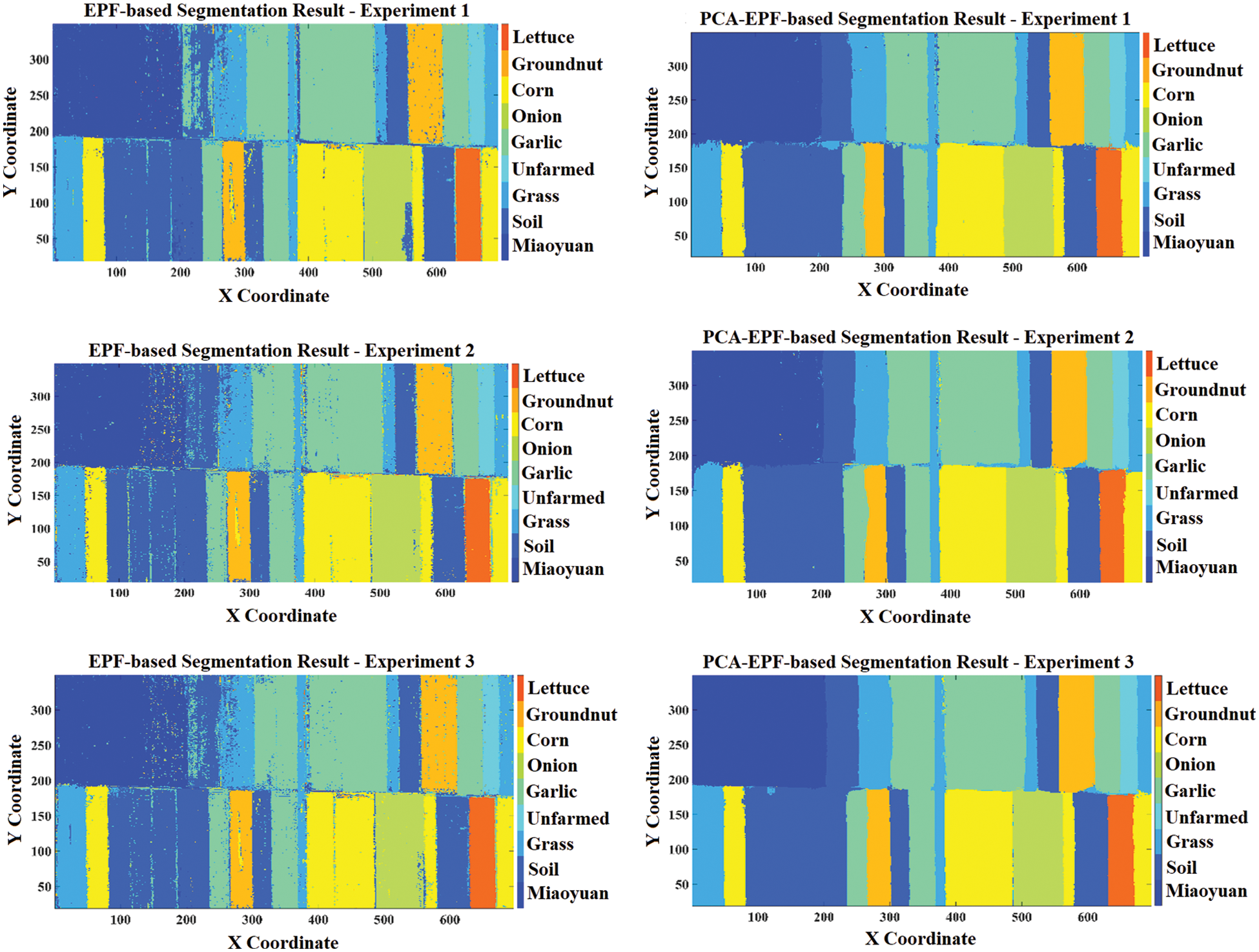
Figure 8: Comparative results of segmentation with both feature sets by using 1st way of training

An identical investigation has been generated with the 2nd way of training in which some percentage of the data from the preceding experiment is added up to the following experimental data. For example, the 1% data of experiment number 1 is added to the next 2% data to make the dataset (1% + 2%) for experiment number 2. Fig. 9 illustrates the image segmentation results on the nine classes using 2nd way of training for both feature sets in three experimental configurations. The 2nd way of training has also significantly improved the pixel-based classification results using PCA-EPF as compared to the original EPF stack against the ground truth labels of each class.

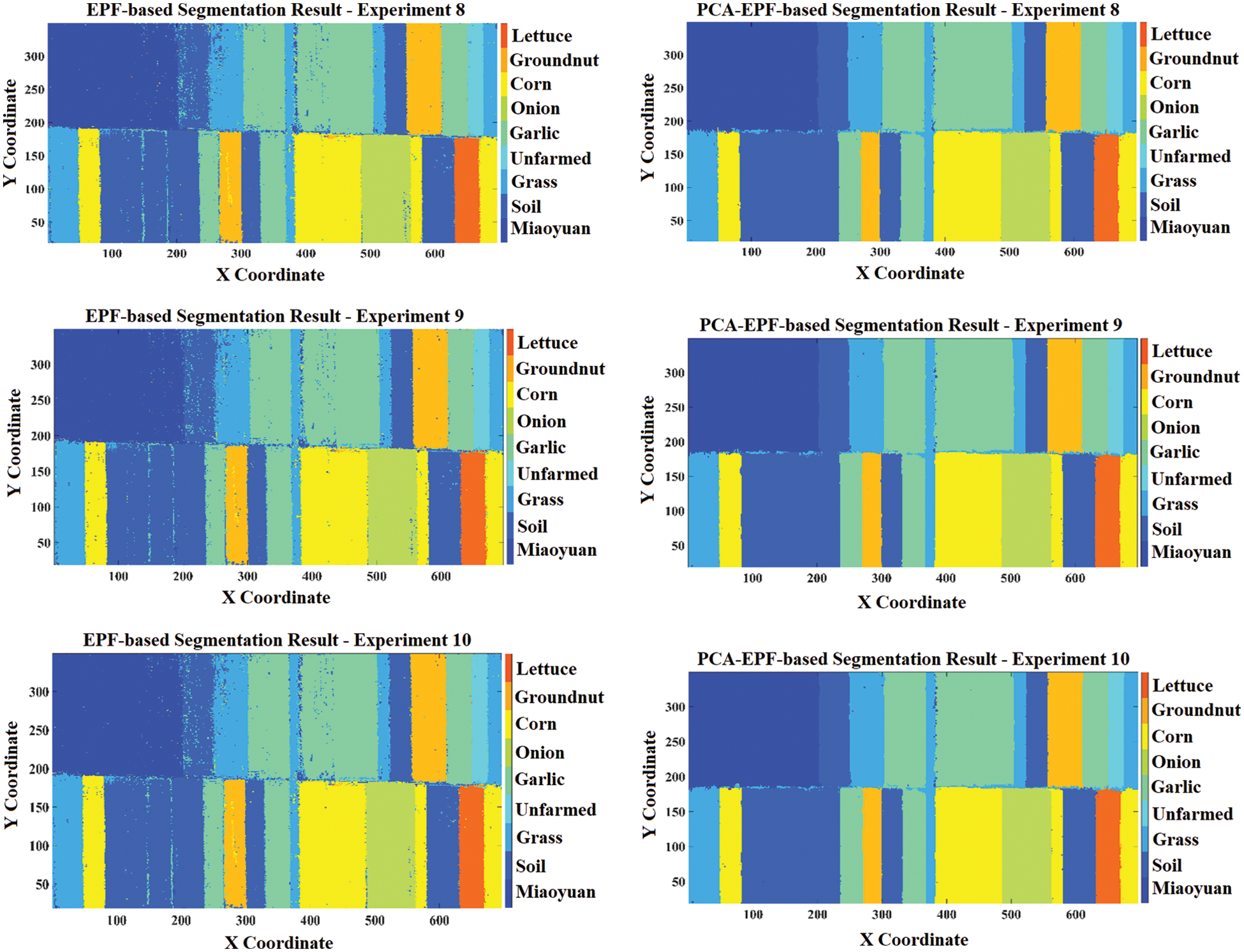
Figure 9: Comparative results of segmentation with both feature sets by using 2nd way of training

Fig. 10 represents the detailed classification results by using the EPF feature set with the first method of training. The performance assessment metrics for each experiment have been illustrated in Fig. 10a. All the metrics achieved more than 90% results in all the experiments, whereas the best scores were generated by experiment number 10 with 92.29% OA, 93.5% AA, and 90.84% CK. The class-wise accuracies of each class in all ten experiments have been shown in Fig. 10b. On average, all the classes are well classified with more than 88.6% accuracy, whereas class 1 (Miaoyuan) achieved the best classification accuracy of 96.49%. Similarly, Fig. 11 represents the detailed classification results by using the EPF feature set with the second method of training. All the performance assessment metrics achieved more than 90% results in all the experiments, whereas the best scores are generated by experiment number 10 with 95.13% OA, 95.66% AA, and 94.21% CK as shown in Fig. 11a. On average, all the classes are well classified with more than 90.83% accuracy, whereas the class 6 (Onion) achieved the best classification accuracy of 97.95% as shown in Fig. 11b. The comparative analysis of both ways of training reveals that the 2nd way of training achieved better results while employing the original EPF feature stack for the crop classification.

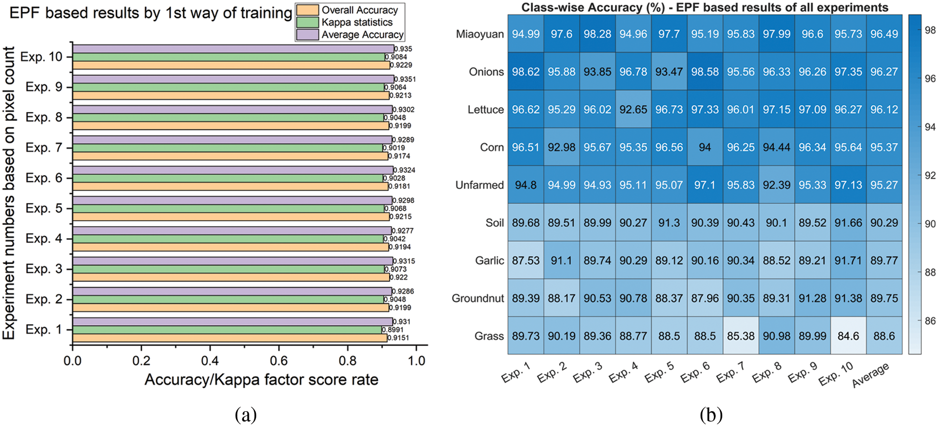
Figure 10: Classification with the original feature set and 1st way of training: (a) Average and overall accuracy, kappa statistics, (b) Class-wise accuracy for crop classification

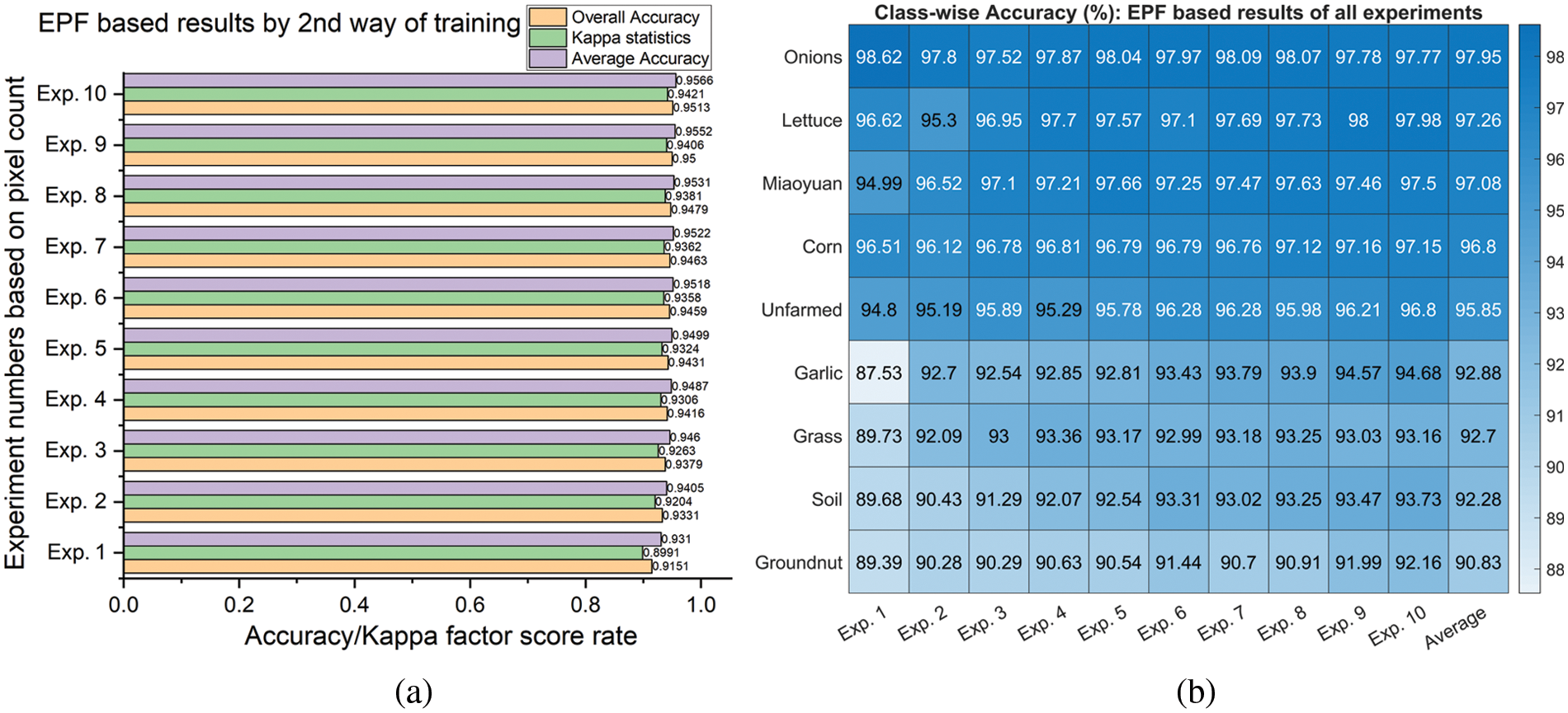
Figure 11: Classification with the original feature set and 2nd way of training: (a) Average and overall accuracy, kappa statistics, (b) Class-wise accuracy for crop classification

A similar approach is carried out for classification with the dimensionality reduced PCA-EPF feature set using both ways of training. The classification results and performance assessment are shown in Fig. 12. All the performance assessment metrics achieved more than 96% results in all the experiments, whereas the best scores are generated by experiment number 8 with 97.24% OA, 97.23% AA, and 96.72% CK as shown in Fig. 12a. On average, all the classes are well classified with more than 93.89% accuracy, whereas the class 9 (Lettuce) achieved the remarkable classification accuracy of 99.25% as shown in Fig. 11b. The comparative analysis and comprehensive conclusion of the results show that the PCA-EPF feature set has significantly improved the crop classification performance of the SVM classifier as compared to the EPF feature stack. It has outperformed previous experimental results with an additional pixel count adjustment for experiment number 8. It is observed that different training approaches for this feature set have not revealed any noticeable differences in the results.

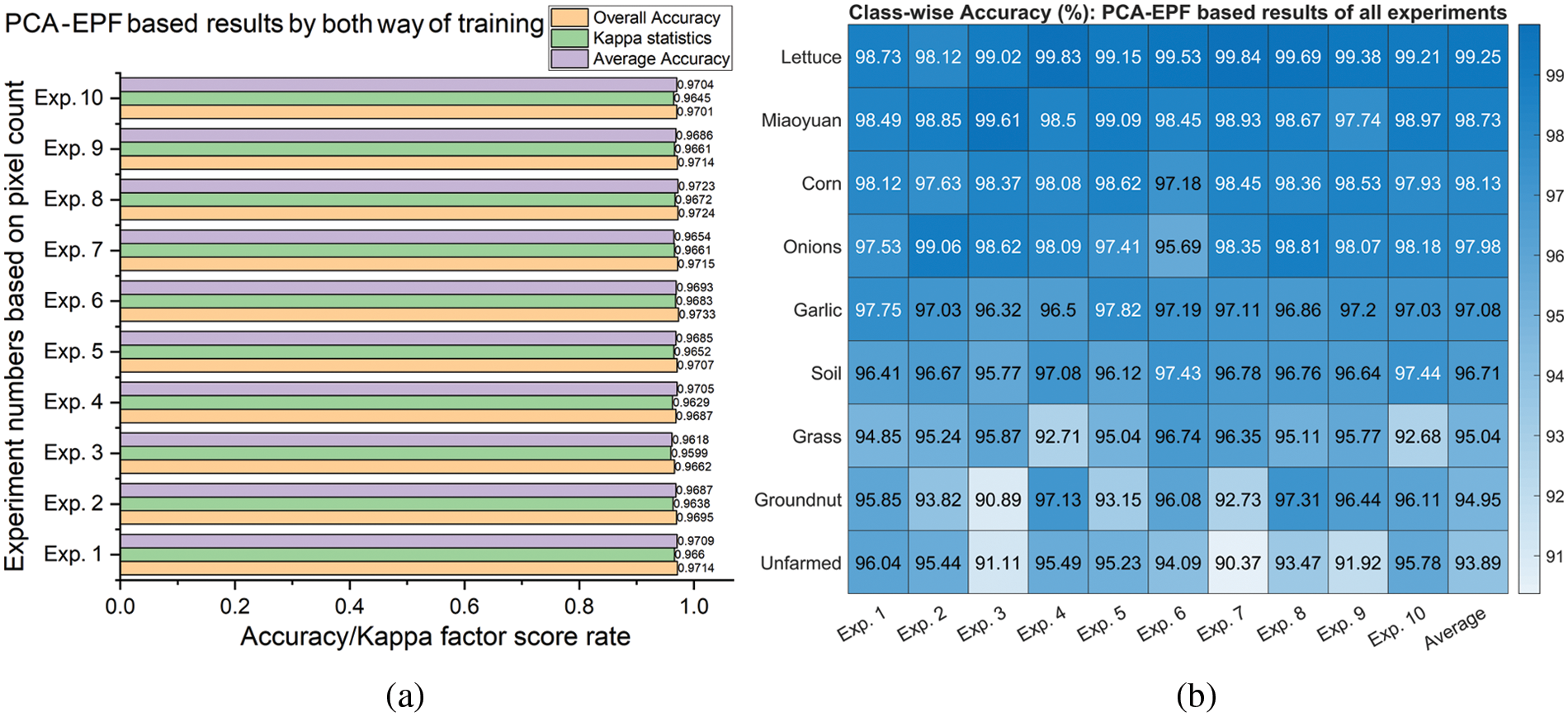
Figure 12: Classification with dimensionality reduced feature set using 1st and 2nd way of training: (a) Average and overall accuracy, kappa statistics, (b) Class-wise accuracy for crop classification

PCA-based approaches have been used with multiple remote sensing datasets and machine learning classifiers in similar studies. The PCA was used for the cannabis plant detection in [29]. It is employed to eliminate superfluous spectral data from multiband datasets. This study only focused on the detection of the plants without any detailed analysis and the use of the classification method. The authors implemented multiple PCA-based methodologies for the classification of HSI-based remote sensing data in [30]. The best approach was a minimum noise fraction with less than 98% accuracy and 97% CK. In [31], the PCA estimation method based on a geographical construction approach (gaPCA) is presented. It is an alternative for computing the main components using a geometrically constructed approximation of the PCA. The study used the SVM in combination with traditional PCA and gaPCA for its application to HSI-based remote sensing. This approach attains 96% accuracy and 95% CK. The proposed PCA-EPF approach in this study achieved the best results with greater than 98% accuracy and 97.14% kappa factor.

5  Conclusions

In this work, a unique pixel-based approach is proposed and implemented to perform the crop classification from hyperspectral remote sensing data of agricultural land by using Principal Component Analysis-based Edge Preserving Features (PCA-EPF). In methodology, the edge-preserving filtering with manually adjusted parameters is performed on hyperspectral images (HSI) of spectrally reduced dimensions to extract the standard EPF stack. These extracted features are treated with PCA to illustrate the stack in the mean square sense and to highlight the spectral differences among various classes. For crop classification, the support vector machines classifier is used with the PCA-EPF to classify the hyperspectral data in the visible and near-infrared (VNIR) range of 400–1000 nm wavelengths. The remarkable classification results with less computational cost are achieved for assessment metrics like individual class accuracy, average accuracy, overall accuracy, and kappa factor. The comparison with existing studies has shown that the proposed scheme outperforms the existing methods with up to 99% accuracy for agricultural target classification. As short-wave infrared (SWIR) data is also acquired with VNIR, future research directions are to use the features from SWIR data and data fusion of both ranges. Designing an automatic smoothing parameter selection approach to improve the classification accuracy for the hyperspectral dataset would be interesting future work.

Acknowledgement: Princess Nourah bint Abdulrahman University Researchers Supporting Project number (PNURSP2022R51), Princess Nourah bint Abdulrahman University, Riyadh, Saudi Arabia.

Funding Statement: Princess Nourah bint Abdulrahman University Researchers Supporting Project number (PNURSP2022R51), Princess Nourah bint Abdulrahman University, Riyadh, Saudi Arabia.

Conflicts of Interest: The authors declare that they have no conflicts of interest to report regarding the present study.

References

 1.  Y. Liu, G. Gao and Y. Gu, “Tensor matched subspace detector for hyperspectral target detection,” IEEE Transactions on Geoscience and Remote Sensing, vol. 55, no. 4, pp. 1967–1974, 2016. [Google Scholar]

 2.  S. Li, K. Zhang, Q. Hao, P. Duan and X. Kang, “Hyperspectral anomaly detection with multiscale attribute and edge-preserving filters,” IEEE Geoscience and Remote Sensing Letters, vol. 15, no. 10, pp. 1605–1609, 2018. [Google Scholar]

 3.  F. Kizel, M. Shoshany, N. S. Netanyahu, G. Even-Tzur and J. A. Benediktsson, “A stepwise analytical projected gradient descent search for hyperspectral unmixing and its code vectorization,” IEEE Transactions on Geoscience and Remote Sensing, vol. 55, no. 9, pp. 4925–4943, 2017. [Google Scholar]

 4.  J. Li, I. Dópido, P. Gamba and A. Plaza, “Complementarity of discriminative classifiers and spectral unmixing techniques for the interpretation of hyperspectral images,” IEEE Transactions on Geoscience and Remote Sensing, vol. 53, no. 5, pp. 2899–2912, 2014. [Google Scholar]

 5.  T. Lu, S. Li, L. Fang, L. Bruzzone and J. A. Benediktsson, “Set-to-set distance-based spectral-spatial classification of hyperspectral images,” IEEE Transactions on Geoscience and Remote Sensing, vol. 54, no. 12, pp. 7122–7134, 2016. [Google Scholar]

 6.  B. Sun, X. Kang, S. Li and J. A. Benediktsson, “Random-walker-based collaborative learning for hyperspectral image classification,” IEEE Transactions on Geoscience and Remote Sensing, vol. 55, no. 1, pp. 212–222, 2016. [Google Scholar]

 7.  S. Arif, M. Arif, S. Munawar, Y. Ayaz, M. J. Khan et al., “EEG spectral comparison between occipital and prefrontal cortices for early detection of driver drowsiness,” in IEEE Int. Conf. on Artificial Intelligence and Mechatronics Systems (AIMS), Bandung, Indonesia, pp. 1–6, 2021. [Google Scholar]

 8.  G. Cheng, J. Han, L. Guo, Z. Liu, S. Bu et al., “Effective and efficient midlevel visual elements-oriented land-use classification using VHR remote sensing images,” IEEE Transactions on Geoscience and Remote Sensing, vol. 53, no. 8, pp. 4238–4249, 2015. [Google Scholar]

 9.  G. Cheng, J. Han and X. Lu, “Remote sensing image scene classification: Benchmark and state of the art,” Proceedings of the IEEE, vol. 105, no. 10, pp. 1865–1883, 2017. [Google Scholar]

10. G. Licciardi, P. R. Marpu, J. Chanussot and J. A. Benediktsson, “Linear versus nonlinear PCA for the classification of hyperspectral data based on the extended morphological profiles,” IEEE Transactions on Geoscience and Remote Sensing Letters, vol. 9, no. 3, pp. 447–451, 2011. [Google Scholar]

11. Y. Chen, N. M. Nasrabadi and T. D. Tran, “Hyperspectral image classification using dictionary-based sparse representation,” IEEE Transactions on Geoscience and Remote Sensing, vol. 49, no. 10, pp. 3973–3985, 2011. [Google Scholar]

12. L. Fang, S. Li, X. Kang and J. A. Benediktsson, “Spectral-spatial classification of hyperspectral images with a superpixel-based discriminative sparse model,” IEEE Transactions on Geoscience and Remote Sensing, vol. 53, no. 8, pp. 4186–4201, 2015. [Google Scholar]

13. S. Arif, M. J. Khan, N. Naseer, K. S. Hong, H. Sajid et al., “Vector phase analysis approach for sleep stage classification: A functional near-infrared spectroscopy-based passive brain-computer interface,” Frontiers in Human Neuroscience, vol. 15, no. 658444, pp. 1–15, 2021. [Google Scholar]

14. A. Villa, J. A. Benediktsson, J. Chanussot and C. Jutten, “Hyperspectral image classification with independent component discriminant analysis,” IEEE Transactions on Geoscience and Remote Sensing, vol. 49, no. 12, pp. 4865–4876, 2011. [Google Scholar]

15. J. Zabalza, J. Ren, Z. Wang, H. Zhao, J. Wang et al., “Fast implementation of singular spectrum analysis for effective feature extraction in hyperspectral imaging,” IEEE Journal of Selected Topics in Applied Earth Observations and Remote Sensing, vol. 8, no. 6, pp. 2845–2853, 2014. [Google Scholar]

16. D. Lunga, S. Prasad, M. M. Crawford and O. Ersoy, “Manifold-learning-based feature extraction for classification of hyperspectral data: A review of advances in manifold learning,” IEEE Signal Processing Magazine, vol. 31, no. 1, pp. 55–66, 2013. [Google Scholar]

17. X. Kang, X. Xiang, S. Li and J. A. Benediktsson, “PCA-based edge-preserving features for hyperspectral image classification,” IEEE Transactions on Geoscience and Remote Sensing, vol. 55, no. 12, pp. 7140–7151, 2017. [Google Scholar]

18. X. Kang, S. Li and J. A. Benediktsson, “Spectral-spatial hyperspectral image classification with edge-preserving filtering,” IEEE Transactions on Geoscience and Remote Sensing, vol. 52, no. 5, pp. 2666–2677, 2013. [Google Scholar]

19. B. Pan, Z. Shi and X. Xu, “Hierarchical guidance filtering-based ensemble classification for hyperspectral images,” IEEE Transactions on Geoscience and Remote Sensing, vol. 55, no. 7, pp. 4177–4189, 2017. [Google Scholar]

20. J. Xia, L. Bombrun, T. Adali, Y. Berthoumieu and C. Germain, “Spectral-spatial classification of hyperspectral images using ICA and edge-preserving filter via an ensemble strategy,” IEEE Transactions on Geoscience and Remote Sensing, vol. 54, no. 8, pp. 4971–4982, 2016. [Google Scholar]

21. C. Liu and M. Pang, “One-dimensional image surface blur algorithm based on wavelet transform and bilateral filtering,” Multimedia Tools and Applications, vol. 80, no. 19, pp. 28697–28711, 2021. [Google Scholar]

22. M. Gharbi, J. Chen, J. T. Barron, S. W. Hasinoff and F. Durand, “Deep bilateral learning for real-time image enhancement,” ACM Transactions on Graphics (TOG), vol. 36, no. 4, pp. 1–12, 2017. [Google Scholar]

23. S. Pan, X. An and H. He, “Optimal O(1) bilateral filter with arbitrary spatial and range kernels using sparse approximation,” Mathematical Problems in Engineering, vol. 2014, no. 289517, pp. 1–11, 2014. [Google Scholar]

24. S. Li, X. Kang and J. Hu, “Image fusion with guided filtering,” IEEE Transactions on Image processing, vol. 22, no. 7, pp. 2864–2875, 2013. [Google Scholar]

25. E. S. Gastal and M. M. Oliveira, “Domain transform for edge-aware image and video processing,” ACM Transactions on Graphics, vol. 30, no. 4, pp. 1–12, 2011. [Google Scholar]

26. D. Cheng, G. Meng, S. Xiang and C. Pan, “FusionNet: Edge aware deep convolutional networks for semantic segmentation of remote sensing harbor images,” IEEE Journal of Selected Topics in Applied Earth Observations and Remote Sensing, vol. 10, no. 12, pp. 5769–5783, 2017. [Google Scholar]

27. T. Akhtar, S. O. Gilani, Z. Mushtaq, S. Arif, M. Jamil et al., “Effective voting ensemble of homogenous ensembling with multiple attribute-selection approaches for improved identification of thyroid disorder,” Electronics, vol. 10, no. 23, pp. 1–23, 2021. [Google Scholar]

28. T. Akhtar, S. Arif, Z. Mushtaq, S. O. Gilani, M. Jamil et al., “Ensemble-based effective diagnosis of thyroid disorder with various feature selection techniques,” in 2nd IEEE Int. Conf. of Smart Systems and Emerging Technologies (SMARTTECH), Riyadh, Saudi Arabia, pp. 14–19, 2022. [Google Scholar]

29. C. Gambardella, R. Parente, A. Ciambrone and M. Casbarra, “A principal components analysis-based method for the detection of cannabis plants using representation data by remote sensing,” Data, vol. 6, no. 10, pp. 1–13, 2021. [Google Scholar]

30. M. P. Uddin, M. A. Mamun and M. A. Hossain, “PCA-based feature reduction for hyperspectral remote sensing image classification,” IETE Technical Review, vol. 38, no. 4, pp. 377–396, 2020. [Google Scholar]

31. A. L. Machidon, F. D. Frate, M. Picchiani, O. M. Machidon and P. L. Ogrutan, “Geometrical approximated principal component analysis for hyperspectral image analysis,” Remote Sensing, vol. 12, no. 11, pp. 1–23, 2020. [Google Scholar]