
 Submit a Paper
 Propose a Special lssue
 Open Access
ARTICLE

Constructing an AI Compiler for ARM Cortex-M Devices
Department of Computer Science and Information Engineering, National Chung Cheng University, Chia-Yi, Taiwan
* Corresponding Author: Tam-Van Hoang. Email:
Computer Systems Science and Engineering 2023, 46(1), 999-1019. https://doi.org/10.32604/csse.2023.034672
Received 23 July 2022; Accepted 13 November 2022; Issue published 20 January 2023
 View Full Text
 Download PDF
Abstract
The diversity of software and hardware forces programmers to spend a great deal of time optimizing their source code, which often requires specific treatment for each platform. The problem becomes critical on embedded devices, where computational and memory resources are strictly constrained. Compilers play an essential role in deploying source code on a target device through the backend. In this work, a novel backend for the Open Neural Network Compiler (ONNC) is proposed, which exploits machine learning to optimize code for the ARM Cortex-M device. The backend requires minimal changes to Open Neural Network Exchange (ONNX) models. Several novel optimization techniques are also incorporated in the backend, such as quantizing the ONNX model’s weight and automatically tuning the dimensions of operators in computations. The performance of the proposed framework is evaluated for two applications: handwritten digit recognition on the Modified National Institute of Standards and Technology (MNIST) dataset and model, and image classification on the Canadian Institute For Advanced Research and 10 (CIFAR-10) dataset with the AlexNet-Light model. The system achieves 98.90% and 90.55% accuracy for handwritten digit recognition and image classification, respectively. Furthermore, the proposed architecture is significantly more lightweight than other state-of-the-art models in terms of both computation time and generated source code complexity. From the system perspective, this work provides a novel approach to deploying direct computations from the available ONNX models to target devices by optimizing compilers while maintaining high efficiency in accuracy performance.Keywords
Compilers have been developed and used for the past 50 years [1] to generate device-dependent executable binary files from high-level programming languages such as C and C++. However, the development of compilers has remained an area of active research due to the rapid proliferation of new hardware architectures and programming models [2]. In this field, particular challenges are posed by the complexity of modern compilers such as Low-Level Virtual Machine (LLVM) [3] and Tensor Virtual Machine (TVM) [4], as well as increasing concerns over the ability of compilers to port Open Neural Network Exchange (ONNX) [5] models to embedded systems without losing the accuracy of those models. Furthermore, the process of compiling ONNX models to generate the final binary files can be complicated and inflexible.
In compilers, optimization can be applied to the front-end, intermediate representation (IR), or backend. Optimizing the compiler parameters, such as those governing loop unrolling, register allocation, or code generation, is another approach. The performance of an optimization strategy can be measured by its impact on the execution time, code size, energy cost, or, in the case of neural network compilers, the information loss [6]. The main focus has been on backend compiler optimization methods, such as scheduling, resource allocation [7], and code generation. More holistic approaches to optimization [8] have not yet been well explored. Many backends have been developed to compile for different targets, for example a compiler autotuning framework using a Bayesian network [9]. This study focuses on building a Bayesian network for an ARM system with support from the GNU Compiler Collection (GCC) compiler. The studies in [10,11] focused on optimizing energy consumption in embedded systems and assessed the impact of the available compilers for multi-core processors. Another state-of-the-art compiler is DisGCo [12], which is mainly used for distributed systems. The LLVM and TVM compilers are also widely used for ONNX models. However, the mapping of operators in these two compilers to operators in ONNX is highly complex (e.g., LLVM mainly supports the multiplier accumulator operators). Therefore, the end users need a conversion step when computing with the fine-grained operators (e.g., convolution operators) that exist in most current ONNX models. Intuitively, this complexity makes the goal of maintaining the accuracy of ONNX models challenging when compiling for multiple hardware platforms. The problem becomes critical on embedded devices because their storage and computational resources are limited. The challenges faced by the previous approaches can be summarized as follows.
1. User applications written in standard machine learning frameworks such as the LLVM and TVM compilers require efficient hardware with high-performance computational power to produce quick and accurate results. Additionally, the process of compiling ONNX models to the C++ files directly to deploy applications on ARM devices is complex for users.
2. The key metrics for embedded machine learning applications focus on accuracy, power consumption, throughput/latency, and cost. Compiling an ONNX model into another format to improve the accuracy over existing compilers in ARM devices, while minimizing power usage, time, and cost, is a complicated task.
Therefore, in this work, a novel AI backend is proposed to solve these challenges faced by existing compilers. In contrast to previous approaches, a novel backend is developed for the ONNC, including optimized techniques to reduce the operator dimension for computing on a small device. These include techniques such as preprocessing the input image, tuning the dimension of the operators in the ONNX model, and tuning the execution function and padding (Pad) parameter in computations. The input to the backend consists of ONNX models, while the outputs are C++ files. Using the Cortex-M backend, application developers can take advantage of the high-level programmability aspects of C++ to run their next computations while compiling the ONNX models. Although the backend is developed for the platform of the ARM Cortex-M device, it is believed that this backend can be extended to generate code for other domain-specific languages. To the best of the authors’ knowledge, using a machine learning-based backend of the compiler to implement computations directly from the ONNX model to a device is the first attempt of its kind, specifically on the ARM Cortex-M device.
To summarize, the main contributions of this paper are as follows:
1. The main shortcomings of existing compilers are identified, and the development of a novel code generation process in ONNC is discussed. This process can directly compute the ONNX model on the target device.
2. A novel backend is developed for the ONNC compiler, called the CortexM backend, the simplest backend for a functional programming language to date. The backend plays an important role in creating the execution files while minimizing the impact on the accuracy of the ONNX models.
3. A set of optimizations is implemented both in the ONNX models and the CortexM backend to improve the performance of the system and maintain the accuracy of the ONNX models.
4. Two experiments, on handwritten digit recognition and image classification, are performed with the CortexM backend and compared with the results from other state-of-the-art methods to evaluate the benefits of this backend. Evaluation of the results shows that the backend obtains superior results, demonstrating its usefulness in the embedded system.
The remainder of this paper is organized as follows. Section 2 presents a compiler framework used to build the CortexM backend for the target device. Section 3 presents the system design to deploy an actual application involving the backend. Section 4 describes the experimental methodology. Section 5 gives the results of the experiments and compares them with other state-of-the-art research. The paper is concluded in Section 6.
This section gives an overview of the ONNC compiler framework architecture which is used to build the CortexM backend, with a discussion of the main compilation phases and the compilation workflow of a backend in the ONNC compiler. A brief outline of the core parts of the new backend is presented, including the data structure of a use-define chain in a tensor and the mapping of ONNX IRs to ONNC IRs.
2.1 Compiler Framework Architecture
The compiler framework uses the ONNC compiler introduced in [13], a neural network compiler consisting of a front-end, middle-end, and backend. The front-end translates the ONNX models into a low-level intermediate language, called ONNX IR. ONNX IR is an assembly-level language, and operands of all computational operations were built in ONNC IR.
The middle-end contains the ONNC IR and automatically finds the corresponding ONNX IR to create a machine instruction. The backend maps ONNC IRs to ONNX IRs one-to-one by their values, which simplifies computations of the ONNX model with ONNC backends. In ONNC compiler has four main compilation phases, which can be thought of as the core architecture of the ONNC compiler. Fig. 1 depicts the overview compilation framework architecture for the proposed backend. This architecture is the top-level block in the ONNC compiler, and it is also the order of compilation the backend uses to create the hardware binaries. Fig. 1 depicts the main compilation phases in the backend; all backends in ONNC use these four phases to compile an ONNX model. The phases are (1) addTensorSel, which triggers ONNC to invoke the name of a backend and translates ONNX IR to ONNC IR; (2) addTensorSched, which causes ONNC to schedule operators in topological order to improve performance; (3) addMemAlloc, which adds passes for allocating memory space for tensors; and (4) addCodeEmit, which registers the CodeEmit function for ONNC to generate executable code for the target device.
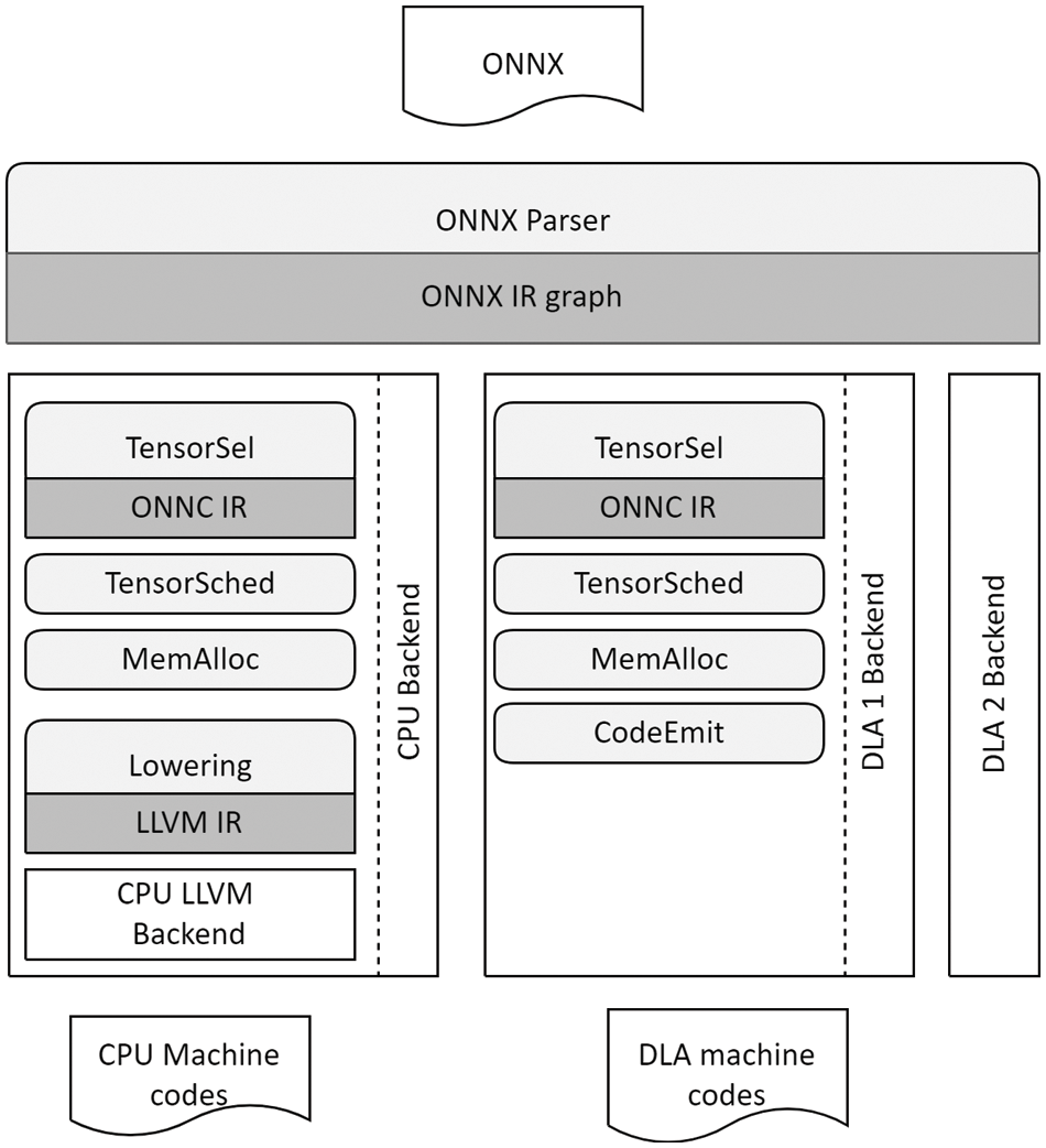
Figure 1: The compilation framework architecture
2.2 Compilation Workflow of the Backend
This section describes the workflow of a backend in the ONNC compiler. All operators in the ONNX model are mapped to the ONNC IRs. This mapping is implemented by a structure called the use-define chain in ONNC. Its main purpose is to create the relationship between a network graph and a computation graph in an ONNC backend.
2.2.1 The Data Structure of the Use-Define Chain
In the neural network, each layer is called an operator. All computation formulas in the same layer are the same; however, the input and output values are different. The computation of a convolution layer in ONNC is illustrated in Fig. 2. The operator
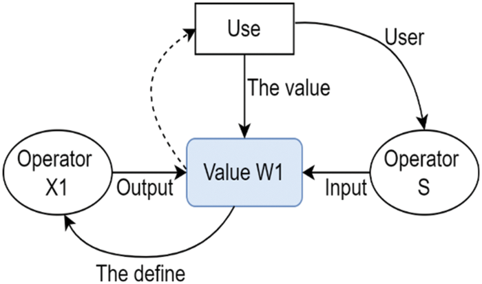
Figure 2: The data structure diagram of an operator’s use-define chain in ONNC, which is used to implement the mapping process from ONNX IRs to ONNC IRs
For example, the
2.2.2 The Mapping of ONNX IRs to ONNC IRs
As shown in Fig. 1, the input is the ONNX model and the output comprises the corresponding hardware binaries. This is similar to traditional compilation frameworks. However, the proposed compilation framework is simpler than other compilation frameworks in connecting the ONNX models to deep learning accelerators. Fig. 3 shows the mapping structure between ONNX IRs and ONNC IRs: at the top are the nodes in the ONNX model and at the bottom are the compute operators in ONNC. The “Inputs <*>” and “Outputs <*>” elements are the abstract classes of each node in ONNX and each operator in the ONNC compiler, respectively. Input and output are containers used to point out the input and output values of a particular operator. Since operators are inherited from the definer discussed in Section 2.2.1, it has a pointer to their values and this value is the value of the tensors. All ONNX IR operators are mapped to ONNC IRs by their values. The connections between these corresponding IR values are represented by the two red lines in Fig. 3.
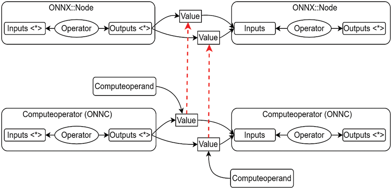
Figure 3: The value mapping process of the operators between ONNX IRs and ONNC IRs. The ONNC IRs find the corresponding values in ONNX IRs to link together
2.2.3 Compilation Flow of the Backend
The execution of a backend in ONNC is made up of four compilation phases, called IRReader, TensorSel, MemAlloc, and CodeEmit. The detailed compilation workflow of each phase is shown in Fig. 4. It consists of two parts, called the graph IR and compute IR. The graph IR consists of the original ONNX IRs that are used to represent the tensors in the ONNX models. The compute IR consists of the ONNC IRs and it is defined in ONNC. Its execution is as follows. In the TensorSel phase, ONNC maps to these ONNX IRs to translate into the compute IR part of the compiler and it selects corresponding instructions to generate the tensor, which is represented by symbols for target devices. In fact, both symbols of ONNX IR and the ONNC IR are the values of operands. In the MemAlloc phase, symbolic operands are turned into memory address, instruction scheduling, memory partition, and memory allocation. Finally, in the CodeEmit phase, it emits codes for target devices.
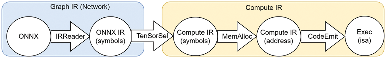
Figure 4: The compilation flow diagram of a backend with an ONNX model
This section describes the implementation of a specific application with the new backend. Because the goal is to deploy on Cortex-M devices, the execution diagram for this device is shown in Fig. 5—the same implementation flow was used for all experiments in the paper. It consists of four main phases. The first phase is to construct input data. The second phase builds the backend and adds the dimension-reduction techniques for operators and their corresponding parameters. The main goal of this phase is to make the input data suitable for the memory space of the target device. The third phase obtains the output results after the compilation process. The fourth phase is to deploy results on the specific application.
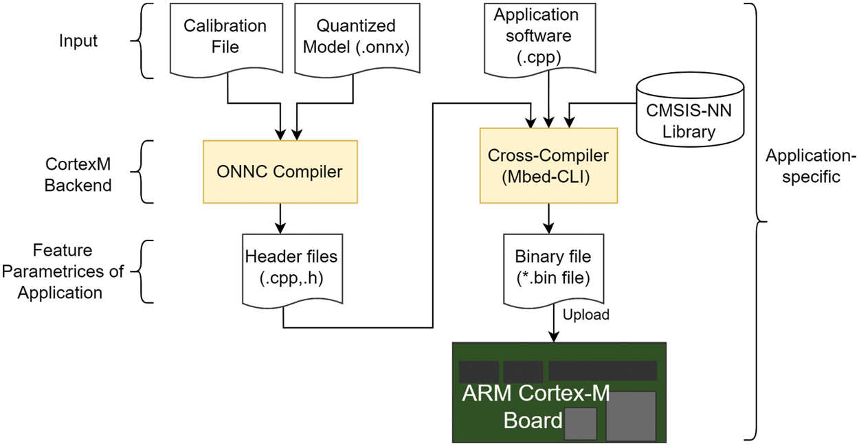
Figure 5: An overview block diagram of the system on the ARM Cortex-M board
Based on the target devices, choosing suitable input data is necessary to identify the best pre-processing phases while maintaining the accuracy of the ONNX model. In addition, optimizing to reduce the model size is necessary to match the model size with the target device. Because the features of the model are affected by optimization, a calibration file for the CortexM backend was used to store the right-shift information of the computed weight values. The details of calibration and the ONNX optimization follow.
The computation operations of the ONNX models with the Cortex Microcontroller Software Interface Standard Neural Network (CMSIS-NN) library are difficult to use immediately due to different data formats. In ONNX, the floating-point type is a common format that exceeds the computing range of the CMSIS-NN library, while the q7_t type in the CMSIS-NN library is a signed 8-bit type with the computation range (−128, 127). Therefore, memory overflow occurs on the embedded devices during the computation of ONNX models with this library. To remedy this problem, the values of weights outside the allowed range are mapped into it using
where
For example, suppose the weight size is
3.1.2 Quantization of ONNX Models
This section discusses the quantization of the ONNX model weights from floating-point numbers to integers in the range (−128, 127). In the ONNX models, the usual weight format is floating-point, as this allows for increased accuracy and reliability. However, due to the complexity of circuits needed for the arithmetic operations and the memory of the device, the floating-point format is not practical for the ARM Cortex-M device. Therefore, in the Cortex-M backend, the weight symmetric quantization [14] method is used to change the weight format of the model from floating-point to integer format.
First, in the weights of a model, the fractional bits use more memory than the integer bits, so these fractional bits must be calculated before quantization by Eq. (2). The main purpose is to calculate the largest bits in the weight array and use the value of these occupied bits as a parameter in the
where
Second, after obtaining the fractional bits, the model’s weights are quantized using Eq. (3), in which
3.2 CortexM Backend Compilation
This section discusses the compilation of the backend with the designed optimization passes inside it to create the optimized final output code. Fig. 6 shows the overview implementation diagram in the CortexM backend. It can be divided into three phases, as follows.
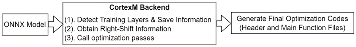
Figure 6: An overview diagram of the process of generating the optimization code in the CortexM backend. The numbers (1), (2), and (3) indicate the order implemented in the backend
First, the CortexM backend is compiled with an ONNX model as discussed in Section 2.2.3. This backend detects all layers (e.g., convolution, max-pooling, and ReLU layers) in the ONNX model and saves information about them, such as their names, strides, weights, dimensions, and pads. At the detection and compilation stages, the necessary parameters, such as input and output dimension, input and output channel, kernel size, stride, pad, weight, and bias in each layer are recorded in a list. Detecting all layers in a model ensures that all operators in the model are compiled and demonstrates the format compatibility between the operands in the model and operands in the CortexM backend. The operators and their parameters are changed according to the input models.
The second phase calls the optimization passes in the backend. It is used if any optimization pass is added to the pass manager of the backend. In addition, the backend creates a suitable weight format with operands in the CMSIS-NN library added in the cross-compilation process.
The third is the final optimization code generation phase for a device of the CortexM backend. The proposed CortexM backend creates all parameters in a model as well as related files such as Function-Call.cpp and pre-processing input data. However, the optimization is implemented on a few important phases including pre-processing input data, tuning the Pad parameter in the model, reducing the operator dimension, and tuning the final min function.
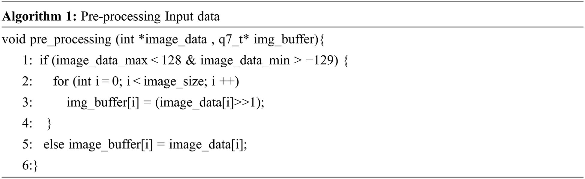
3.2.1 Pre-processing Input Data
Since the goal of building and optimizing the CortexM backend is to create a useful backend for the community, it is necessary to optimize the input data, which are mostly images. This process is not specific to ARM Cortex M devices and could be applied to image processing on other devices. An input image optimization pass is also included in the backend. Since the input data are loaded into the system in the form of an array of 8-bit integers, this array length will exceed the range (−129, 128) and overflow the memory. Therefore, it is necessary to develop a pre-processing function to map the image values to the range (−129, 128), as presented in Algorithm 1. Based on Algorithm 1, the input data array are shifted to the right in a round-robin manner until the array values are in the range (−129, 128) to save memory and to fit in the computation range of the CMSIS-NN library.
3.2.2 Tuning the Pad Parameter in Models
This section discusses the padding of ‘0’ values on the outside of an image so that the picture size matches the size of the kernel in the model. In ONNC, each layer is called an operator and its structure was already built in the ONNC compiler. Since there are many parameters in each layer of a model, which can affect the features of the input image, there is an important parameter called the Pad parameter in both the Convolution and MaxPooling layers. This parameter is used to calculate the feature range of the input images. If the parameters of the input images do not match the calculation range, then the kernel size is extended by supplementing the ‘0’ values into the margin edge for these images. This Pad value is the same as the auto Pad [15] value in the proposed model. Its computation is defined by two values called SAME_UPPER and SAME_LOWER. Based on those two values, the Pad parameter is optimized using Eqs. (4) and (5). Its main target is to produce an integer assemblage according to the floor() or ceil() function in the computation process of the model. In addition, supplementing the ‘0’ values into the margin edge of images makes the digits and image labels more prominent, which should improve recognition and classification. Based on Eqs. (4) and (5), the weight size of the model not only significantly decreases, but the computation speed for the application also increases, while barely affecting the original accuracy of the model due to the rounding margin of this function being very small.
where
3.2.3 Operator Dimension Reduction Techniques
This section discusses techniques to reduce the weight size of the addition and multiplication operators. In Section 3.1.2, the weights of the model were optimized by limiting their values to the range (−129, 128); however, at this point, they remain unsuitable for the new operators added in the CortexM backend. Because the CMSIS-NN library does not provide matrix addition and multiplication operators for 8-bit integers, these have been added to the backend to support matrix computation. Adding two new operators is also the reason for the memory overflow in the computation process. Therefore, to remedy the overflow while enabling matrix addition, matrix multiplication, and convolution layers, two new parameters have been added: two different Right-Shift values, (1)
Since the format of weights in ONNX (channel-height-width [CHW]) and the CMSIS-NN library (height-width-channel [HWC]) are different, the computation of matrix addition and matrix multiplication are problematic. As part of the proposed system, a function is designed and implemented to convert them into the HWC format. In this way, the ONNX model weight is converted to the HWC format so that it is compatible with the CMSIS-NN library. Additionally, the formats of the input weight (Matmul-Weight) of the matrix multiplication layer and the weight of the convolution layer are different. The conversion must be performed one more time. These conversions are included in the backend and are performed automatically when compiling it.
where
3.2.4 Tuning the Main Function
The main function is a final file that contains all computation layers of a model including all added optimization passes. The Cortex-M backend generates this main function and the detailed computation is shown in Algorithm 2. For each different model, this main function has different operators. The algorithm combines the input data pre-processing process with the detected layers to create a full main function containing all layers such as Convolution, Maxpooling, and ReLU. Algorithm 2 can be described in the following steps.
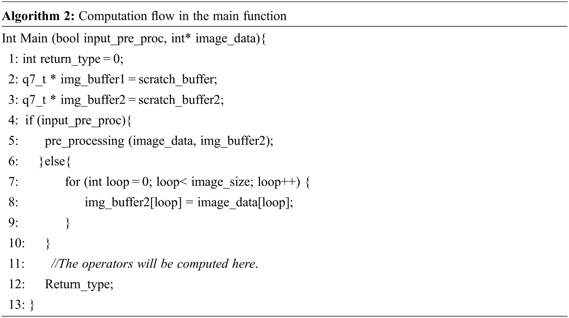
First, all header files and arrays are declared for the program. Second, the input image data pre-processing is performed depending on the input data. Finally, the program produces the result. All computations in this file are related to the CMSIS-NN library, which contains many convolution layers. Each layer requires different input parameters to perform different computations. Therefore, these functions are combined with the required parameters to generate a suitable main function, as shown in Algorithm 3.
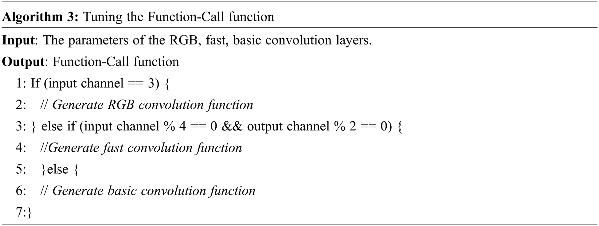
Its main function calls the proper convolution function based on the input channel. Since these convolution layers are limited by the input and output channels, these values are tuned to the main function. This algorithm only combines the computation of layers in the model with the pre-processing function; it does not affect the accuracy during the computation process. The arrays in the main function and the parameter values in the detected layers have different lengths after tuning. If the length is not fixed, many redundant ‘0’ elements exist in the output array, occupying a significant amount of memory. Therefore, these output parameters are adjusted by limiting the array size of the output variables to save memory. The formula to calculate the output file size is:
where
In the calculation process of the main function, two arrays are used to store the computation results as the input and output matrices. The input matrix is computed to obtain the output result and it becomes the input of the next layer. The final output matrix of the previous layer will become the input matrix of the next layer. Consequently, the memory is saved without allocating more matrices.
3.3 Featured Parameters of Applications
The final compilation result of the proposed backend with an ONNX model is to create a specific machine instruction for the target device. With ONNC, based on the specific applications, the user can redefine these featured parameters in their backend. This is an advantage of ONNC backends. In the approach employed in this paper, common source file types (i.e., *.cpp or *.h) are required, and these files are created. These file types are not only popular with users but also suitable for computations in the CMSIS-NN library. This also increases the inference speed in problems of recognition and image classification. With the proposed system, this phase is the most important because all features of a model are generated in it. Defining files, architectures of operands, and codes to generate these files are designed in the CortexM backend, and it can be extensible by adding or modifying any operands.
3.4 Application-Specific Phase
The application-specific phase uses the results of the previous phases to deploy an application-specific binary on the target device; on different devices, the implementation methods are also different. Therefore, to implement an application, the user must add some of the library and available applications to support the computation process. In this paper, the generated files are combined with the CMSIS-NN library and Mbed application to create a complete application. Mbed-CLI is an existing program used to compile related files into a single file. The Mbed-CLI program is installed with the command Embed-os-example-blinky [16] to create the Mbed CLI environment. Then, the Cross-compiler is used to combine the CMSIS-NN library and neural network kernels with all generated files by the backend to create the application file, called *.Bin file for the ARM Cortex-M devices. All the scripts are implemented by the command “mbed compile–t GCC_ARM–m target_device”, in which “mbed compile” calls the mbed compiler, and GCC_ARM calls the compiler tool for the ARM device. Finally, the *.Bin file is moved to the device to implement computation.
4.1 Hardware and Software Platform
The hardware platform used for these experiments was a Desktop-6TDMGP4 computer with an Intel Core i5-7500 processor and 8.00 GB RAM. The operating system was 64-bit Windows 10 and the programming language used was Visual C++. The Linux 16.04 LTS OS and tools were installed to compile the CortexM backend of the ONNC compiler. The experiments were performed on a NUMAKER_PFM_NUC472 device with 512 KB of flash memory and 64 KB of SRAM.
This section discusses the two experiments performed to assess the efficacy of the new backend: (1) handwritten digit recognition on the MNIST model and (2) image classification on the CIFAR-10 dataset with the AlexNet-Light model. The details of each model and dataset are introduced in Section 5. These two experiments were implemented separately. However, they have the same implementation diagram which is shown in Fig. 7.
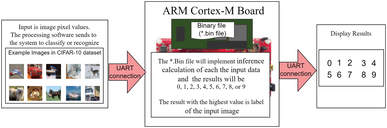
Figure 7: A diagram outlining the experiments to recognize the handwritten digits in the MNIST data and to predict the labels of images in the CIFAR-10 data
On the left of Fig. 7 is the input image of the system; these images are transmitted to the ARM board through software called Processing. In the middle is the ARM Cortex-M board containing the CortexM backend and the information of a model and its executive functions. On the right is the integer type’s output result because the handwritten digits and the labels of images are integer numbers. These parts are connected together by the UART port as a USB port. The selected models were first compiled with the ONNC compiler by the CortexM backend to create the *.Bin file for the experiment. Then the system was configured and a new window appeared along with a folder of the ARM board; this meant that the ARM Cortex device and PC were connected successfully. All tools and required programs must be put in the folder of the ARM Cortex-M device. After this, the processing software was started and the program was executed. At this time, a new window popped up to show that the Processing software and the system were connected successfully. The input data were sent from this software to the ARM board for computing. Finally, the results were displayed on the PC in a different new window.
5.1 Recognition of the MNIST Dataset
5.1.1 Dataset and Model Architecture
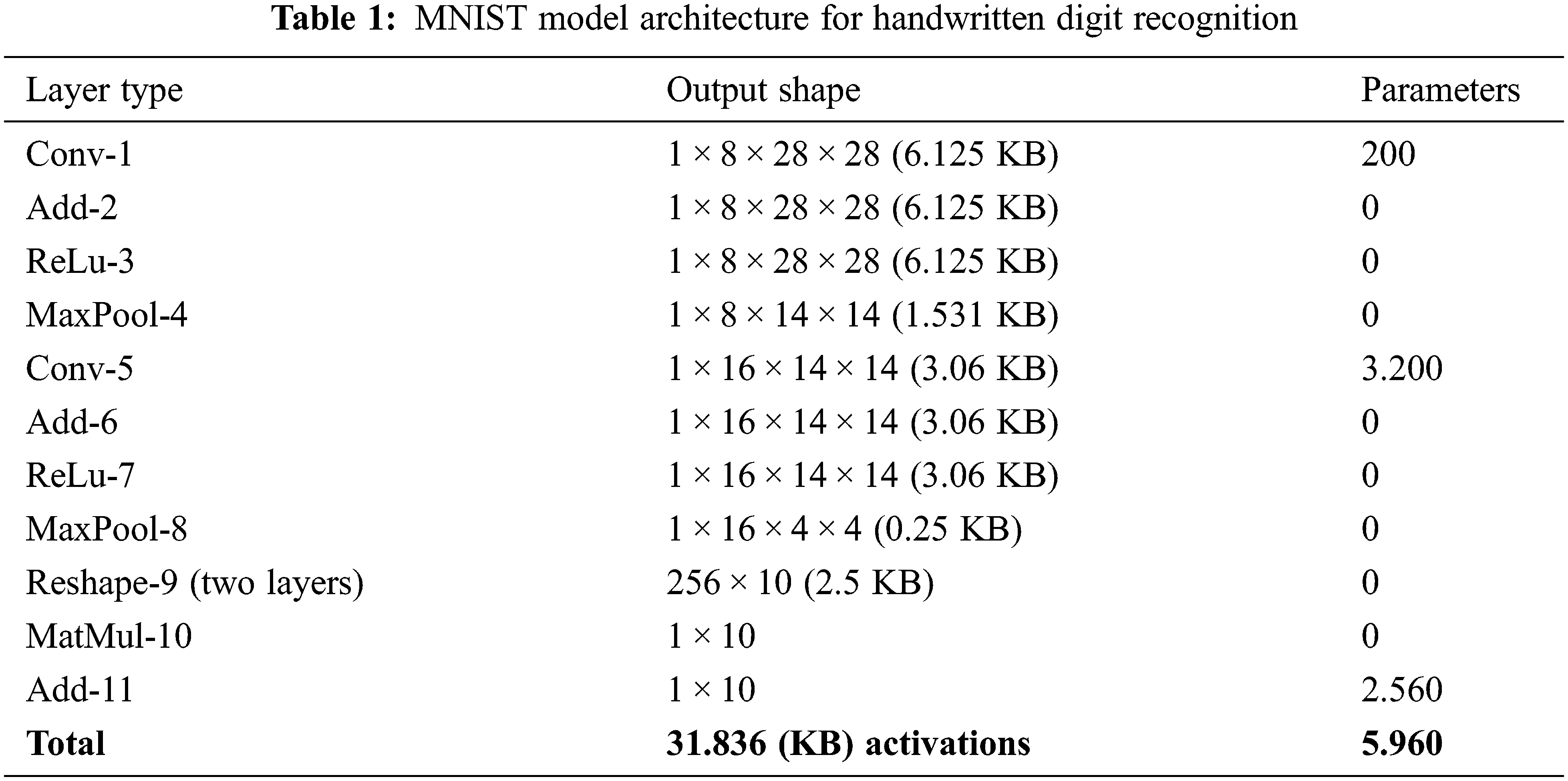
The MNIST [17] data and model were used for the first experiment and the model’s original structure and order of layers were kept. The detailed model architecture is shown as in Table 1. The input data were created by writing digits on the Processing software, and they were not trained with the MNIST model during the experiment so the validation data did not contain any information from the input data. The obtained result was the inference from validation data of the MNIST model.
The system was designed and developed for ARM Cortex-M devices with limited memory space and computation speed. Only one image sent from processing software was recognized each time. Due to the limited recognition speed of the system, the sample dataset of 1,500 images for each digit were created by many people with different writing styles and did not follow any particular rules, as shown in Fig. 8. They contained all edges of a digit written.
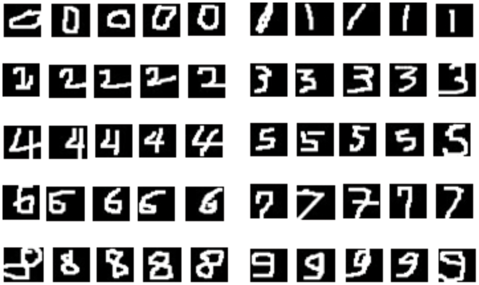
Figure 8: A sample image set of the handwritten digits, which was used to test the proposed backend
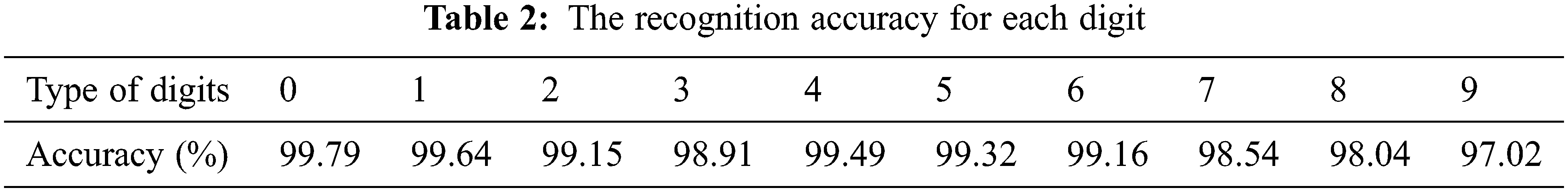
Digit recognition was implemented in the system using the sample image set shown in Fig. 8, and the results of recognizing each digit are shown in Table 2. The recognition accuracy was determined as follows: the handwritten digits were loaded into the system and the output was checked: if the output result showed the correct input digit then the recognition result was deemed correct. Digit recognition was conducted on different handwriting styles to give a more objective accuracy score. The average accuracy achieved was 98.90% across the various cases in the recognition process, including small and large digits, superimposed digits, and two digits written together. The results were impressive for a small device with limited memory.
The approach of this paper creates a CortexM backend for ONNC and implements the handwritten digit recognition with the MNIST model. When compared with some other state-of-art techniques it showed superior results for handwritten digit recognition, as shown in Table 3. All these studies used the same database and feature extraction method. The study in [18] used a convolution layer with 28 kernels/filter/patches and kernel sizes of 5 × 5 and 3 × 3 to extract the features. The neural network structure was deeply optimized and implemented in MATLAB 2018b. Their experiments were implemented on an NVIDIA 1060 GTX GPU device; their model size is also larger than the model size in this paper. Another study [19] used a deep learning model to recognize handwritten digits; however, it only obtained an accuracy of 96.63% with a larger and deeper network than in the present study. The studies in [20,21] implemented digit recognition on an embedded system. In both studies, the input digits were written on a whiteboard and transmitted to the board by a camera, but they only achieved accuracies of 98.23% and 98.00%, respectively. These models all needed to be trained with the MNIST model before implementing the experiment, which improved their accuracy. The model structures in [18–21] were more complex than in the present study; they used the convolutional neural network method and deep optimization of these networks after training with the MNIST dataset.
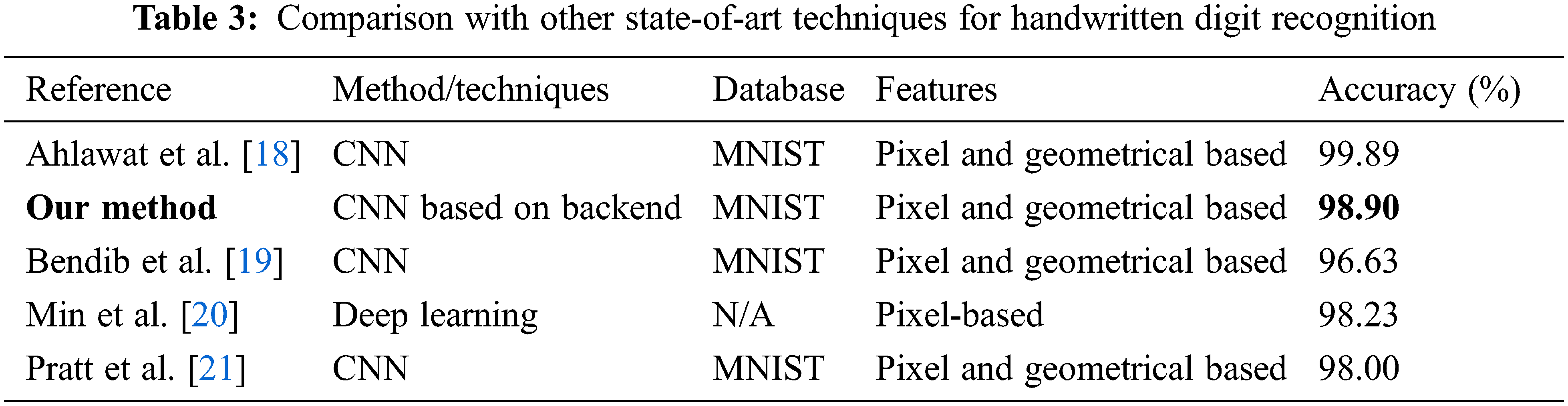
In contrast, the proposed system achieved a higher accuracy with a more straightforward structure. Some researchers used ensemble architectures for the same dataset to improve recognition accuracy, but the computational cost and testing complexity of these approaches were high because their databases had to be trained with the input data before implementing digit recognition. As a result, they achieved different accuracies for different ratios. The model size in these studies was larger than in the proposed model. Nevertheless, the accuracy of these models was not particularly high. In contrast, the approach of this paper achieved a recognition accuracy of 98.90% for the MNIST model without employing an ensemble architecture and without training on the input data.
In the experiment, it was found that the size and weight of the digits changed each time the input images were written or drawn using the computer mouse. Since these input images were not trained before the experiment, the validation dataset in the MNIST model did not contain any information about the input data. However, the accuracy of each digit after each recognition was almost consistent. It is clear that the difficulty in handwritten digit recognition is due to differences in writing styles and sizes. To overcome this difficulty, input images were created with different marker sizes and written styles to obtain more objective results in this experiment. In addition, whether the inference in the handwritten recognition system is true or not depends on the contrast of handwritten digits and the ambiguity of the digits in an image. If the images are less ambiguous, then the accuracy rises and vice versa. One of the typical ambiguities in the inference of handwritten digits is the similarity between digits. If digits are unclear or too similar to other digits, then the accuracy will be different.
During the experiment, it was discovered that some digits are easily confused even by the human eye. Fig. 9 shows that ‘1’ is very similar to ‘7’ while ‘4’ is very similar to ‘9’. This poses a significant challenge to researchers and developers in the development of handwriting recognition systems. It certainly affects the accuracy of these systems. Furthermore, inaccurate recognition can be caused by digits being written in unusual writing styles or sizes, handwriting mistakes, or the writing window being too small. In addition to the input data, the accuracy also depends on other factors such as the depth and the model’s weight due to quantization.
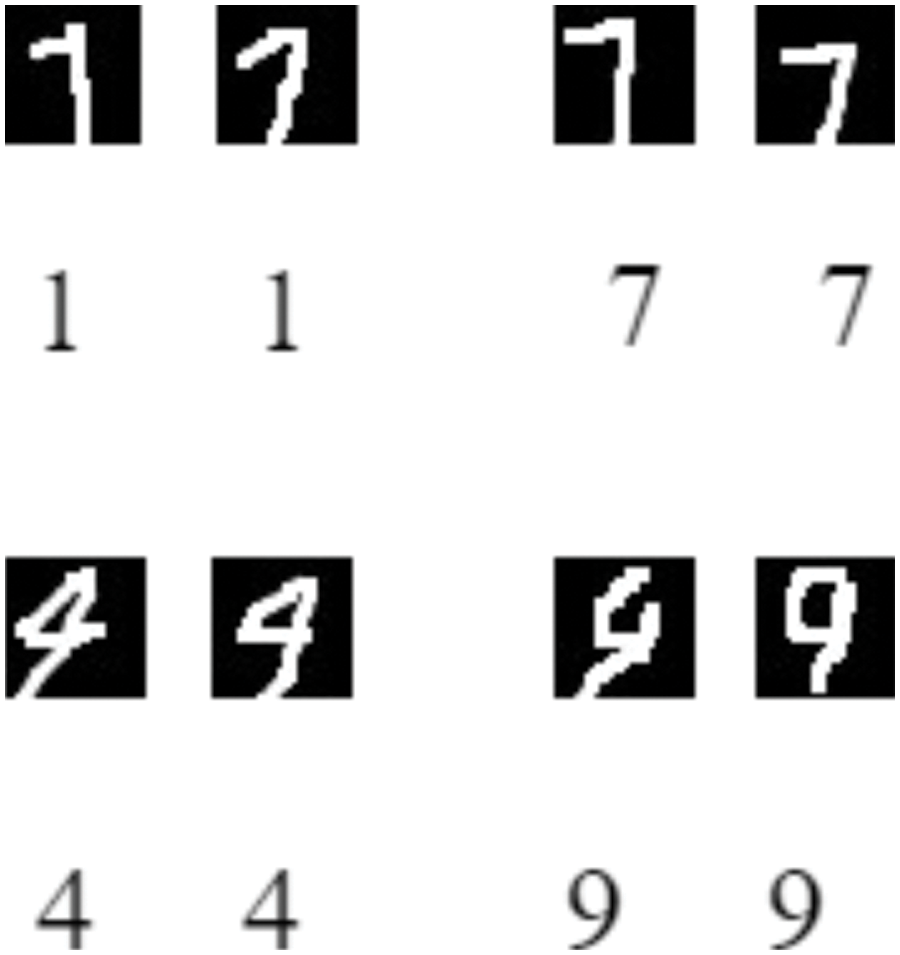
Figure 9: Examples of easily confused handwritten digits
5.2 Classification of the AlexNet-Light Model
5.2.1 Dataset and Architecture
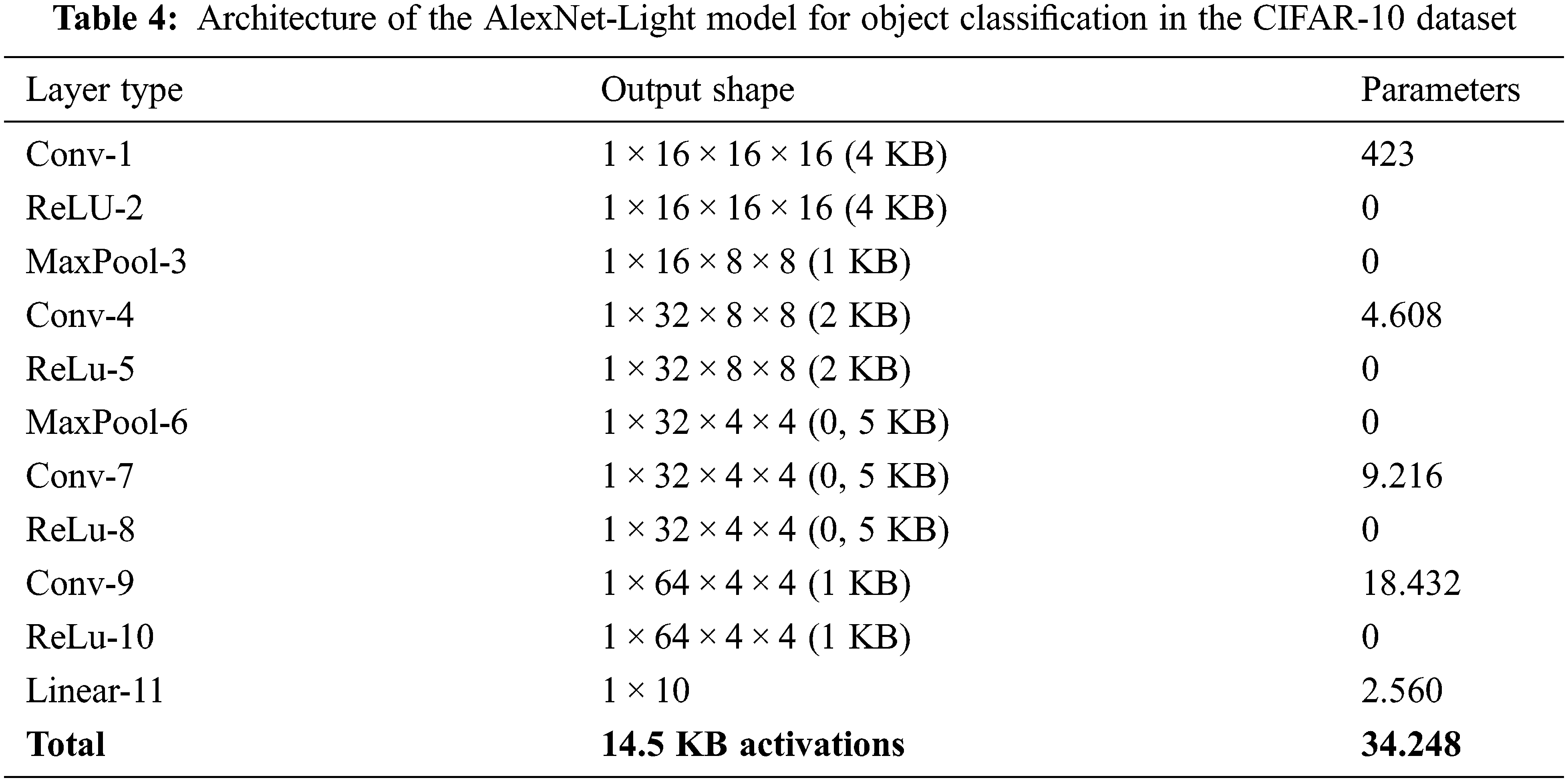
CIFAR-10 [22] is a well-known dataset for object classification with 60,000 natural RGB images, divided into a training set of 50,000 images and a testing set of 10,000 images. It comprises 10 classes of images: airplanes, automobiles, birds, cats, dogs, deer, horses, frogs, ships, and trucks. The AlexNet-Light model used for the second experiment was created based on the AlexNet [23] model and trained with the CIFAR-10 dataset. The architecture of the model is shown in Table 4.
In the CIFAR-10 dataset, each class is assigned a label and a corresponding integer, as listed in Table 5. The proposed system was used to classify the images according to these labels. Some sample images from the CIFAR-10 dataset and their corresponding labels are shown in Fig. 10.
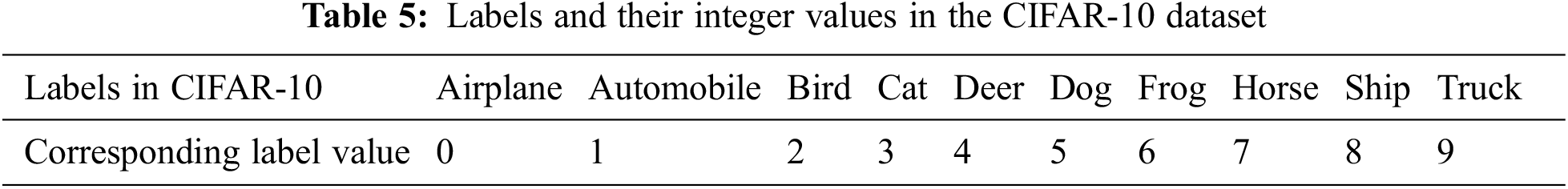
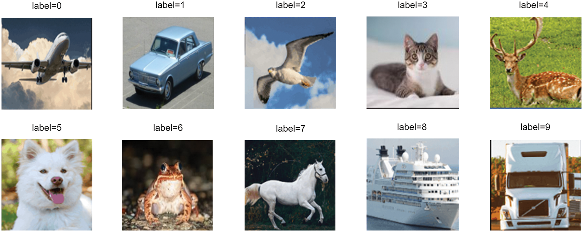
Figure 10: Example images and their corresponding labels in the CIFAR-10 dataset 1
The image classification diagram is shown in Fig. 7. Although the architecture was the same as in the previous experiment, the input data were replaced by the CIFAR-10 dataset. The *.Bin file contained the information of the AlexNet-Light model to perform classification. Random images were selected for each label to obtain objective results. The image classification accuracy was determined as follows: the input image for a given label (e.g., the Airplane label) was loaded and the output was checked. If the output showed the correct number (‘0’ in this case) then the classification result was deemed correct. The classification accuracy for each label is shown in Table 6—the overall accuracy was 90.55%.
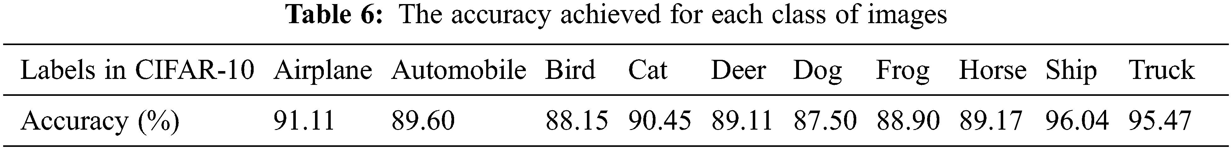
The image classification only took 0.58 ms, and it was straightforward to implement with limited memory. The architecture is ideal for use in embedded systems or small devices. Based on Table 6, the system achieved higher accuracy for the images labeled “Ship” and “Truck” than for “Dog”, “Bird”, and “Frog”. Note that the inference method predicted the output image using the pixel values. Therefore, if one image has many corresponding objects, then the prediction may be wrong. For example, if an image contains many objects similar to the background color, this “noise” will reduce the accuracy. That is a challenge in embedded systems because of their small memory.
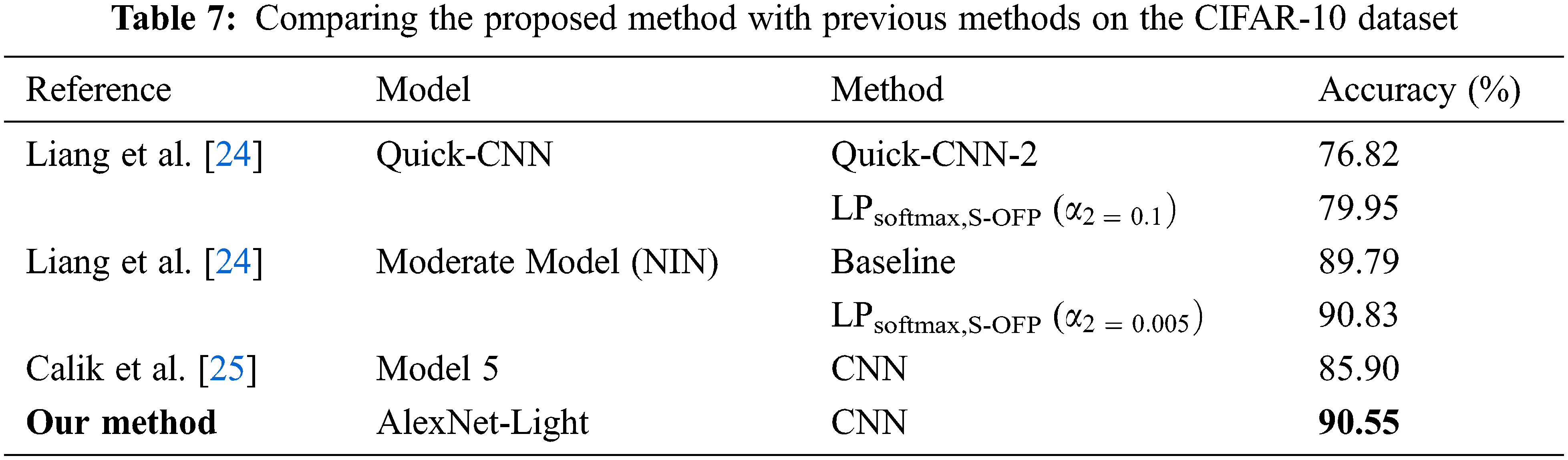
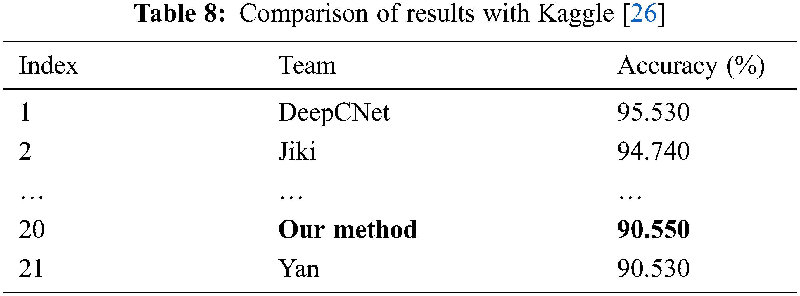
The model used was a small model with four convolution layers and one fully connected layer. Its accuracy was high when compared to other studies, as shown in Table 7. The result in [24] used the location property method of convolutional neural networks to classify images. This means that it had to find the optimal feature embedding location of the layer before the softmax operation. Its result had to be moved between the principal embedding direction and the secondary embedding direction before implementing classification. However, the accuracy was lower than the proposed system. In another branch of [24], the author used the optimization method in their model to classify the images. However, the model size was larger than in the proposed system, and their accuracy only achieved 85.90%. In the study [25], the models were challenging to implement for an embedded system due to memory overflow. It had three perceptron convolution multi-layers, and there was a three-layer perceptron within each multi-layer. Therefore, this model architecture is more complex than the model in this paper. In addition, some aspects of image classification used in popular methods such as feature extraction, adam, and dropout were taken into account in the proposed model. The results can be compared with another set of methods. Table 8 shows the accuracy compared with the work by Kaggle [26]. Although the accuracy achieved in this paper is not in the top 10 like that of Kaggle, it should improve with reduced label noise or a larger model structure. Furthermore, their models have a very complex model architecture with a large number of weights, making them infeasible for use in an embedded system. In contrast, the performance of the proposed system is higher for the classification system on small devices based on the pixel values of an input image.
This section discusses the proposed CortexM backend for the ONNC compiler by comparing it with other backends such as the C, NVIDIA Deep Learning Accelerator (NVDLA) [27], and LLVM backends. First, measured by the number of lines of source code, the proposed implementation is less complex than the others. Consequently, it is easier to port applications to it. Moreover, the proposed backend can save significant memory space and improve computational performance for target applications. The other approaches also generate more complicated code than the proposed system, especially when generating C++ code from an ONNX model. This complexity is mainly due to the efforts to maintain and increase the accuracy of the system after the compilation process. This is discussed in further detail in the following sub-sections. Because the memory of the target device is very small, applying auto transferring tools [28,29] to generate binary files may cause overflow. In addition, the operator structure of auto transferring tools is always fixed during compilation. In contrast, the proposed backend is more flexible and allows for the addition of operators into the binary file if necessary.
5.3.1 Implementation Complexity
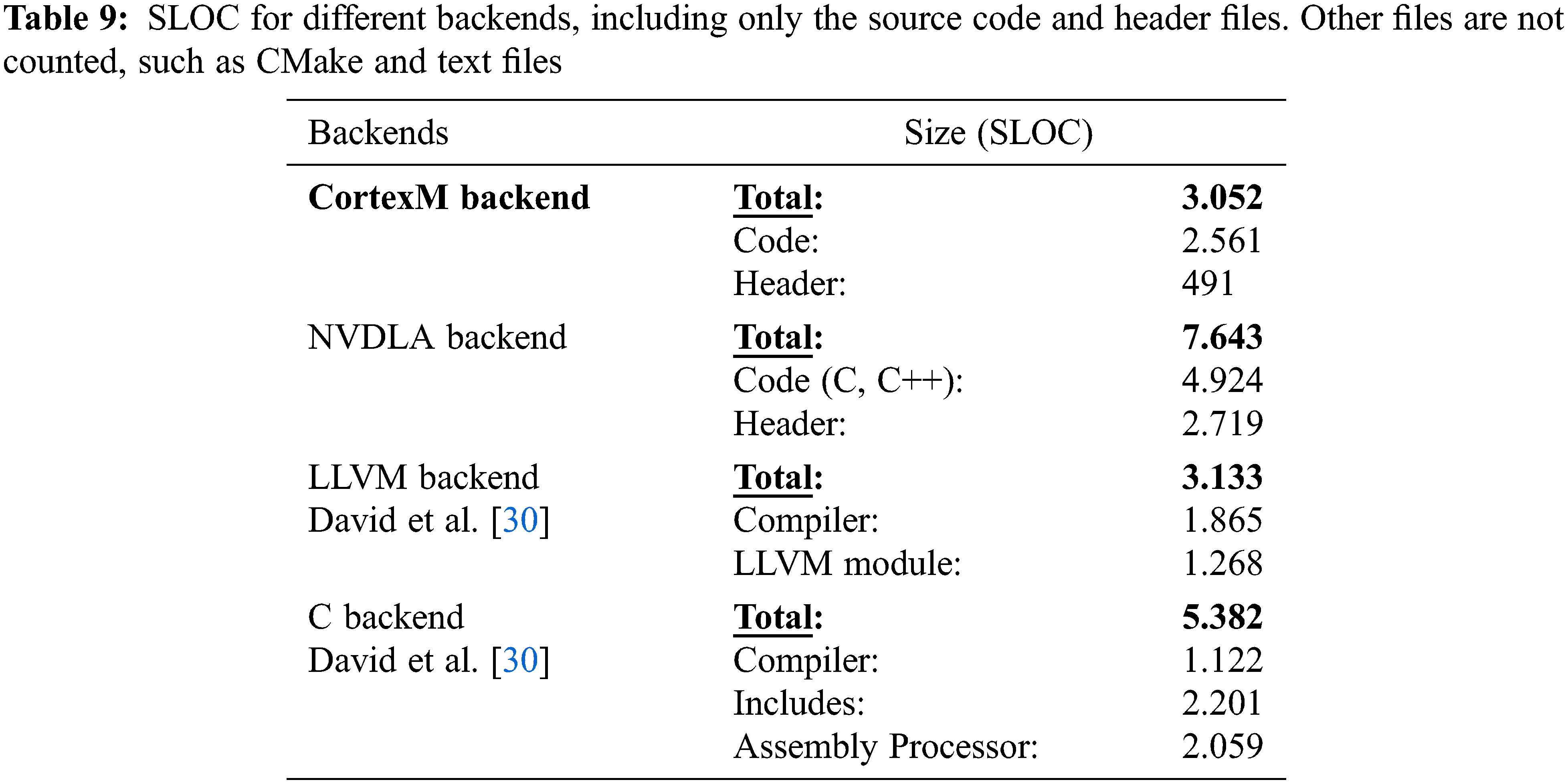
Implementation complexity is defined as the workload needed to implement a backend, including the build process, code generation, and extensibility. Each backend in ONNC can transform an instruction name into an opcode. When finishing the compilation process, it finds a suitable virtual memory space to store the operands. An ONNC backend consists of at least four phases (see Section 2.2.3). The proposed CortexM backend can be evaluated by comparing it with the NVDLA, C, and LLVM backends via the source lines of code (SLOC), as shown in Table 9. The code size of the CortexM backend is the smallest and that of the NVDLA backend is the largest when transforming opcodes into binary codes for the ARM Cortex-M device.
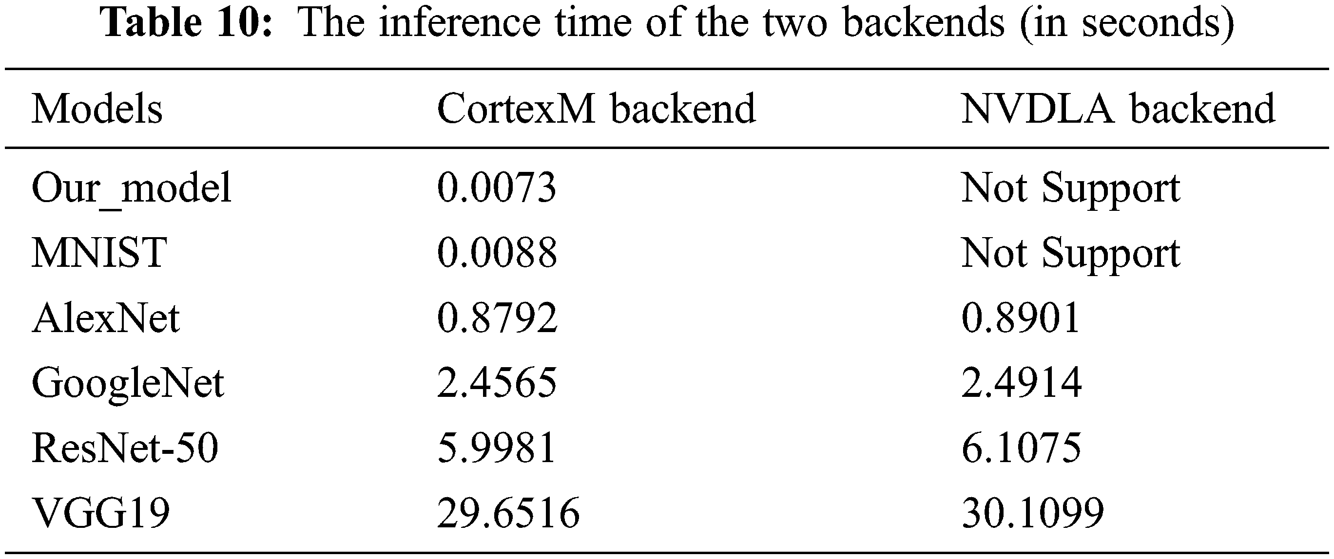
Both the C and LLVM backends are challenging to compile directly with these AI models. Therefore, the inference results can be affected by the conversion procedure between frameworks and backends. This section only compares the performance between the proposed backend and the NVDLA backend because they are all developed from the ONNC compiler with the same input data. To measure the performance, the total inference time was measured for some models with the benchmark tool [31] in ONNC. This benchmark tool only computes the compilation time of each layer in a model. The compilation time is obtained by reading the input operators of each layer to produce the output of all operators. The inference time of the two backends with the models is shown in Table 10. The inference time can change because each image has different weight values, so the overall compilation time of a model was measured for the two backends. Based on Table 10, the proposed backend is faster than the NVDLA backend by approximately 0.5% with the same weight and memory. The performance of the NVDLA backend is slower with larger memory than the proposed backend. In addition, since the structure of the NVDLA backend is different, many operators, such as matrix multiplication, are supported by the proposed backend but not by the NVDLA backend. For example, compiling the NVDLA backend with the MNIST model results in an “Unsupports MatMul” error. The user must add this operator in that backend and recompile the ONNC compiler to solve this problem.
A novel, highly efficient AI backend has been developed for the ONNC compiler for the ARM Cortex-M series, combined with a method to infer the performance of a target application. A backend helps the community to implement computations using an AI model on a target device. In the experiments on handwriting recognition on the MNIST dataset and image classification on the CIFAR-10 dataset, the proposed backend showed good accuracies of 98.90% and 90.55%, respectively, while the original accuracy of the MNIST and AlexNet models were 98.9% and 96.20%, respectively. These results show that the proposed system is not significantly less accurate than the original AI models. Furthermore, the performance of the new backend was evaluated by comparing it with the NVDLA, C, and LLVM backends to demonstrate that it is simpler and more efficient in terms of structure and code size. Although the proposed backend was developed for ARM Cortex-M devices, it can be applied to other boards and the ONNC compiler’s support. Users could deploy this backend widely on other small device series (e.g., the SMT32 and ARM Cortex-a devices) and mobile devices to validate the efficiency of the system. A docker image [32] is provided on GitHub for the research and development community.
Acknowledgement: We are grateful to the ARM equipment supplier called Nuvoton Electronics technology in Hong Kong and Skymizer Inc. in Taiwan to support the ONNC compiler.
Funding Statement: This work was supported in part by the Ministry of Science and Technology of Taiwan, R.O.C., the Grant Number of project 108-2218-E-194-007.
Conflicts of Interest: The authors declare that they have no conflicts of interest to report regarding the present study.
1Notice that the original resolution is 32 × 32. To show this image clearly for readers, we use a higher resolution one instead.
References
1. A. V. Aho, M. S. Lam, R. Sethi and J. D. Ullman, “Compilers: Principles, Techniques, and Tools,” in Computers & Technology, 2nd ed., vol. 1. New York: Addison-Wesley, ACM, pp. 1–1040, 2006. [Google Scholar]
2. M. Hall, D. Padua and K. Pingali, “Compiler research: The next 50 years,” Communications of the ACM, vol. 52, no. 2, pp. 60–67, 2009. [Google Scholar]
3. C. Lattner and V. Adve, “LLVM: A compilation framework for lifelong program analysis & transformation,” in Int. Conf. on Code Generation and Optimization (CoCGO), San Jose, CA, USA, IEEE, pp. 75–86, 2004. [Google Scholar]
4. T. Chen, T. Moreau, Z. Jiang, L. Zheng, E. Yan et al., “TVM: An automated end-to-end optimizing compiler for deep learning,” in 13th Int. Conf. on Symp. on Operating Systems Design and Implementation (CoSOSDI), USENIX, Carlsbad, CA, USA, no. 18, pp. 578–594, 2018. [Google Scholar]
5. J. Bai, F. Lu and K. Zhang, “Open neural network exchange (ONNX),” GitHub repository, 2019. [Online]. Available: https://github.com/onnx/onnx. [Google Scholar]
6. A. Аkanova and M. Kaldarova, “Impact of the compilation method on determining the accuracy of the error loss in neural network learning,” Technology Audit and Production Reserves, vol. 6, no.2, pp. 56, 2020. [Google Scholar]
7. G. J. Chaitin, “Register allocation and spilling via graph coloring,” Acm Sigplan Notices, vol. 39, no. 4, pp. 66–74, 2007. [Google Scholar]
8. S. Fang, W. Xu, Y. Chen and L. Eeckhout, “Practical iterative optimization for the data center,” ACM Transactions on Architecture and Code Optimization, vol. 12, no. 2, pp. 1–26, 2015. [Google Scholar]
9. A. H. Ashouri, G. Mariani, G. Palermo, E. Park, J. Cavazos et al., “Cobayn: Compiler autotuning framework using Bayesian networks,” ACM Transactions on Architecture and Code Optimization (TACO), vol. 13, no. 2, pp. 1–25, 2016. [Google Scholar]
10. M. Tewary, Z. Salcic, M. B. Abhari and A. Malik, “Compiler-assisted energy reduction of java real-time programs,” Microprocessors and Microsystems, vol. 89, pp. 104436, 2022. [Google Scholar]
11. S. N. Agathos, V. V. Dimakopoulos and I. K. Kasmeridis, “Compiler-assisted, adaptive runtime system for the support of OpenMP in embedded multicores,” Parallel Computing, vol. 110, pp. 102895, 2022. [Google Scholar]
12. R., Anchu and V. K. Nandivada, “DisGCo: A compiler for distributed graph analytics,” ACM Transactions on Architecture and Code Optimization (TACO), vol. 17, no. 4, pp. 1–26, 2020. [Google Scholar]
13. W. Lin, W. Fen, D. Y. Tsai, L. Tang, C. T. Hsieh et al., “ONNC: A compilation framework connecting ONNX to proprietary deep learning accelerators,” in Int. Conf. on Artificial Intelligence Circuits and Systems (CoAICAS), Hsinchu, Taiwan, IEEE, pp. 214–218, 2019. [Google Scholar]
14. L. Lai, N. Suda and V. Chandra, “CMSIS-NN: Efficient neural network kernels for Arm cortex-M CPUs,” Neural and Evolutionary Computing, vol. 1, no. 1, pp. 1–10, 2018. [Google Scholar]
15. G. Ramalingam, “Pad,” GitHub repository, 2018. [Online]. Available: https://github.com/onnx/onnx/blob/rel-1.3.0/docs/Operators.md#Pad. [Google Scholar]
16. A. Bridge, M. Kojtal, S. Grove, C. Monrreal, E. Donnaes et al., “Embed-os-example-blinky,” GitHub repository, 2020. [Online]. Available: https://github.com/ARMmbed/mbed-os-example-blinky. [Google Scholar]
17. Y. LeCun, C. Cortes and C. J. Burges, “MNIST handwritten digit database,” ATT Labs, pp. 2, 2010. [Online]. Available: http://yann.lecun.com/exdb/mnist. [Google Scholar]
18. S. Ahlawat, A. Choudhary, A. Nayyar, S. Singh and B. Yoon, “Improved handwritten digit recognition using convolutional neural networks (CNN),” Sensors, vol. 20, no. 12, pp. 3344, 2020. [Google Scholar]
19. I. Bendib, A. Gattal and G. Marouane, “Handwritten digit recognition using deep CNN,” in 1st Int. Conf. on Intelligent Systems and Pattern Recognition (CoISPR), ACM, New York, NY, United States, pp. 67–70, 2020. [Google Scholar]
20. J. H. Min, N. D. Vinh and J. W. Jeon, “Real-time multi-digit recognition system using deep learning on an embedded system,” in 12th Int. Conf. on Ubiquitous Information Management and Communication (CoUIMC), ACM, Langkawi, Malaysia, no. 17, pp. 1–6, 2018. [Google Scholar]
21. S. Pratt, A. Ochoa, M. Yadav, A. Sheta and M. Eldefrawy, “Handwritten digits recognition using convolution neural networks,” Journal of Computing Sciences in Colleges, vol. 34, no. 5, pp. 40–46, 2019. [Google Scholar]
22. B. Recht, R. Roelofs, L. Schmidt and V. Shankar, “Do CIFAR-10 classifiers generalize to CIFAR-10?,” Machine Learning, IEEE, vol. 1, no. 1, pp. 1–25, 2018. [Google Scholar]
23. A. Krizhevsky, I. Sutskever and G. E. Hinton, “Imagenet classification with deep convolutional neural networks,” Communications of the ACM, vol. 60, no. 6, pp. 84–90, 2017. [Google Scholar]
24. C. Liang, H. Zhang, D. Yuan and M. Zhang, “Location property of convolutional neural networks for image classification,” IEEE Transactions on Neural Networks and Learning Systems, vol. 32, no. 9, pp. 3831–3845, 2020. [Google Scholar]
25. R. C. Calik and M. F. Demirci, “Cifar-10 image classification with convolutional neural networks for embedded systems,” in 15th Int. Conf. on Computer Systems and Applications (CoCSA), Aqaba, Jordan, IEEE, pp. 1–2, 2019. [Google Scholar]
26. B. Graham, A. Thomas, F. Sharp, P. Culliton, D. Nouri et al., “Kaggle competition,” Kaggle, 2018. [Online]. Available: https://www.kaggle.com/c/cifar-10/leaderboard. [Google Scholar]
27. W. Lin, W. Fen, C. T. Hsieh and C. Y. Chou, “ONNC-based software development platform for configurable NVDLA designs,” in Int. Conf. on VLSI Design, Automation and Test (CoVLSI-DAT), Hsinchu, Taiwan, IEEE, pp. 1–2, 2019. [Google Scholar]
28. D. Smirnov, G. Wang, D. Robinson, P. Sharma, C. Sun et al., “ONNX runtime,” GitHub repository, 2021, [Online]. Available: https://www.onnxruntime.ai. [Google Scholar]
29. M. Abadi, A. Agarwal, P. Barham, E. Brevdo, P. Chen et al., “Tensorflow: A system for large-scale machine learning,” in 12th USENIX Symp. on Operating Systems Design and Implementation, (OSDI), USENIX, Savannah, GA, USA, vol. 1, no. 1, pp. 265–283, 2018. [Google Scholar]
30. T. David and M. M. T. Chakravarty, “An LLVM backend for GHC,” in 3rd Int. Conf. on ACM Haskell Symp. on Haskell (HSH), ACM, Baltimore, Maryland, USA, pp. 109–120, 2010. [Google Scholar]
31. P. Y. Chen, “ONNC-Utilities,” GitHub repository, 2019. [Online]. Available: https://github.com/ONNC/onnc/blob/master/docs/ONNC-Utilities.md. [Google Scholar]
32. C. T. Hsieh, “ONNC community edition,” GitHub repository, 2020. [Online]. Available: https://github.com/ONNC/onnc-tutorial/blob/master/lab_2_Digit_Recognition_with_ARM_CortexM/lab_2.md. [Google Scholar]
Cite This Article
 Copyright © 2023 The Author(s). Published by Tech Science Press.
This work is licensed under a Creative Commons Attribution 4.0 International License , which permits unrestricted use, distribution, and reproduction in any medium, provided the original work is properly cited.
 Downloads
 Citation Tools