Aquila Optimization with Machine Learning-Based Anomaly Detection Technique in Cyber-Physical Systems

1  Introduction

Cyber physical system (CPS) involves incorporating the physical system into the real-time and control software in the cyber world, whereby the network interconnects the two worlds and is accountable for the data exchange amongst themselves [1]. Wide-ranging development in communication technology might assist real-time communication with lower latency making them possible to remotely control various physical systems and provide smart facilities to CPS users [2]. Furthermore, adapting wired and wireless networks in a CPS allows the state of a large number of industrial equipment to be observed. Consequently, it is the potential to flexibly organize and handle a complicated industrial system [3]. Therefore, the CPS is the fundamental technology for different industrial sectors involving smart grid systems, smart transportation systems, and medical systems. Fig. 1 displays the overview of CPS.

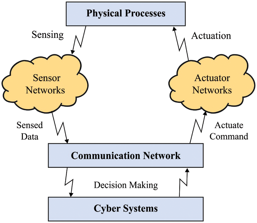
Figure 1: Overview of CPS

As the connectivity of CPS rises and becomes increasingly sophisticated, the path through which attackers infiltrate the CPS is growing [4]. The network that connects the CPS and the control software is particularly susceptible to an external attacker that aims to invade the physical system and cause a malfunction in the CPS [5]. Once the attacker access the network, the control authority of CPS operation on the network can be seized, the implementation of control critical software is disturbed in the cyber world, and the attacker's power of the CPS or control the physical system with a deceitful attack detection technique [6]. The CPS attack harms industrial processes and equipment, which causes human casualties and economic losses. To identify unexpected errors and attacks in CPS, an anomaly detection system is introduced to mitigate the threat [7]. For instance, statistical models (for example, Gaussian model, histogram-based model) based method, rule, and state estimation (for example, Kalman filter) are exploited to learn the typical status of CPS. But the method usually needs expert knowledge (for example, the operator manually extracts some rules) or should be aware of the fundamental distribution of standard datasets [8].

Machine learning (ML) approaches don’t depend on domain-specific knowledge. However, they typically need a massive amount of labelled datasets (for example, classification-based method). They also could not capture the unique attribute of CPS (for example, spatiotemporal relationship). An intrusion detection system (IDS) ensures network transmission security [9]. Physical property is captured to represent the immutable nature of CPS. Program implementation semantics are considered to protect the control system. But, as CPS becomes more complex and the attack is more stealthy, this method is more difficult to ensure the status of CPS (for example, protecting multi-variate physical measurement). It requires further domain knowledge (for example, correlation and more components) [10]. An anomaly detection system needs to adapt to capture novel features of CPS.

This article develops an Aquila Optimizer with Parameter Tuned Machine Learning Based Anomaly Detection (AOPTML-AD) technique in the CPS environment. The presented AOPTML-AD model pre-processes the network data by converting it into a compatible format. In addition, the improved Aquila optimization algorithm-based feature selection (IAOA-FS) technique is designed to choose an optimal feature subset. Furthermore, the chimp optimization algorithm (ChOA) with an adaptive neuro-fuzzy inference system (ANFIS) model can be employed to recognise anomalies in the CPS environment. The ChOA is applied for optimal adjustment of the membership function (MF) indulged in the ANFIS model. The performance validation of the AOPTML-AD algorithm is carried out using the benchmark datasets.

2  Related Works

Thiruloga et al. [11] introduce a new unsupervised technique for detecting cyber-attacks in (CPS). The authors define an unsupervised learning method by using a Recurrent Neural network (RNN) that can be a time sequence predictor in this method. They employ the Cumulative Sum technique for identifying anomalies in a replication of a water treatment plant. The presented technique not just identifies anomalies in the CPS but also detects a sensor that has been attacked. In [12], the researchers review the existing deep learning (DL)-related anomaly detection (DLAD) techniques in CPSs. They suggest a taxonomy relating to the anomaly’s types, implementation, evaluation metrics, and strategies for understanding the necessary properties of existing techniques. Additionally, they use this taxonomy for identifying and highlighting novel features and models in every CPS field. Luo et al. [13] suggest an anomaly detection method by integrating the intellectual DL method called convolutional neural network (CNN) with Kalman Filter (KF) related Gaussian-Mixture Model (GMM). The suggested method can be utilized to detect abnormal conduct in CPSs. This recommended structure has 2 significant procedures. The primary step was pre-processing the data by filtering and transforming the original data into an innovative format and attained privacy data preservation. And then, the research scholars suggested the GMM-KF integrated deep CNN method for anomaly detection (AD) and precisely assessed the posterior probability of legitimate and anomalous events in CPSs.

Nagarajan et al. [14] suggested the Data-Correlation-Aware Unsupervised DL method for AD in CPS that utilizes an undigraph framework for storing samples and implied relation amongst samples. The authors devise a dual-AE for training both original features and implied correlation features amongst data. They build an estimation network by use of GMM for evaluating the probability sample distribution for the completion of an anomaly analysis. Xi et al. [15] recommend a new time sequence anomaly detection technique termed Neural System Identification and Bayesian Filtering (NSIBF), where a specially crafted NN framework was posed for system identification. Singh and Feng et al. [16] offer a structure and method to develop a cyber-physical AD system (CPADS) that uses synchrophasor dimensions and network packet properties to detect data integrity and transmission failure assaults on measurement and control signals in CRAS. The suggested ML-related method adopts a rules-related technique for selecting relevant input features, uses DT and variational mode decomposition (VMD) methods for developing multiple classification methods, and executes final event identification utilizing a rules-related decision logic. In [17], an intelligent anomaly identification (IAI) method for these mechanisms was provided using data-driven tools which leverage a multi-class support vector machine (MSVM) for anomaly localization and classification. The impacts of cyber-anomalies like false data injection and denial of service (DoS) assaults that target the transmission network were taken in this study.

3  The Proposed Model

In this study, a new AOPTML-AD model intends to recognize and detect anomalous behaviour in the CPS environment. The presented AOPTML-AD framework initially pre-processed the network data by converting them into a compatible format. The IAOA-FS method is designed to elect an optimal subset of features. This study utilises the ChOA with the ANFIS model for anomaly detection and classification. Fig. 2 depicts the overall process of the AOPTML-AD approach.

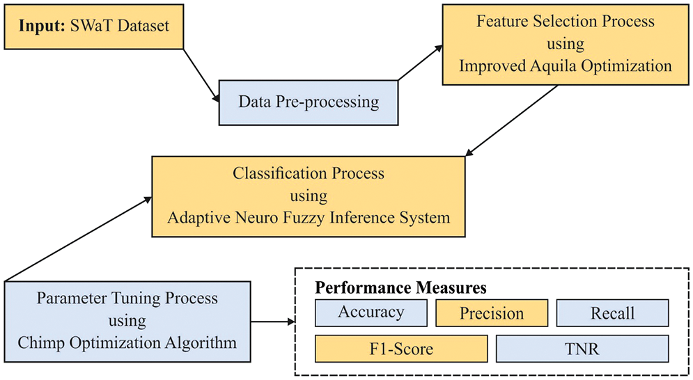
Figure 2: Overall process of AOPTML-AD approach

3.1 Data Pre-processing

The presented AOPTML-AD framework initially pre-processed the network data by converting them into a compatible format. The data accumulated in real applications is noisy and consist of certain missing values or errors. Moreover, the scale of data from various kinds of sensors could differ. Thus, data cleaning becomes essential and significant for further processing. The z -score normalization can be utilized to normalize the data. Thus, the data which is collected contain unit variance and zero means. The normalization is attained by making use of the equation, which is given below.

xi′=xi−μiσi                                  (1)

Here, xi′ was the normalized data. xi is measurement data from the i-th sensor. μi refers to the mean value of the measurement. σi denotes the standard deviation.

3.2 Design of IAOA-FS Model

Once the input data is pre-processed, the IAOA-FS algorithm is designed to choose an optimal subset feature. AOA was recently introduced. It was claimed and proven with better performance and faster convergence speed than other techniques [18]. Also, the individual in a swarm of the AOA has four ways to upgrade its location, but they could only select two during the first 2/3 full process in exploration and two during the exploitation process. In the presented technique, there exist four approaches for individuals as follows:

Strategy 1: Expanded exploration.

Xi(t+1)=Xbest(t)×(1−tT)+XM(t)−Xbest(t)∗r1            (2)

In Eq. (2), Xi(t+1), Xbest(t), and XM(t) represent the location of i−th individuals at t+1 iteration, the best position at the existing iteration, and a mean position of each individual at a current iteration correspondingly. XM(t) is evaluated by using the following expression:

XM(t)=1N∑i=1N⁡Xi(t)                                                                  (3)

In Eq. (3), Xi(t) refers to the location of i−th individuals at t iterations. N denotes the number of individuals in swarms. r1 represents the arbitrary value in Gaussian distribution with the range of zero and one.

Strategy 2: Narrowed exploration.

Xi(t+1)=Xbest(t)×Leνy(D)+XR(t)+(y−x)∗r2                        (4)

In Eq. (4), Leνy(D) denotes the Levy flight in the following formula:

Levy(D)=s×μ×σ|v|1β                                            (5)

where s=0.01 was a constant variable, r2 was the alternative random number. μ, v denotes random numbers between [0, 1]. The following expression evaluates σ:

σ=Γ(1+β)× sin (πβ2)Γ(1+β2)×β×2β−12                                             (6)

where β=1.5 was a constant value. XR(t) indicates a randomly chosen candidate at the current iteration. y and x indicate the spiral shape:

y=r× cos (θ)                                                                 (7)

x=r×sin (θ)                                                                   (8)

r=r1+U×D1                                                                    (9)

θ=−ω×D1+θ1                                                              (10)

θ1=3π2                                                                    (11)

From the expression, r1 represents a fixed number within [1, 2]. D1 represents the integer numbers from 1 to the length of problems. ω=0.005 indicates a fixed constant number.

Strategy 3: Expanded exploitation.

Xi(t+1)=α×[Xbest(t)−XM(t)+δ×[(UB−LB)×r3+LB]                  (12)

In Eq. (12), [LB, UB] represents the definitional domain of the provided problem. α and δ denote 2 fixed smaller numbers. r3 refers to the third random number in the Gaussian distribution.

Strategy 4: Narrowed exploitation.

Xi(t+1)=QF×Xbest(T)−G1×Xi(T)×r4−G2×Leνy(D)+r5×G1         (13)

In Eq. (13), QF indicates the quality function utilized to equilibrium the searching technique and is evaluated by the following formula:

QF(t)=T2×τ6−1(1−T)2                                                     (14)

G1=2r7−1                                                               (15)

G2=2×(1−τT)                                                               (16)

r4, r5,r6, and r7 denote the fourth to seventh random numbers.

The IAOA is derived by including the quasi-oppositional based learning (QOBL) concept. In the AOA, the population tries to reach the optimal solutions located in an identified place. Thus, the water strider attempts to go to the same places, so the diversity of individuals is lost. A familiar process amongst the meta-heuristics is utilizing the Quasi Opposition-Based Learning (QOBL) approach to resolve this problem. It is executed as follows:

Xij(t)={αj+(αj−Xij(t))×β if(Xij(t)<αj)αj−(Xij(t)−αj)×β if(Xij(t)≥αj)                                (17)

i∈[1, I],j∈[1,J],k∈[1, K]                                                    (18)

αj=12×(X¯+X_)                                                          (19)

Whereas yijm describes the jth count of ith quasi-opposition solution at kth iteration, J refers to the variables number, β implies the arbitrary amount from the range of zero and one, and X_ and X¯ signify the minimal and maximal of a jth variable.

The fitness function (FF) of the IAOA-FS technique is developed to have a balance between the classification accuracy (maximum) and the number of selected features in every solution (minimum) attained by utilizing this selected feature, Eq. (20) denotes the FF to estimate solution.

Fitness=αγR(D)+β|R||C|                                               (20)

From the expression, γR(D) refers to the K-nearest neighbour (KNN) classification’s classification error rate. |R|  exhibits the cardinality of the selected subset, and |C| shows the overall number of features in the data, α, and β indicate two variables equivalent to the significance of subset length and classification quality. ∈ [1, 0] and β=1−α.

3.3 ANFIS Classification

At this stage, the chosen features are passed into the ANFIS model and are utilized for the recognition of anomalies in the CPS environment. Generally, ANFIS produces a mapping among outputs and inputs by applying “IF-THEN rules” (otherwise called as “Takagi-Sugeno inference model”) [19]. As shown, the input of Layer 1 is characterized as x and y , whereby the output of the ith node is signified as O1i , as follows:

O1i=μAi(x), i=1,2, O1i=μBi−2(y), i=3,4                            (21)

μ(x)=e−(x−ρiαi)2,                                                    (22)

From the expression, μ refers to the generalized Gaussian membership function. The membership value of μ is characterized as Ai and Bi . The premise parameter set is characterized as αi and ρi . Furthermore, Eq. (23) determines the output of Layer 2:

O2i=μAi(x)×μBi−2(y)                                                         (23)

Eq. (24) describes the output of Layer 3:

O3i=w¯i=ωiΣ(i=1)2ωi,                                                 (24)

In Eq. (24), wi represents the i - th  node output from the preceding layer.

The output of Layer 4 is characterized as follows:

O4,i=w¯ifi=w¯i(pix+qiy+ri)                                             (25)

In Eq. (25), f represents a function that integrates the input and parameter of the network. The resulting parameter of node i is denoted as ri, qi , and pi.

At last, the output of Layer 5 is characterized as follows:

O5=∑i⁡w¯i fi (26)

3.4 Parameter Tuning Using ChOA

At the final stage, the ChOA is applied for optimal adjustment of the membership function (MF) involved in the ANFIS method. The ChoA is inspired by chimps’ social status relationship and hunting behaviour. The four individual groups searched the problem space locally and globally, utilizing its unique pattern [20]. The drive and chase are provided as the subsequent formulas.

d=|c.xprey(t)−m.xchimp(t)|                                       (27)

xchimp(t+1)=xprey(t)−a.d                                 (28)

The present iteration number was determined with the symbol t , and a , m , and c were the co-efficient vectors, xprey signifies the prey vector place, and xchimp provides the chimp vector place. a , m , and c are demonstrated by the calculation that follows.

a=2.f.a1−f                                                         (29)

c=2.r2                                                            (30)

m=Choatic−value                                                       (31)

The nonlinear reduction of f was completed, from 2.5 to , in both stages. The arbitrary vectors were created from all the iterations, 2 arbitrary sets were allocated to r1 and r2 , and the m value was created in several chaotic maps.

During the exploitation stage, the chimp’s performance was modelled by formulas as follows.

dattacker=|c1.xattacker−m1.x|                                 (32)

dbarrierr=|c2.xbarrier−m2.x|                                  (33)

dchaser=|c3.xchaser−m3.x|                                     (34)

ddriver=|c4.xdriver−m4.x|                                     (35)

x1=xattacker − dattacker.a1                                  (36)

x2=xbarrier−dbarrier.a2                                      (37)

x3=xchaser−dchaser.a3                                         (38)

x4=xdriver−ddriver.a4                                          (39)

x(t+1)=x1+x2+x3+x44                                       (40)

xchimp(t+1)={xprey(t)−a.difμ<0.5Chaotic−valueifμ≥0.5             (41)

In the above formulas, c implies the arbitrary vector range from zero to two (i.e., [O,2] ), and a refers to the arbitrary variable range in [−2f, 2f]. During this case, the chaotic map, a primary value, is fixed to 0.7 from image thresholding optimized problems.

The original ChOA technique integrates 6 distinct chaos maps and 2 distinct sets of formulas for upgrading dynamic approaches. The dynamic model was utilized to define the coefficients c1, c2, c3 , and c4.

For the simplicity of this work, only one group of dynamic models and one chaos map are utilized. The chaos map was recognized as Gauss or Mouse. It can be determined as:

xi+1={1xi=01mod(xi,1)otherwise                            (42)

During the final phase, chimps relinquish their hunting responsibility and then obtain meet and succeeding social drive (sex and grooming). It can strive to gather meat chaotically during the outcome. For great dimensional problems, ChOA is developed to address two problems of slow convergence speed and traps from local optima. This chaotic performance in the final step supports chimps in overcoming the two problems of entrapment in local optimum and sluggish convergence rate from higher dimension problems resolving.

The ChoA method extracts the fitness function (FF) to obtain improvised classifier outcomes. It fixes a positive integer to denote the superior performance of the candidate solutions. In this work, the reduction of the classifier error rate can be regarded as the FF, as presented below in Eq. (43). The optimum solution comprises a minimum error rate, and the poor solution receives a higher error rate.

fitness(xi)=ClassifierErrorRate(xi)=number of misclassified samples total number of samples∗100 (43)

4  Results and Discussion

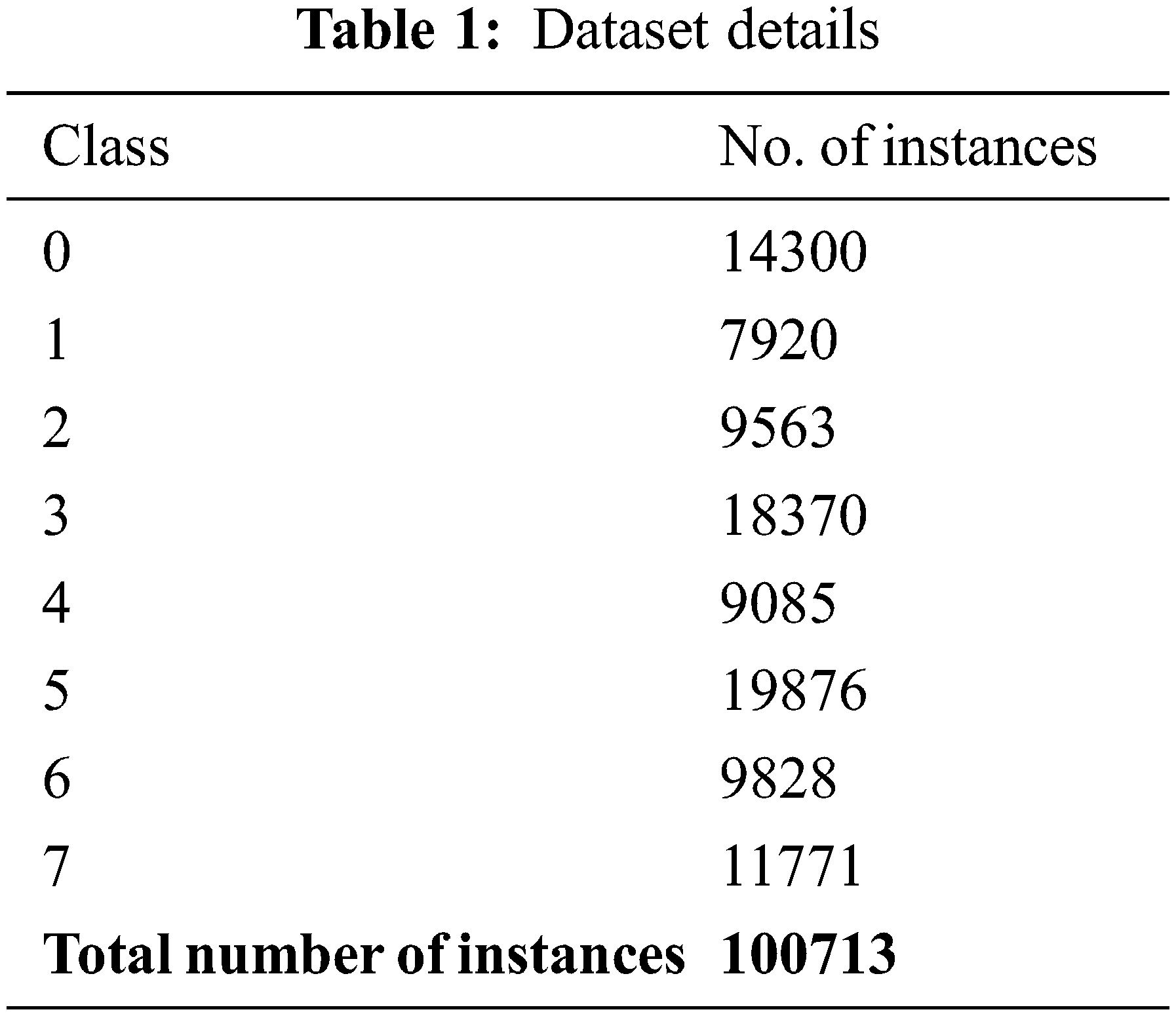
The experimental validation of the presented model is tested using the SWaT dataset [21]. It offers real data from a simpler form of the real-world water treatment plant. The datasets enable authors to devise and evaluate defence mechanisms for CPSs and comprise both network traffic as well as data concerning the physical property of a system. The dataset holds 100713 samples with seven class labels, as depicted in Table 1.

The confusion matrices generated by the AOPTML-AD model on distinct training (TR) and testing (TS) datasets are shown in Fig. 3. On 70% of TR data, the AOPTML-AD model has identified 9695 samples into class0, 5354 samples into class1, 6476 samples into class2, 12598 samples into class3, 6158 samples into class4, 13512 samples into class5, 6628 samples into class6, and 7974 samples into class 7. Also, on 30% of TS data, the AOPTML-AD method has identified 4241 samples into class 0, 2266 samples into class1, 2807 samples into class2, 5475 samples into class3, 2582 samples into class4, 5748 samples into class5, 2880 samples into class6, and 3363 samples into class7. In addition, on 80% of TR data, the AOPTML-AD technique has identified 11122 samples into class 0, 6164 samples into class 1, 7405 samples into class2, 14449 samples into class3, 7142 samples into class4, 15561 samples into class5, 7462 samples into class6, and 9164 samples into class7.

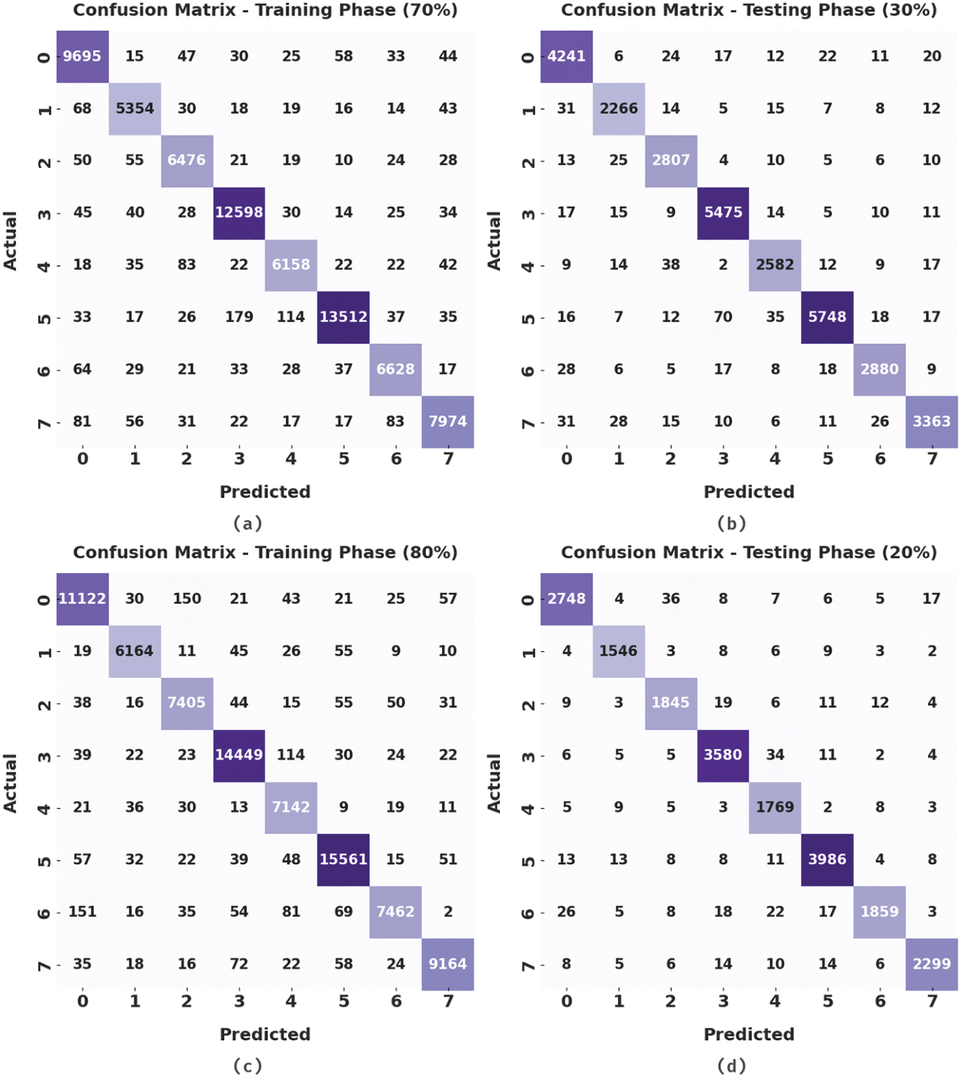
Figure 3: Confusion matrices of AOPTML-AD approach (a) 70% of TR data, (b) 30% of TS data, (c) 80% of TR data, and (d) 20% of TS data

Table 2 and Fig. 4 provide the overall classification outcomes of the AOPTML-AD model on 70% of TR data and 30% of TS data. The experimental values implied that the AOPTML-AD model had gained effectual outcomes under all classes. For instance, on 70% of TR data, the AOPTML-AD model has attained an average accuy of 99.25%, precn of 96.43%, recal of 96.87%, Fscore of 96.80%, and MCC of 96.37%.

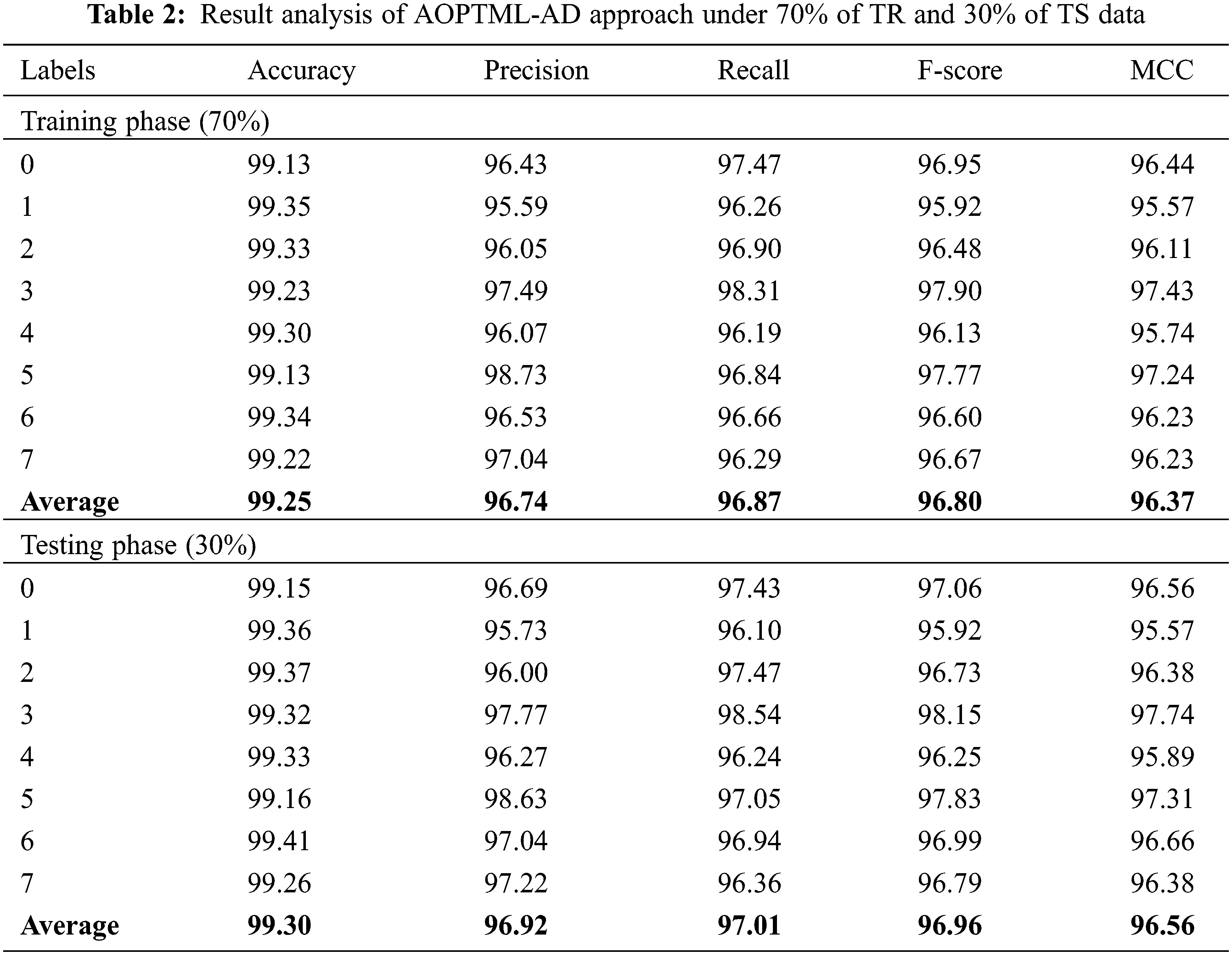
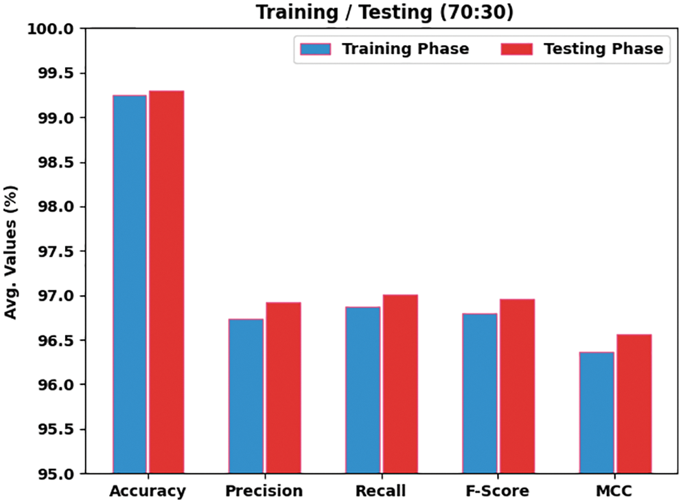
Figure 4: Average analysis of AOPTML-AD approach under 70% of TR and 30% of TS data

Next to that, on 30% of TS data, the AOPTML-AD approach has acquired an average accuy of 99.30%, precn of 96.92%, recal of 97.01%, Fscore of 96.96%, and MCC of 96.56%.

Table 3 and Fig. 5 offer the overall classification outcomes of the AOPTML-AD technique on 80% of TR data and 20% of TS data. The experimental values implied that the AOPTML-AD approach had obtained effectual outcomes under all classes. For example, on 80% of TR data, the AOPTML-AD algorithm has reached an average accuy of 99.35%, precn of 97.23%, recal of 97.22%, Fscore of 96.80%, and MCC of 96.37%. Next, on 20% of TS data, the AOPTML-AD methodology has acquired an average accuy of 99.37%, precn of 97.27%, recal of 97.30%, Fscore of 97.28%, and MCC of 96.92%.

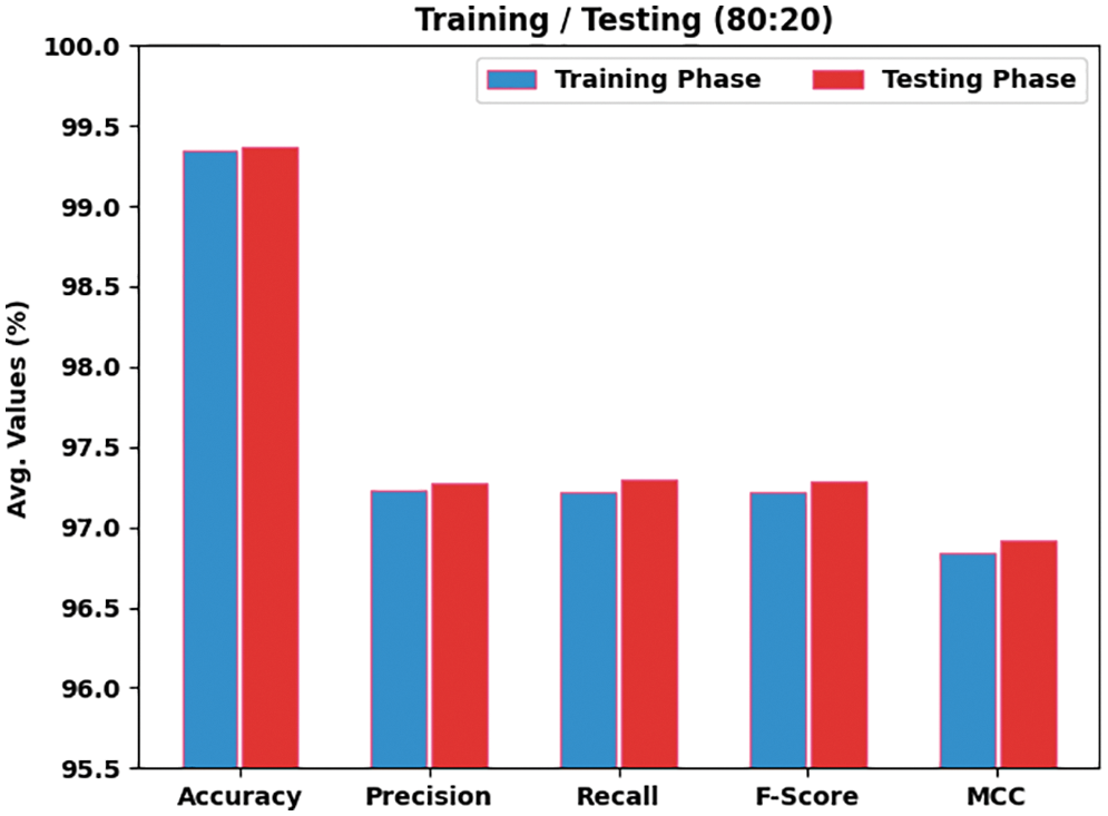
Figure 5: Average analysis of AOPTML-AD approach under 80% of TR and 20% of TS data

The training accuracy (TA) and validation accuracy (VA) acquired by the AOPTML-AD algorithm on the test dataset is demonstrated in Fig. 6. The experimental outcome denoted that the AOPTML-AD approach has achieved maximum values of TA and VA. In Particular, the VA is greater than TA.

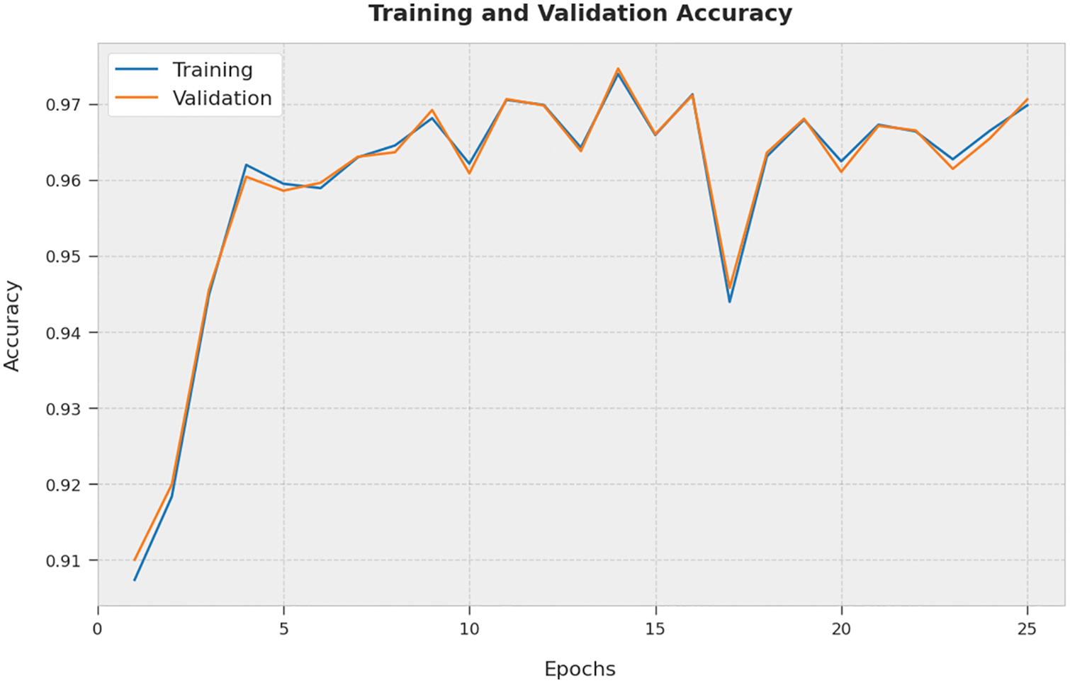
Figure 6: TA and VA analysis of the AOPTML-AD approach

The training loss (TL) and validation loss (VL) gained by the AOPTML-AD approach on the test dataset are established in Fig. 7. The experimental outcome represented that the AOPTML-AD methodology has accomplished the least values of TL and VL. Specifically, the VL is lesser than TL.

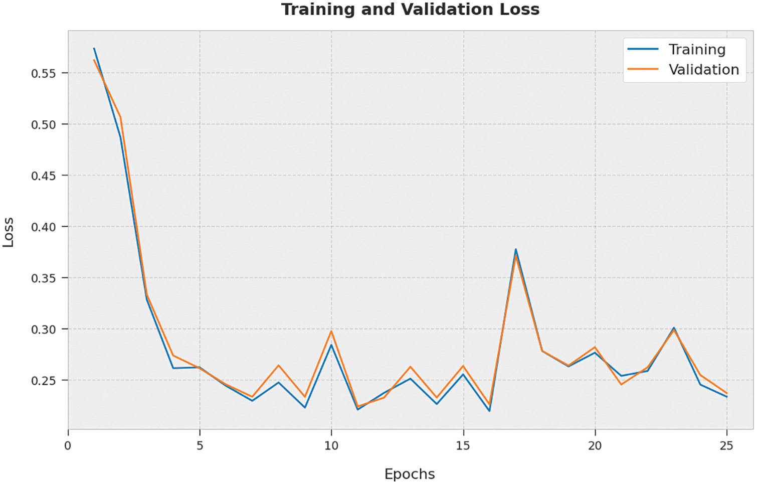
Figure 7: TL and VL analysis of the AOPTML-AD approach

A clear precision-recall analysis of the AOPTML-AD technique on the test dataset is depicted in Fig. 8. The figure denoted the AOPTML-AD approach has resulted in enhanced values of precision-recall values under all classes.

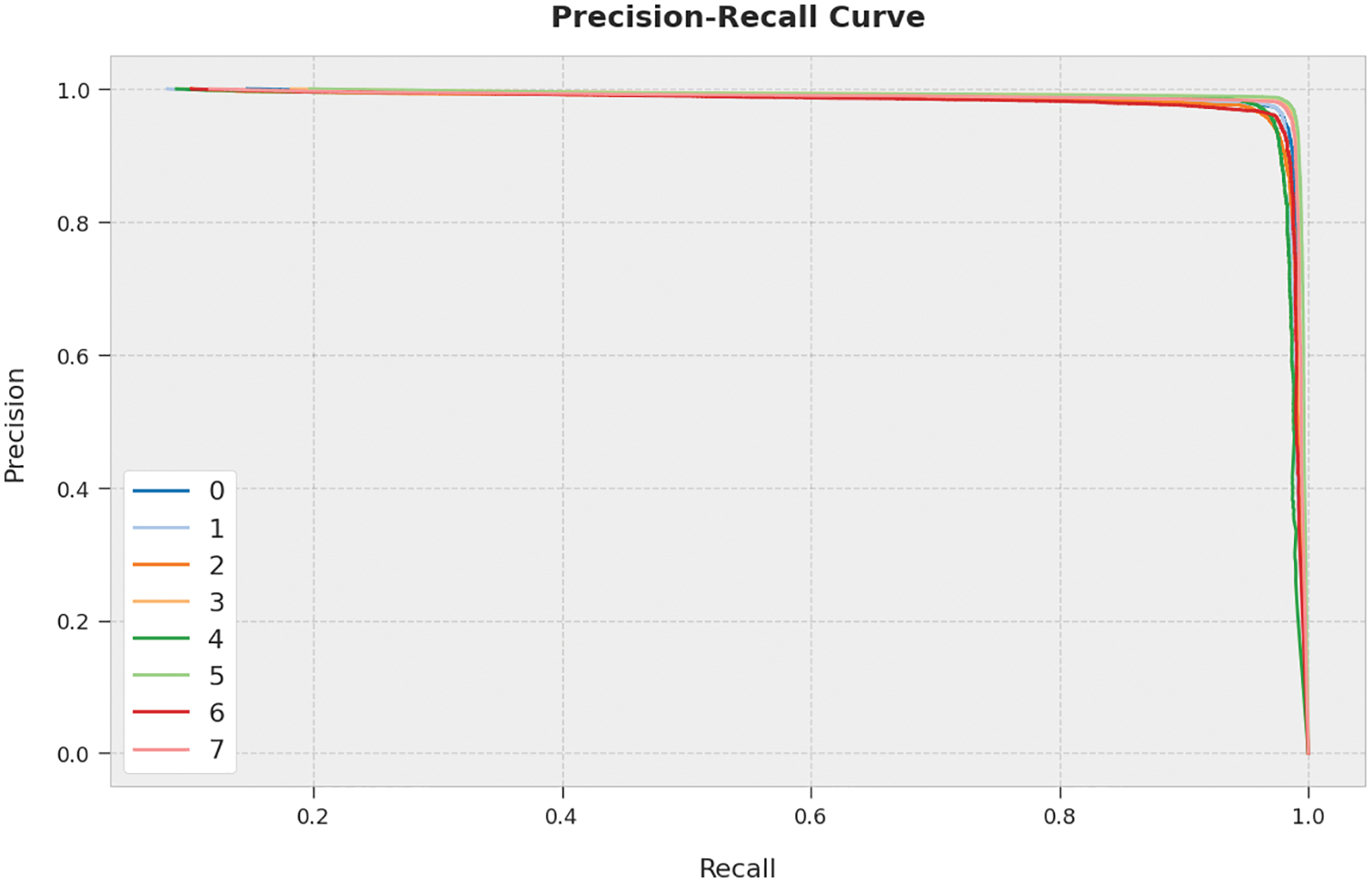
Figure 8: Precision-recall curve analysis of the AOPTML-AD approach

A brief ROC investigation of the AOPTML-AD approach to the test dataset is portrayed in Fig. 9. The results exhibited the AOPTML-AD approach has shown its ability to categorize distinct classes on the test dataset.

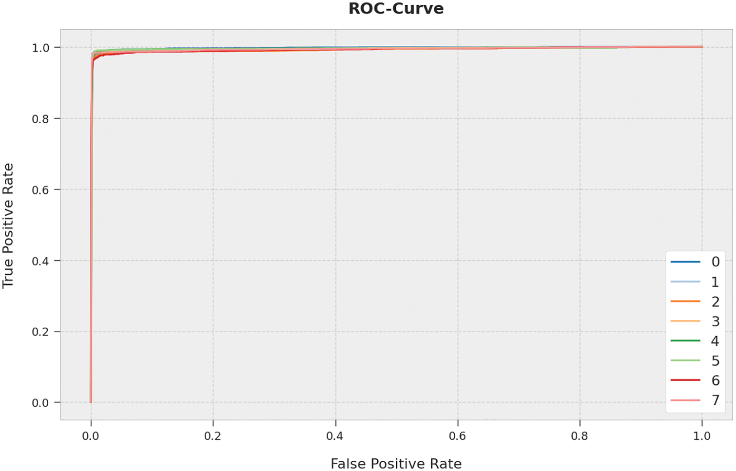
Figure 9: ROC curve analysis of the AOPTML-AD approach

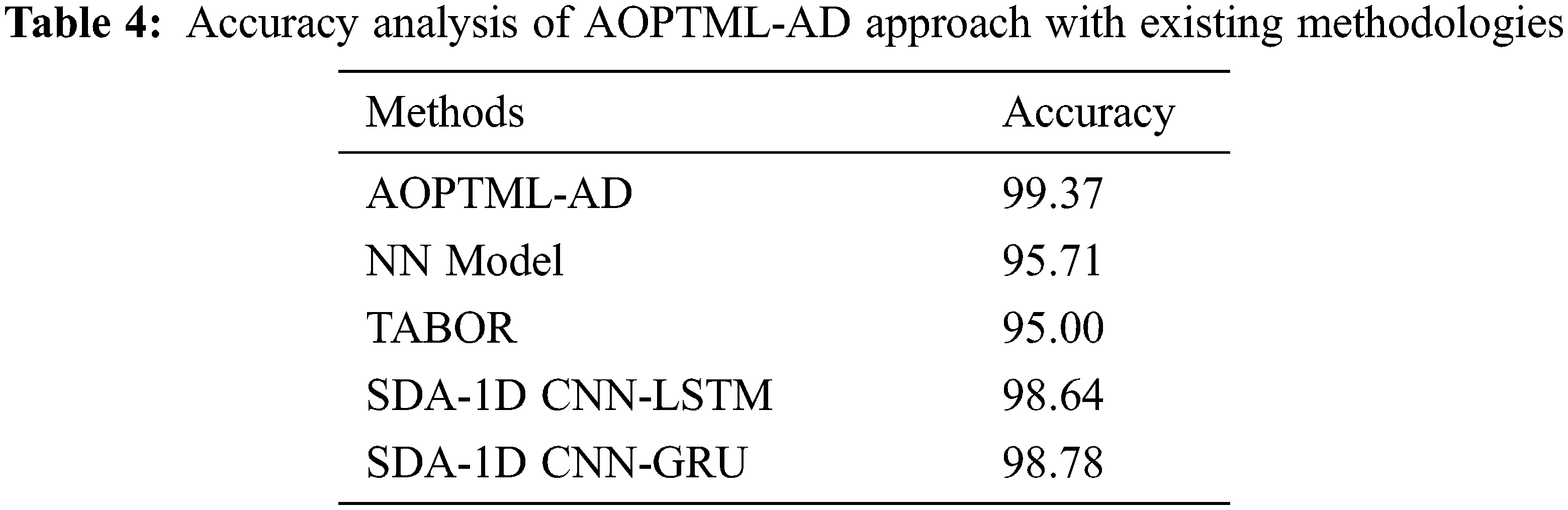
Table 4 offers a comparative accuy examination of the AOPTML-AD model with recent models [22,23]. The experimental values indicated that the neural network (NN) and TABOR techniques have resulted in reduced accuy values of 95.71% and 95%, respectively. Followed by the stacked denoising autoencoder with 1D CNN with long short-term memory (SDA-1D CNN-LSTM) model has accomplished a slightly improved accuy of 98.64%. Then, the SDA-1D CNN-gated recurrent unit (GRU) model resulted in a reasonable accuy of 98.78%. However, the AOPTML-AD model has resulted in a maximum accuy of 99.37%.

Finally, a comparative analysis of the AOPTML-AD model with the recent state-of-the-art models is portrayed in Table 5. The obtained values highlighted that the AOPTML-AD model had reported better results than other models. Fig. 10 renders a brief precn scrutiny of the AOPTML-AD method with recent models. The experimental values signified that the NN and SVM techniques had reduced precn values of 94.62% and 93.33%, respectively. Then, the STAE-AD, LSTM, and 1D CNN techniques accomplished slightly improved precn of 94.71%, 95.22%, and 95.83%, correspondingly. Then, the SDA-1D CNN-LSTM and SDA-1D CNN-GRU models have resulted in reasonable precn of 96.09% and 96.25% correspondingly. But, the AOPTML-AD model has resulted in a maximal accuy of 97.27%.

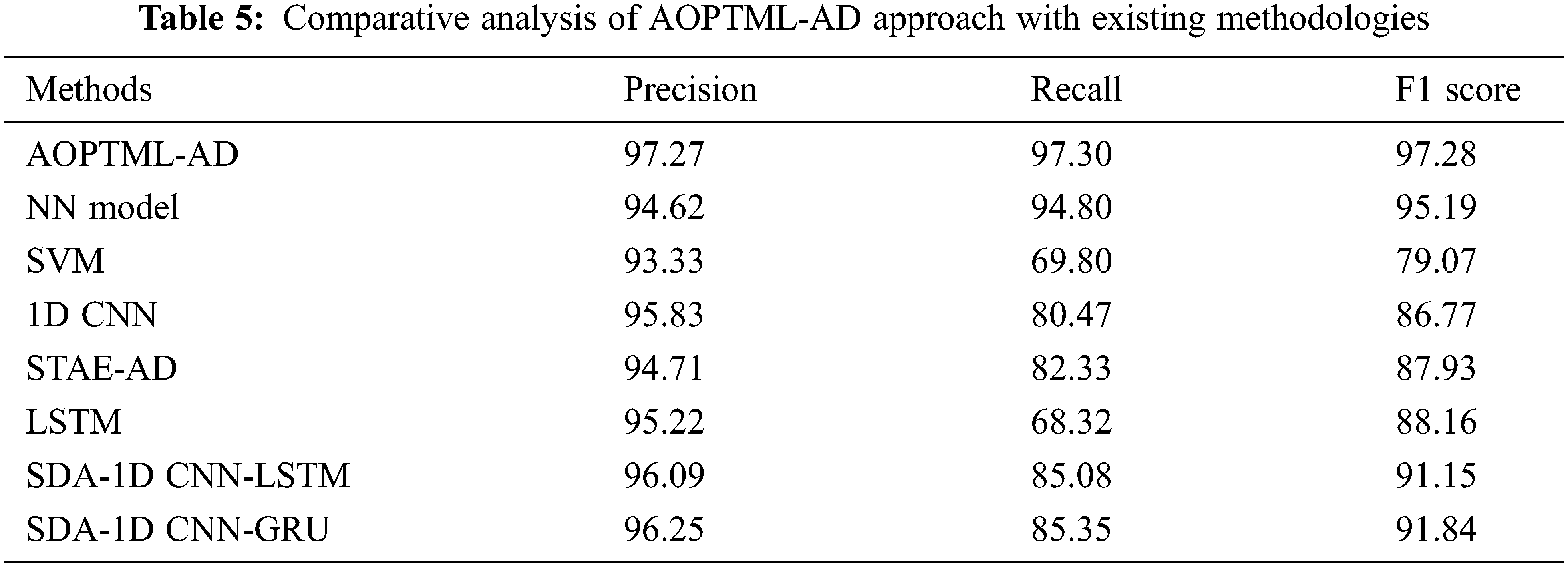
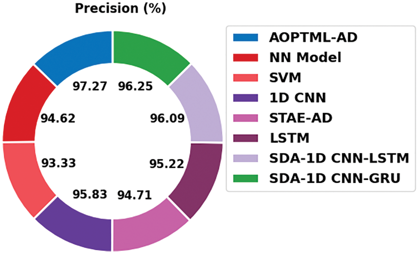
Figure 10: Precn analysis of AOPTML-AD approach with existing methodologies

Fig. 11 provides recent models’ comparative recal inspection of the AOPTML-AD algorithm. The experimental values show that the NN and SVM techniques have resulted in reduced recal values of 94.80% and 69.80%, respectively. Followed by the STAE-AD, LSTM, and 1D CNN approach has accomplished slightly improved recal of 82.33%, 68.32%, and 80.47%, correspondingly. Then, the SDA-1D CNN-LSTM and SDA-1D CNN-GRU models have resulted in a reasonable recal of 85.08% and 85.35% correspondingly. But, the AOPTML-AD algorithm has resulted in maximum recal of 97.30%.

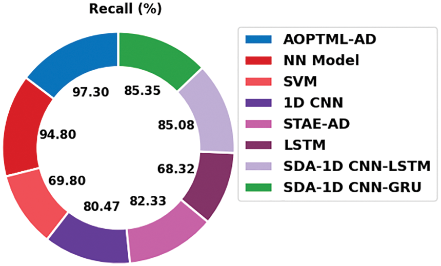
Figure 11: Recal analysis of AOPTML-AD approach with existing methodologies

Fig. 12 grants a detailed F1score scrutiny of the AOPTML-AD technique with recent models. The experimental values denoted that the NN and SVM techniques have reduced F1score values of 95.19% and 79.07%, respectively. Simultaneously, the STAE-AD, LSTM, and 1D CNN models have accomplished slightly improved F1score of 87.93%, 88.16%, and 86.77%, respectively. Afterwards, the SDA-1D CNN-LSTM and SDA-1D CNN-GRU models resulted in a reasonable F1score of 91.15% and 91.84%, respectively. But, the AOPTML-AD methodology has resulted in a maximum F1score of 97.28%.

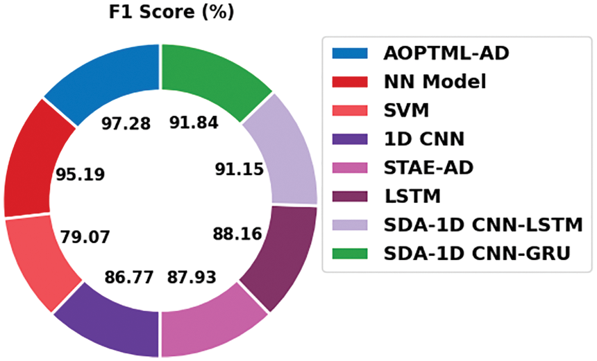
Figure 12: F1score analysis of AOPTML-AD approach with existing methodologies

The detailed results and discussion assume that the AOPTML-AD model has accomplished maximum performance over other models.

5  Conclusion

In this study, a new AOPTML-AD model intends to recognize and detect anomalous behaviour in the CPS environment. The presented AOPTML-AD framework initially pre-processed the network data by converting them into a compatible format. Followed by the IAOA-FS approach is designed to choose an optimal subset of features. Then, the ChOA with ANFIS model is utilized for the recognition of anomalies in the CPS environment. The ChOA can be applied for optimal adjustment of the MF involved in the ANFIS model. The performance validation of the AOPTML-AD methodology is executed by making use of the benchmark dataset. A detailed result analysis assured the supremacy of the AOPTML-AD approach compared to recent models with an accuracy of 99.37%. In the future, hybrid DL classification models can improve the performance of the proposed model.

Funding Statement: The authors received no specific funding for this study.

Conflicts of Interest: The authors declare that they have no conflicts of interest to report regarding the present study.

References

    1. H. M. Rouzbahani, H. Karimipour, A. Rahimnejad, A. Dehghantanha and G. Srivastava, “Anomaly detection in cyber-physical systems using machine learning,” in Handbook of Big Data Privacy, Cham: Springer, pp. 219–235, 2020. [Google Scholar]

    2. I. Priyadarshini, A. Alkhayyat, A. Gehlot and R. Kumar, “Time series analysis and anomaly detection for trustworthy smart homes,” Computers and Electrical Engineering, vol. 102, no. 20, pp. 108193, 2022. [Google Scholar]

    3. F. S. Mozaffari, H. Karimipour and R. M. Parizi, “Learning based anomaly detection in critical cyber-physical systems,” in Security of Cyber-Physical Systems, Cham: Springer, pp. 107–130, 2020. [Google Scholar]

    4. X. Jiang, W. He and T. Han, “Performance analysis and optimization of novel hybrid communication mode for vehicular network,” in 2020 IEEE Int. Conf. on Communication, Networks and Satellite (Comnetsat), Batam, Indonesia, pp. 81–86, 2020. [Google Scholar]

    5. T. S. Mohamed, S. Aydin, A. Alkhayyat and R. Q. Malik, “Kalman and Cauchy clustering for anomaly detection based authentication of IoMTs using extreme learning machine,” IET Communications, vol. 2, no. 4, pp. cmu2.12467, 2022. https://doi.org/10.1049/cmu2.12467. [Google Scholar]

    6. A. Jones, Z. Kong and C. Belta, “Anomaly detection in cyber-physical systems: A formal methods approach,” in 53rd IEEE Conf. on Decision and Control, Los Angeles, CA, USA, pp. 848–853, 2014. [Google Scholar]

    7. M. Keshk, E. Sitnikova, N. Moustafa, J. Hu and I. Khalil, “An integrated framework for privacy-preserving based anomaly detection for cyber-physical systems,” IEEE Transactions on Sustainable Computing, vol. 6, no. 1, pp. 66–79, 2021. [Google Scholar]

    8. M. Saez, F. Maturana, K. Barton and D. Tilbury, “Anomaly detection and productivity analysis for cyber-physical systems in manufacturing,” in 2017 13th IEEE Conf. on Automation Science and Engineering (CASE), Xi’an, pp. 23–29, 2017. [Google Scholar]

    9. B. Eiteneuer and O. Niggemann, “LSTM for model-based anomaly detection in cyber-physical systems,” arXiv preprint arXiv:2010.15680, 2020. [Google Scholar]

  10. P. Wang and M. Govindarasu, “Cyber-physical anomaly detection for power grid with machine learning,” in Industrial Control Systems Security and Resiliency, Cham: Springer, pp. 31–49, 2019. [Google Scholar]

  11. S. V. Thiruloga, V. K. Kukkala and S. Pasricha, “TENET: Temporal CNN with attention for anomaly detection in automotive cyber-physical systems,” in 2022 27th Asia and South Pacific Design Automation Conf. (ASP-DAC), Taipei, Taiwan, pp. 326–331, 2022. [Google Scholar]

  12. J. Goh, S. Adepu, M. Tan and Z. S. Lee, “Anomaly detection in cyber physical systems using recurrent neural networks,” in 2017 IEEE 18th Int. Symp. on High Assurance Systems Engineering (HASEI), Singapore, pp. 140–145, 2017. [Google Scholar]

  13. Y. Luo, Y. Xiao, L. Cheng, G. Peng and D. (Daphne) Yao, “Deep learning-based anomaly detection in cyber-physical systems: Progress and opportunities,” ACM Computing Surveys (CSUR), vol. 54, no. 5, pp. 1–36, 2022. [Google Scholar]

  14. S. M. Nagarajan, G. G. Deverajan, A. K. Bashir, R. P. Mahapatra and M. S. Al-Numay, “IADF-CPS: Intelligent anomaly detection framework towards cyber physical systems,” Computer Communications, vol. 188, no. 2, pp. 81–89, 2022. [Google Scholar]

  15. L. Xi, R. Wang and Z. J. Haas, “Data-correlation-aware unsupervised deep-learning model for anomaly detection in cyber-physical systems,” IEEE Internet of Things Journal, vol. 9, no. 22, pp. 1, 2022. https://doi.org/10.1109/JIOT.2022.3150048. [Google Scholar]

  16. C. Feng and P. Tian, “Time series anomaly detection for cyber-physical systems via neural system identification and bayesian filtering,” in Proc. of the 27th ACM SIGKDD Conf. on Knowledge Discovery & Data Mining, Virtual Event, Singapore, pp. 2858–2867, 2021. [Google Scholar]

  17. V. K. Singh and M. Govindarasu, “A cyber-physical anomaly detection for wide-area protection using machine learning,” IEEE Transactions on Smart Grid, vol. 12, no. 4, pp. 3514–3526, 2021. [Google Scholar]

  18. A. A. Khan, O. A. Beg, M. Alamaniotis and S. Ahmed, “Intelligent anomaly identification in cyber-physical inverter-based systems,” Electric Power Systems Research, vol. 193, no. 4, pp. 107024, 2021. [Google Scholar]

  19. Y. J. Zhang, Y. X. Yan, J. Zhao and Z. -M. Gao, “AOAAO: The hybrid algorithm of arithmetic optimization algorithm with aquila optimizer,” IEEE Access, vol. 10, pp. 10907–10933, 2022. [Google Scholar]

  20. M. S. Jalaee, A. G. Nejad, S. A. Jalaee, N. A. Zarin and R. Derakhshani, “A novel hybrid artificial intelligence approach to the future of global coal consumption using whale optimization algorithm and adaptive neuro-fuzzy inference system,” Energies, vol. 15, no. 7, pp. 2578, 2022. [Google Scholar]

  21. Z. K. Eisham, M. M. Haque, M. S. Rahman, M. M. Nishat, F. Faisal et al., “Chimp optimization algorithm in multilevel image thresholding and image clustering,” Evolving Systems, vol. 77, no. 8, pp. 195, 2022. https://doi.org/10.1007/s12530-022-09443-3. [Google Scholar]

  22. R. Taormina, S. Galelli, N. O. Tippenhauer, E. Salomons, A. Ostfeld et al., “Battle of the attack detection algorithms: Disclosing cyber attacks on water distribution networks,” Journal of Water Resources Planning and Management, vol. 144, no. 8, pp. 04018048, 2018. [Google Scholar]

  23. C. M. Paredes, D. M. Castro, V. I. Junquera and A. G. Potes, “Detection and isolation of dos and integrity cyber attacks in cyber-physical systems with a neural network-based architecture,” Electronics, vol. 10, no. 18, pp. 1–28, 2022. [Google Scholar]