Design of ANN Based Non-Linear Network Using Interconnection of Parallel Processor

1  Introduction

The ANN is inspired by the natural process of human nerve functions. The latest advances are a boom for solving high intensive calculations with more speed; human brainpower possesses high computing speed to resolve speech recognition and visualization difficulties for different domains, which no digital electronic device can effectively do to date. This ineffectiveness has driven scientists to revise the functioning of the human nervous system to propose effective neural network models that function similarly to the human brain. Currently, analog and digital included circuit technology (Integrated Circuit Technology) supplies the ability to implement hugely parallel networks of accessible processing elements. Essential emerging computing methods in very large-scale integrated circuits undoubtedly facilitate Neuron computing and avail the benefits of managing massive processing node’s conduct. ANN has gained immense popularity and has been the understudy for the past 30 years [1]. Much of the research is focused on ANN. It is gaining vast importance among the young researchers for the reason that they are a lot of improvisations in ANN, and similar algorithms were suggested by Hinton, Williams, and Rumelhart [2] also, significant improvement was suggested in the ANN theoretical concepts by Fukushima [3], Grossberg [4] and Zubair et al. [5], significantly value-added ANN methods were proposed for solving simulation problems with modified techniques [6–9]. Outstanding assessments of the past improvements in neural computation can be seen in Windrow et al. [10], and the book [11]. ANN methods offer novel methodologies to solve different tasks; ANN can be used for simulating various tasks both on traditional and advanced machines. ANN prefers using silicon VLSI to achieve extreme speed in processing inputs to get the best outputs. One of the vital things to make the best use of ANN is to propose a high-performance computing plan that can then be used to draw programs on ultra-fine parallel computers with many simple processors. The massively parallel computing system is intended to resemble brain computation characterized by significant processing and a high degree of concentration connectivity between the processing units. The technology is very scalable to support neuronal stimulation, with thousands to millions of neurons with varying degrees of connectivity or interconnection. It is anticipated that a full-scale computing system will be implemented to create a real-time simulation of over a billion neurons. To imitate brain computation, nearly one million processing cores were used concurrently. To help with the massive quantity of work that has to be done. A highly efficient asynchronous communication system is inter-neuron communication. To connect the devices, a data router network was utilized. To accomplish reliable parallel processing, the processing cores have also been grouped in individually functional and similar Chip-Multiprocessors (CMP) modelled by the structure of the brain. Each processing core has enough memory to hold the code as well as the state of the neurotransmitters as well as the chip has enough memory to store synaptic data for the system neurons connected to single neurons. The system contains enough redundancies in computation resources but instead communications network at the chip and system level to give a more excellent standard of fault-tolerant. The system enables accurate simulation of large-scale neural networks those otherwise take days to model using programs on a personal computer. This research emphasizes designing the recurrent neural network to yield optimal results in dealing with complex optimization tasks. Firstly, the theoretical foundation of ANN is analyzed and revised to get optimal solutions for solving complex tasks.

Secondly, framing of rules is carried out to design the ANN with limitations. Thirdly, the invented traditions are practiced and well demonstrated, resulting in the development of an ANN, which produces outstanding results in solving resource allocating tasks based on probabilities. The resultant ANN obtained from our proposed method simulates well in optimizing the performance of neural networks in this suggested parallel processor. This paper is divided into seven sections. In Section 1, Introduction. In Section 2, Related Work. In Section 3, Mathematical Backgrounds. In Section 4, Proposed Method of Optimization Techniques Using Neural Network and Algorithm. In Section 5, Design Example of Network. In Section 6, Experimental Approaches. And Section7, Conclusions and Directions for Future Research.

The main contributions of this paper:

•   We demonstrate that implementing complex models and significant parallel on single processor machinery is time-consuming and inefficient because a single processor must process all nodes (neurons). As a result, the computational time has increased.

•   We conclude results of various techniques or models provided throughout optimizing parallel processors in such a way that it allows for maximum output with minimal work, i.e., performance increases with a decrease in time.

•   There is a different model used for optimized neural network and efficient multi- processor.

•   ANNs can generalize and learn from examples to produce valuable solutions to these problems.

•   The data used to train ANN can be empirical data, experimental data, theoretical data, based on excellent and reliable experience, or a combination of these. The human expert can modify, verify, evaluate, or train data to introduce human intelligence. The above requirements make ANN a promising tool for modelling design activities.

2  Related Work

Since the introduction of machine learning, ANN has been on a meteoric rise, with a slew of techniques applied [12]. Emerging neural architectures training procedures and huge data collectors continually push the state-of-the-art in many applications. Deeper and more complex models are now partially attributable to rapid developments in these techniques and hardware technology. However, the study of ANN basics does not follow the same networks [13], one of the most common ANN architectures for the Computer model; most of the processors perform the same functions, except the processor, after the necessary programs and data are loaded into the processor, each processor collects a part of the neuron output in a piece of each shoulder constraint set. Each shoulder constraint must send it to the sub-processors on other processors. The sum of all other processors similarly, all other processors must collect subtotals that have been accumulated by all other processors. A lack of comprehension of its essential details [14] causes certain intriguing unexplainable phenomena to be noticed. Experiments have demonstrated that minor input changes can significantly impact performance, a phenomenon known as adversarial examples [15]. It’s also feasible to make representations that are completely unidentifiable but that convolution networks strongly believe are things. These instabilities constrain research not only on neural network operation but also on network improvement, such as enhanced neuron initialization, building, architecture search and fitting processes. Improved understanding of their qualities will contribute to Artificial Intelligence (AI) [16] as well as more reliable and accurate models. As a result, one of the most recent hot subjects is figuring out how ANN works, which has evolved into fundamental multidisciplinary research bringing together computer programmers, researchers, biologists, mathematicians, and physicists. Some of the strange ANN behaviours are consistent with complicated systems, which have been typically nonlinear, challenging to predict, and sensitive to small perturbations. Complex Networks (CN), often known as Network Science, is a scientific subject that combines graph theory, mathematics, and analytics to investigate complex systems. Its primary purpose is to examine massive networks produced from natural, complicated processes and how they relate to different neural networks, such as biological networks. Its presence of the small-world CN phenomenon, for example, has been demonstrated in the neural network of the Caenorhabditis elegans worm [17]. Following that, many learning’s discovered similar topological characteristics in human brain networks, such as magneto encephalography recordings [18], cortical connections analyses [19], and the medial reticular development of the brain stem [20]. And rules in designing the network are based on the interconnections among the hidden nodes and their learning parameters. The methodology is proven best for nonlinear resource allocation problems with a suitable design and complex issues. Neural networks yield promising results by considering many processing elements with solid interconnections.

3  Mathematical Backgrounds

This section covers the principles of CN and ANN, emphasizing the different neural network models and approaches used in this research.

3.1 Results of the Cohen-Grossberg Stability Model

A mathematical model created by Grossberg [21] includes some network models of the neuron as well as general biology and macromolecular evolution models [22–24]. Hu et al. [25] analyzed the model and found the conditions for stable convergence of the differential equation system used to characterize various standard models of neural networks. They studied dynamic systems of interdependent formal differential equations.

dxi(t)dt=−ai(xi(t)[bi(xi(t)−∑j=1n⁡tijgj(xj(t)+Ii,i=1,2,3.......,n and  t≥o (1)

where n ≥ 2 is the neurons in the network, xi is denoted the state variable associated with time (t) ith neuron, ai, bi is a continuous function and positive, Ii is the constant input from outside to the network. The n × n connection matrix T = (tij)n × n connected network, tij ≥ 0. The activation function gj is a continuous function and j reacts with input to i. They show that if all the functions ai, bi, and gj and the matrix [ tij ], these are 3 conditions are met, a system with the following equation has a Lyapunov function:

1) The symmetric matrix [ tij ] (i.e., tij = tji ) must be used.

2) With ai, the functions ai and bi must be continuous.

3) The gj functions must be increasing.

A Lyapunov function constrains the collective action of the equations that make up a dynamical system. The reason is that a mechanism to improve value evaluates the Lyapunov procedure has never been developed. When the above conditions are met, the Lyapunov process of the form Eq. (1) of interdependent differential ensures that the system follows the path of the steady-state of the initial state. As a result, the Grossberg Neural Network test is not harmful. Neural Network Work establishes the consistency of any model, which can be described by Eq. (1). Hopfield independently invented one of the event models discussed below [26].

3.2 Hopfield Neural Network Model

Hopfield used neurons in two states in his first neural network model used a model to build targeted memories in the brain. Hopfield then introduced an updated version of his older neuron that uses uninterrupted nonlinear functions to explain the outcome neuron’s behavior. Hopfield’s uninterrupted model refers to Cohen-Grossberg additive neural network mathematical model [27]. The effect in the continuous Hopfield model is determined by its level x activation; it is regulated by the distinctive equation.

dxidt=−−xiηi+∑j=1n⁡mijfj(xj) +ui (2)

where −xiηi represents the passive attenuation term, and mij represents the robustness of the relationship between neurons i.e., j and ui. Vi = fi(xi) represents the activation function of neuron j and xi represents the extrinsic input i of neuron. An activation stage xi is a variable continuous corresponding to the membrane in biological network neurons. Passive attenuation item i causes the user interface to attenuate to the side or at a certain rate proportional to η . In the absence of extrinsic input and input from other neurons xi, the output of neuron i can be represented by an average activation V rate, which corresponds to its activation function fi(xi); Vi output is in the entire range of it’s continuous. An activation function is Vi = fi(xi) connects to its user interface fi(xi). As depicted, the activation function is usually a smooth sigmoid shape. The usual choice of the equation is given

f(x) = 1[1 + tanh(Gain..x)] (3)

If you look for it meets the Cohen-Grossberg stability criterion until fj(xj) increases. Regardless of the initial state, if the external input remains constant, the network model of the neuron by Eq. (2) in due course will become flat. The height of Hopfield is high enough, and he found the Lyapunov function of n neuron network, denoted by Eq. (3), which can be expressed as. Using this theorem, the Lyapunov process of a network called “computing power” or simply “energy function” by Hoyafeld can be derived from the Lyapunov function previously identified by Cohen and Grosberg (Akça et al., 2014) draw in.

E=12∑i=1n⁡∑j=1n⁡mijfi(xi)fj(xj)−∑i=1n⁡uifi(xi) (4)

The term “energy function” comes from the comparison of network behaviors. Just as the biological system can develop towards equilibrium, the neural network will further develop towards the minimum energy function. The local minimum of the energy function corresponds to the steady-state of the neural network [28] made a breakthrough when they realized that the energy function could be calculated. Since the neural network can reduce the process of energy, the neural network can be designed to minimize the operation of combined variables in Optimization. Variable energy function problem choose the appropriate force balance value mij and external input ui. The realization of the desired network behavior becomes the neural network design to find the solution to the optimization problem. Hopfield and Tank use the power function to customize the network for various optimization problems (including hawks). The problem, signal processing problem, linear programming problem, Graphic coloring [29], Object recognition [30], safe location of the queen area, recognition of explicit isomorphism, and density determination areas of the reciprocal grid [31,32].

4  Proposed Method of Optimization Techniques Using Neural Network and Algorithm

The conceptual framework for using neural network optimization functions of networks is the energy function given by the formula [33,34].

E1=E∗(Y1,Y2,...........,Yn)+α∑i=1n⁡Pk(Y1,Y2,...........,Yn) (5)

when α > 0 is a significant scaling factor, E* is an objective function minimize, feasible and its functional elements are (Y1, Y2,……….., Yn). Considering many restrictions Y1, Y2,……….., Yn is an integer decision variable to minimize it. Assume that the condition is a non-negative penalty function Ci(Y1, Y2,……….., Yn) such that Ck(Y1, Y2,……….., Yn) = 0, if the decision variables Y1, Y2,……….., Yn then only represent E* has possible feasible solutions for k = 1, …, m.

The original bounded optimization problem can be reformulated as an unbounded subset problem. The objective is to minimize the value of E1, through the additive combination of the penalty function, feasible solution, and If (α>0) is to be large enough scale for the penalty condition, then minimizing E1 can provide a smaller solution to the original problem. E1 energy function can be expressed in the form of the given equation.

E1(Y1,Y2,...........,Yn)=−12∑i=1n⁡∑j=1n⁡mijjYiYj−∑i=1n⁡uijyi (6)

In Eq. (4), if an (α > 0) is a moderately significant scale factor for the penalty term, the minimum value of E1 will lead to a smaller feasible solution. There is a neural network corresponding to the task, and its equilibrium state is the solution. Let us imagine the objective function E* can be expressed as an equation.

Ck(Y1,Y2,...........,Yn)= −12∑i=1n⁡∑j=1n⁡mijkYiYj− ∑i=1n⁡uikYi (7)

is written in the form as energy function Eq. (6) and the boundary conditions of the problem Ck (k = 1, 2…, m) can be written as a function of energy of Eq. (7) and E* is its objective function form of the equivalent unrestricted optimization problem is according to Eq. (5),

E1=−12∑i=1n⁡∑j=1n⁡[mijj+α(mij1+mij2+…….mijn1)]YiYj−∑i=1n⁡[uij+α(ui1+ui2+….+uin1)]Yi (8)

It is worth noting that Eq. (8) is written as a function of energy

dxidt=−−xiη+∑j=1n⁡[mijj+α(mij1+mij2+…….mijn1)]Yj+[uij+α(ui1+ui2+….+uin1 (9)

Therefore, if the objective function and each constraint can be expressed as an energy function, the other energy function corresponds to an equivalent unconstrained optimization problem [35]. The energy function also determines the strength of the connection and the external input needed to activate the neural network to find the required minimum. According to Eq. (8), we can calculate the strength of network connections by adding connection strengths, which are the result of separate objective functions and constraints. The sum of the input result of the objective process and its constraints is the external input of the neuron. This discovery greatly reduces the time and effort required to estimate channel power and build an appropriate network for a specific optimization problem. Since certain types of constraints are common, a neural network architecture that implements the constraints can be created and used as a basic element for designing more complex structures. We provided a solution for the differential Eq. (8), a Lyapunov function. Since Eq. (9) defines the behaviour of the network over time, it can be opened digitally to determine the balance of the system and thus the minimum value. The effects of the objective function are summed to represent the neural connection, and the input data provided first Eq. (8). Formally, neural analysis is not an algorithm because it does not use the concept of the stepwise ordering of operations. Synonymous with programs that terminate at all inputs.

The strength of the interaction between neurons and external input determines how the network develops from its baseline to the equilibrium state of war. Rather than creating sequential programs for issues of interest, it’s better to it is better to determine the binding strength and external input during the design phase, thereby forcing the network to “flow” to balance. The solution is n/2 rule out of k. The Network Design Multiple problems neurons can be interpreted in two-dimensional or three-dimensional sequence, each neuron representing a possible true and false hypothesis. When the network is balanced, if the neuron is turned on (that is, in state 1), the relevant theory holds. This is a wrong assumption. Although neurons in optimized networks are usually designed to maintain balance in a digital state, neurons will evolve as the network develops. The output can take values in a continuous range from 0 to 1. The zero-one programming problem is an optimization problem that limits decision variables to binary values.

∑i=1n⁡Yi=k (10)

or

∑i=1n⁡Yi≤k (11)

when Y is a binary decision variable and k and n are positive integers, these problems are usually limited implements the n design rule out of k to stimulate some constraints on the energy function. This can be described as Eq. (10) or Eq. (11). The rest of this section explains how to derive the k-out of -n rule and use it as an essential element of the network architecture to enforce restrictions.

4.1 Constraint is Expressed as Equal

When the neuron expresses the hypothesis Eq. (10) requires, when the network is close to a steady-state, k out of the set of n neurons are exactly 0 ≤ k ≤ n. If the network has exactly k neurons balanced in state 1, it must have

∑i=1n⁡Ti=k (12)

where the variable of the binary solution Yi in 0 and 1 is represented by the output of a neuron

F=(k−∑i=1n⁡Ti)2 (13)

is a function of energy. If k neurons out of n neurons are in a state

∑i=1n⁡Ti(1−Ti) (14)

The number of neurons in the system is very small. However, formula Eq. (13) cannot guarantee that Ti can be digital values 0 and 1 in addition, when each Ti is either 0 or 1, the minimum is 1. The function of energy that results is

F=(k−∑i=1n⁡Ti)2+ ∑i=1n⁡Ti(1−Ti)  (15)

After algebraic adjustment and elimination of constants that have nothing to do with the minimum position, Eq. (15) can be written in the form of as energy function Eq. (14) as

F=−12∑i=1n⁡∑j=1n⁡(−2)TiTj−∑i=1n⁡Ti(2k−1) but i≠j (16)

Eq. (16) determines the strength of the relationship and the input data required to implement a steady-state network of n number of neurons with exactly or equals to k neurons.

Tij=(−2 if i≠j and 0 otherwise) (17)

ui = 2k–1 for all i

Otherwise, the combination of the term in Eq. (16) and the energy function gives Eq. (17), and If two conditions are met, a network of n number of neurons. According to Eqs. (17) and (18), it can enter a stable state by opening the knee and closing n-k neurons.

1.    Each neuron has an inhibitory effect, depending on its strength n-1 neuron.

2.    Each neuron is stimulated by stimulus signals from the outside world 2k–1.

The value mentioned above represents the relative value of the ratio force and the external input required to converge to a state where exactly n neurons are out of the k rule. In modelling or numerical research, one can simply use the values given in Eq. (17) without actually considering some implementation methods Eq. (18).

Example 1. The three neurons in Fig. 1; are connected so that the value of the input signal in state 1 exactly determines k. If k = 1, then all input neurons are in a steady state of 2k–1 = 1. One of them connected exactly three neurons. Using input data, the order in which the data is updated determines which neuron enters state 1. The constraint set is a series of neurons, which correspond to the decision variables subject to the given constraints Eq. (10). If there are multiple constraints to be run at the same time, some neurons may belong to more than one set of constraints [36], which showed that k-of-n rules could be superimposed on points that satisfy multiple conditions at the same time to obtain an energy function with a global minimum.

Figure 1: The arrow sign of each horizontal line value is -2

4.2 Inequalities as a Result of Constraints

A constraint depicted by inequality, such as Eq. (10), translates to no more than k number of neurons in an array being used.

∑i=1n⁡Yi=1 or ∑i=36⁡Yi=2 (18)

All the six neurons paired in both circle and standard circle the constraint set as the network balances out in Fig. 2 a set of n neurons can be activated. The results of Eq. (17) combined with Eq. (18) can create fewer k neurons with n network neurons in each cell. Variables Y1, Y2, Y3, and Y4 of decision slack neurons. Look at a series of n neurons reflecting hypotheses in formulating a problem to see what I mean. Fig. 5 shows a network that allows up to three or four neurons in state one. To make a sum of n + k neurons, add k number of neurons to the group. A neuron k different network, on the other hand, is hidden in the sense that it does not respond to Eq. (17) in the representation of hypotheses of the network of problems according to Eq. (18) if the force of interaction of all neuron pairs is –2, and the external input 2k–1 of each neuron. The mechanism enters the state of exactly k number of neurons. When the network is balanced, the knees should be on, and no more than n neuron of the k network hypothesized in the problem representation must be in. We will impose inequality constraints that connect neurons to the neurons of the hypothesis representation. The extra neurons are called loose neurons because they resemble flexible variables often used to solve optimization problems in operational science.

Figure 2: Intersecting collections of neurons

5  Design Examples of Network

5.1 Weapon-to-Target Assignment Problem (WTAP)

When it is necessary to allocate defensive weapons to counter offensive threats, the weapon target (WTAF) issue is a resource allocation challenge. In the WTAP version considered in this document, it is assumed that W weapons can counter n targets in T periods. It is believed that any weapon has a known chance of countering a target successfully at any time. It is also thought each target has a monetary value, that is the value of a successful neutralization represents [37]. The goal is to assign weapons to target problems to maximize the cumulative value of countered targets. The fact in Weapon-to-Target Assignment Problem is NP-complete is essential. As a result, all algorithmic approaches use heuristics to find good mappings instead of listing solutions to all possible problems (which is impossible in some cases). Formally, WTAP is a restricted nonlinear optimization problem. The protocol aims to optimize the EV or predicted value of the opponent’s targets [38],

EV = ∑jwj[1−∏t∏t(1−Pijt)Yijt] (19)

Subject to the constraint

∑j⁡∑t⁡Yit≤1 for all i (20)

&

∑i⁡∑j⁡∑t⁡Yijt≤M (21)

where, i = 1, 2, 3… Weight (w) is the index of weapon, j = 1,………., n is an index of Target, t = 1, …….., T is an index of time, wj = target j values, M is the total trip values,

Yijt=(1if  fires of weapon i target j at time t and 0otherwise),

Pijt = the probability of weapon i at time t destroy target j,

Each weapon can only fire once according to the restriction specified in Eq. (20) and shown in Fig. 3. In addition, the limit Eq. (21) defines a limit M for the total number of shots, whereby the W-M weapons can be stored for later use when the weapon i shoots at target j at time t neural network for Optimization. For illustration purposes, let’s assume that all milestones have an objective function is given by

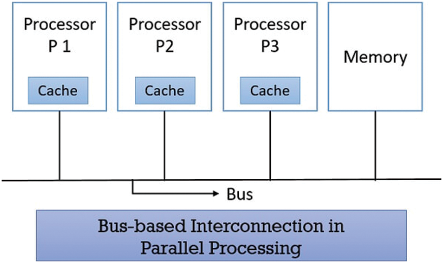
Figure 3: Hardware accelerator architecture

EV=N−∑j⁡∏i⁡∏t⁡(1−PijtYijt) (22)

For j = 1…n, wj = 1 has the same target value.

Maximizing EV is the same as minimizing ELV, the estimated amount of targets that will leak through the defense mechanism.

ELV=∑j⁡∏i⁡∏t⁡(1−PijtYijt) (23)

We can build a network that tries to reduce ELE. Whenever we equate our results with those of other researchers, we self-express our results in Eq. (22).

5.2 Objective Function Mapping onto the Energy Function

By comparing Eq. (23) with the energy function, the connection strength between a pair of neurons and the external input of each neuron can be determined. Eq. (24) The energy function can only be approximated to the objective function because it is a quadratic function and Eq. (23) has higher-order terms. Fortunately, high-level terms lose their meaning when the factors related to the objective function are converted to probabilities. The neurons in target level j represent overall combinations of armory and that time period, and the neurons consider as counter-target for target j and Eq. (23) for target j. For goal j, the contribution to the ELV in Eq. (23)

ELVj=1−∑i=1w⁡∑t=1R⁡PijtYijt+∑i=1w⁡∑t=1R⁡∑i′=1w⁡∑t′=1R⁡PijtPi′jt′YijtYi′jt′ + Higher Factor (24)

The constant 1 has nothing to do with the position of the minimum value Eq. (24) and can be excluded. In the higher-order terms ignoring in Eq. (24) and the energy function with combining the linear and quadratic terms, the approximate value of VLEj can be obtained, as shown below:

ELVJ∗=−12∑i=1w⁡∑t=1R⁡∑i′w⁡∑t′R⁡(−2)PijtPi′jt YijtYi′jt′−∑i=1w⁡∑t=1R⁡PijtYijt (25)

Although Eq. (24) is only a quadratic equation, as shown in Eq. (25), minimizing the general ELVj target has produced good results for complex battle scenarios. Otherwise, Eq. (24) is the most square. In this case, ELV and ELVj have the same minimum value. As a result, at most conservative trigger allocation strategy will lead to a better approximation of ELV. For each pair of neurons Yijt and Yi’jt’, the binding strength given by the objective function is equal to Yijt and Yi’jt’, which is the selected time. Different weapons and targets compensate j. It should be noted that the objective function only defines the connection at the j-th objective level.

VYijtjYi′jt′=−2 PijtPi′jt′ (26)

It is the required external input component, which is the result of the objective function.

UYijtj=Pijt (27)

Since j is randomly selected, Eqs. (26) and (27) apply to all j €(1,2, ……..N). The result of external input and connection has a physical explanation. Eq. (27) states that the objective function determines the external input of each neuron. The probability of Yijt dying from shooting is Pijt. It should be noted that the greater the probability that a single shot is eliminated for a given trigger hypothesis, the greater the input signal of the corresponding neuron. Therefore, when the network is balanced, the chances are greater: neurons that reflect a good record are more likely to light up, which means that a good record will be kept. Each neuron pair in the j-th layer is assigned a connection force that is twice the product of the single death probability assigned to the team, as defined in the Eq. (26), the higher the likelihood, the higher your product. Because the product will establish an inhibitory relationship between the neurons representing the shooting options for a given target, the network is unlikely to recommend the probability of shooting to high when multiple.

5.3 Constraints as a Map to the Energy Function

Only two constraints exist included within WTAP under consideration. In such a network, these restrictions can be imposed by superimposing any frameworks specified by applicable k-out-of-n rules. Weapon Shooting Restriction: A k-out-of-n rule with k = 1 could be applied for every weapon field that imposes any constraint represented as Eq. (20), thus limiting a specified weapon to firing never multiple times in as shown in its ith weapon plane or its linked slack neuron Si (Stack neuron) create a weapon constraint collection. For each weapon constraint set, employing a k-out-of-n rule using k = 1 will promote precisely one neuron to come on. Therefore, when the network equilibrates, the presence of Si implies this weapon must not be fired. The shot hypothesis neuron Yijt at weapon level i, on the other hand. The k-out-of-n rule states that every neurotransmitter, as in the problem instance, should obtain 2k–1 external perspective but must have mutually inhibiting interconnection of size 2 among constraint set’s neurons. As a result, the component due to the weapon level constraints to shot, there is still a lack of external input neurons hypotheses Yijt is, a character in the game Yijt is

UYijtwp=(2k−1)=1. (28)

Similarly, due to the weapon planes constraint, this component of external input for slack neurons Si is

UYSiwp=(2k−1)=1. (29)

The characteristic of the connection between neurons Yijt and Yij′t′ as a result of applying a k-out-of-n criterion to each weapon constraint set is

UYijtYij′t′wp=−2. (30)

The slack neuron is a type of neuron that isn’t active. Its shot-hypothesis neurons are related to Si(Stack neuron), set i with strength in weapon restriction Yijt is

UYijtSiwp=−2. (31)

Shot Limit Constraint: As stated in Eq. (21), this constraint limits the total number of weapons fired to no more than a certain number. An inequality exists when M is more excellent than M. In comparing our findings to those of others, researchers decided to impose the limitation on those previously published weapons that must be fired precisely. The strategy is reasonable; therefore, use it as soon as M ≤ W, and there are at least M nonzero shots. Kill chance in a single shot. To ensure that M shots are taken precisely because all of the necessary steps have been done, our k-out-of-n rule can be applied to the overall situation. However, this requires the creation of a group of neurons that represents shot hypotheses and a huge network of connections.

Furthermore, researchers could apply a k-out-of-n rule to the slack neurons to enforce the shot limit constraint indirectly because W−M of the slack neurons must be turned on, W−M weaponry would not be fired. By forcing W−M of the slack neurons to be on, one can ensure that exactly M shots are taken. When the k-out-of-n rule is applied to the slack neuron array, k = (W−M) indicates that each slack neuron can get the external input.

USisl=2(W − M)−1 (32)

As a result of the shot limitation constraint, the connections between every pair of different slack neurons Si and Si’ should be maintained.

MSiSi′sl=−2. (33)

In terms of link external and strengths inputs, Eqs. (26) and (33) describe the network architecture. Researchers can now create a system of equations that capture the neural behavior of both shot-slack neurons and hypotheses based on these results and Eq. (9).

5.4 Adding Up the Constraints and the Objective Function’s Effects

The differential equations that explain the generation of an activation function both to shots are presented in theory, along with slack neurons, as described by Eq. (9). It is unending, and in balancing various limitations, a number 1 was chosen in Eq. (9) and the objective function. Shot Hypothesis Neurons: Each shot hypothesis neuron Yijt has is interconnected to every neuron, including its target plan in strengths MYijtYij′t′j Eq. (26), to everyone shot hypothesis neurons including its weapon plane at strengths MYijtYij′t′wp Eq. (30), but the slack neuron within the weapon constraints sets the strengths MYijtsiwp Eq. (31). A shot hypothesis neuron’s external input consists of UYijtj Eq. (27) and UYijtwp Eq. (28). As a result, the rate of change in activity for neuron Yijt is:

dVijtdt= −Vijtη +∑i′⁡∑t′⁡MYijtYi′jt′jYi′jt′ +∑j′⁡∑t′⁡MYijtYij′t′wpYij′t′+MYijtsiwpsi+UYijtj +UYijtwp (34)

By substituting challenging values, researchers can arrive at a solution.

dVijtdt= −Vijtη +∑j′⁡∑t′(−2)⁡pijtpi′jt′Yi′jt′+ (−2)Yij′t′ + (−2)si+pijt+1 (35)

This decreases to

dVijtdt= −Vijtη +∑j′⁡∑t′(−2)⁡pijtpi′jt′Yi′jt′+ (−2)(∑j′⁡∑t′⁡Yij′t′si)+pijt+1 (36)

Slack Neurons: Its rate of growth of activation equations for slack neurons si could be established in the same way. Each slack neuron is coupled at strength MYijtsiwp to everyone cells in weapon planes i equation. Eq. (31) also with strength MSiSi′sl to other slack neurons si . Eq. (33). Slack neurons get an external input USisl from the weapon constraint set Eq. (29) and an external input USiwp from the shot limit constraint set Eq. (32). As a result, this same rate of change of activation for a slack neuron Si can be represented as

dVijtdt= −Vijtη +∑j′⁡∑t′⁡MYij′t′siwpYij′t′+∑i≠i′⁡MYsi′siwpsi′+ Usiwp+Usisl (37)

When the variables in Eq. (37) are substituted, the result is

dVijtdt= −Vijtη +∑j′⁡∑t′(−2)⁡Yij′t′+∑i≠i′⁡(−2)si′+1+2(W− M)−1. (38)

This decreases to

dVijtdt= −Vijtη +∑j′⁡∑t′(−2)⁡Yij′t′+∑i≠i′⁡(−2)si′+1+2(W − M) (39)

The behavior of shot hypothesis slack and neurons are described by Eqs. (36) and (39) accordingly. This set of equations could be used to model the WTAP network. Its gain for the neuron control system determines the value of η . It must be large enough to ensure that as the network reaches equilibrium, g (Vi) approaches 0 or 1 for every i.

6  Experimental Approaches

6.1 Mapping the Parallel Processor onto Neural Network

To map the network in the architecture of the local systems mapped in the network, the network must be divided into several DSPs on the P-Boards to maximize parallelism [39–41]. From Eq. (26), the equation of the system that describes the temporal evolution of the neurons of the fire hypothesis in Fig. 4; we can see that each neuron 1356 has a different temporal evolution [42]

Figure 4: Network performance model of a block diagram is proposed

All other neurons in its target level and all other neurons in their weapon restriction area are connected to it.

∑i′⁡∑t′⁡(−2)PijtPi′jt′Yi′jt′&(−2)[∑j′⁡∑i′⁡Yi′jt′+Si] (40)

Is the contribution to Eq. (27) within the jth goal Eq. (40), and the contribution of the restriction theorems of the ith arm is jth. It is worth noting that all interactions between neurons in the same set of weapon restrictions are weak. All needed to calculate the weapon level contribution is the number of neuron outputs in each stage of weapon restrictions Eq. (21). Once the effect of each set of weapon restrictions is calculated, if it is possible to die of a specific target in a given shot, the state of the network in the target plan is to be changed. The level is stored in the P- board processor (on local memory). The next step is to connect the processor to one or more target layers. As long as the targets do not exceed the available processors, each target level can be assigned to a different processor. By allocating an entire target plane, the processor calculates Eq. (28) without data from another processor in Fig. 3. Each set of weapon restrictions is distributed to all processors using this partitioning method. The processor only has access to a subset of the network neuron outputs needed for computation. As a result, inter-processor contact must assign the subtotals required to compute each weapon. Set constraints Eq. (28) are incorporated into the final product Eq. (27). Most of the processors perform the same functions, except the processor, which should contain the state of the neurons in the relaxation array. After the necessary programs and data are loaded into the processor, each processor collects a part of the neuron output in a part of each shoulder constraint set, and each shoulder constraint must send it to the sub-processors on other processors. The sum of all other processors is similar; all other processors must collect subtotals that all other processors have accumulated. Now the processors are synchronized. Each processor is allowed on the global bus, while other processors can receive on the global bus. A word that is of 64- bit version can be sent from one processor to another processor in one bus cycle. Both processors calculate the sum of neuron output in each set of weapon limits and start a new cycle after receiving a small part of the sum accumulated by the other processors.

6.2 Network Performance

A realistic scenario with 90 risks, 100 weapons, and 3 time periods was used to test the network. The total number of weapons used was kept to a minimum of 90. This corresponds to the shot hypothesis that 90 × 100 × 3 = 27,000 neurons were required. 100 loose neurons were used to reflect the possibility that associated weapons were absent from the shooting. It required more than 51 million network connections. The consistency of the neural network solution is compared in Table 1 to two alternative algorithms: a greedy method and a linear programming technique [43]. Using the same test condition, the three approaches were compared. To optimize EV, higher EV values mean better results. The greedy algorithm starts with no assigned shots and then searches through all eligible shots for the one that offers the most and a slight noticeable improvement in EV. Chakraborty [44] generated the result of linear programming with the linear Karmarkar method. The greedy algorithm and linear programming are deterministic approaches. The algorithm, the greedy algorithm, was executed on a 6 MIPS computer, while the linear programming approach was executed on a 41 MIPS capable parallel processor. The Loral system described above (with two P-plates) was used to obtain the neural network results. The neural network offered the best solution for the test scenario, as shown in Table 1, Figs. 4, and 5.

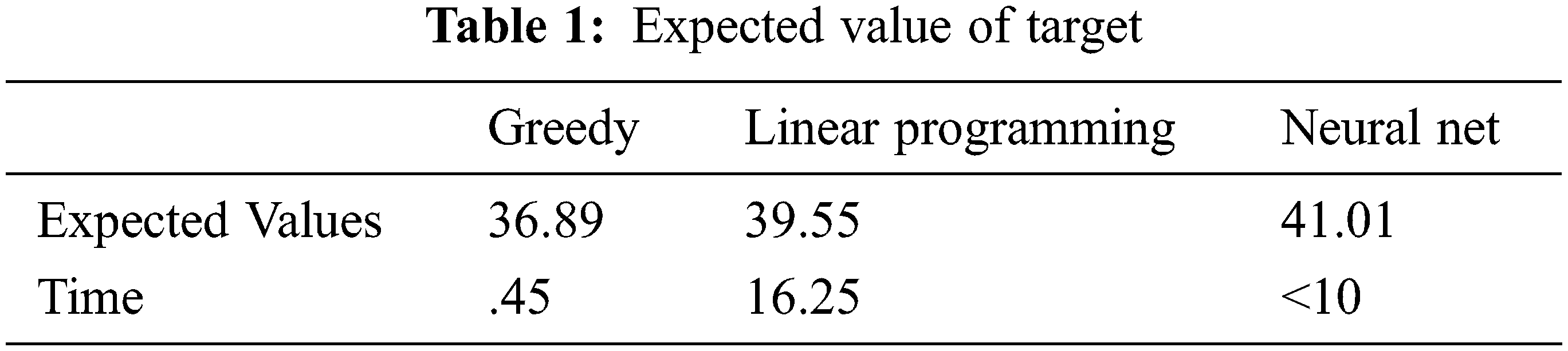
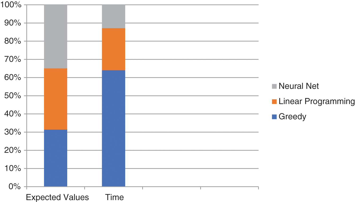
Figure 5: Neural network of cumulative performance

7  Conclusions and Directions for Future Research

In this paper, the procedure of designing ANN has been discussed precisely to attain optimized applications and presents literature work mainly based on theories to select the desired neural network for getting promising results. Most importantly, the rule k < N/2 says K (less than or equal to N) mainly focuses on the network’s behaviour based on constructing the time evolution equations. The rule k < N/2 says K (less than or equal to N) job is to Network connection strength and external inputs by Imposing constraints on equality. The rule k < N/2 says K (less than or equal to N) allows us to define the strengthened connections and external inputs and impose constraints on inequality. Take network development as an example to solve the complex problem of re-source budgeting (the trouble of optimal allocation of arms in response to threats) and explain the ANN method to optimize resources for neural network design. The artificial neural network we developed for this utility uses more than 46,000 neural factors and 49M other connections. The community has evolved from Loral Corporation to a high-performance parallel system originated specifically for applications in the neural network. The proposed ANN attained outstanding results for solving real-time application problems. The results showcase that by following theoretical procedures to design neural networks for yielding optimized solutions to solve complex problems on a large scale.

Acknowledgement: Princess Nourah bint Abdulrahman University Researchers Supporting Project number (PNURSP2022R 151), Princess Nourah bint Abdulrahman University, Riyadh, Saudi Arabia.

Funding Statement: This research is funded by Princess Nourah bint Abdulrahman University Researchers Supporting Project number (PNURSP2022R 151), Princess Nourah bint Abdulrahman University, Riyadh, Saudi Arabia.

Conflicts of Interest: The authors declare that they have no conflicts of interest to report regarding the present study.

References

1. M. A. Razi and K. Athappilly, “A comparative predictive analysis of neural networks (NNs) nonlinear regression classification and regression tree (CART) models,” Expert Systems with Applications, vol. 29, no. 1, pp. 65–74, 2005. [Google Scholar]
2. N. Srivastava, G. Hinton, A. Krizhevsky, I. Sutskever and R. Salakhutdinov, “Dropout: A simple way to prevent neural networks from overfitting,” Journal of Machine Learning Research, vol. 15, no. 1, pp. 1929–1958, 2014. [Google Scholar]
3. K. Fukushima, “Cognitron: A self-organizing multilayered neural network,” Biological Cybernetics, vol. 20, no. 3, pp. 121–136, 1975. [Google Scholar] [PubMed]
4. S. Grossberg, “Studies of mind and brain: Neural principles of learning, perception, development, cognition and motor control,” Springer Science & Business Media, vol. 70, no. 2, pp. 34–54, 2012. [Google Scholar]
5. S. Zubair and A. K. Singha, “Network in sequential form: Combine tree structure components into recurrent neural network,” IOP Conference Series: Materials Science and Engineering, vol. 1017, no. 1, pp. 012004, 2021. [Google Scholar]
6. M. Holler, S. Tam, H. Castro and R. Benson, “An electrically trainable artificial neural network (ETANN) with 10240 floating gate synapses,” International Joint Conference on Neural Networks, vol. 2, pp. 191–196, 1989. [Google Scholar]
7. M. A. Mahowald and T. Delbrück, “Cooperative stereo matching using static and dynamic image features,” Analog VLSI Implementation of Neural Systems, vol. 21, pp. 213–238, 1989. [Google Scholar]
8. M. A. A. E. Soud, R. A. A. Rassoul, H. H. Soliman, El-ghanam and L. M. E. Ghanam, “Low-voltage CMOS circuits for analog VLSI programmable neural networks,” MEJ. Mansoura Engineering Journal, vol. 28, no. 4, pp. 21–30, 2021. [Google Scholar]
9. F. Hadaeghi, “Neuromorphic electronic systems for reservoir computing,” arXiv preprint arXiv: 1908.09572, 2019. [Google Scholar]
10. B. Widrow and M. A. Lehr, “Years of adaptive neural networks: Perceptron,” Madaline and BP. Proc. IEEE, vol. 45, pp. 1550–1560, 2021. [Google Scholar]
11. A. K. Singha and P. K. Kushwaha, “Patient cohort approaches to data science using Biomedical Field,” EPH-International Journal of Science And Engineering, vol. 1, no. 1, pp. 457–462, 2018. [Google Scholar]
12. M. M. Najafabadi, F. Villanustre, T. M. Khoshgoftaar, N. Seliya, R. Wald et al., “Deep learning applications and challenges in big data analytics,” Journal of Big Data, vol. 2, no. 1, pp. 1–21, 2015. [Google Scholar]
13. S. Basu, M. Karki, S. Mukhopadhyay, S. Ganguly, R. Nemani et al., “A theoretical analysis of deep neural networks for texture classification,” International Joint Conference on Neural Networks (IJCNN), vol. 2016, pp. 992–999, 2016. [Google Scholar]
14. A. Nguyen, J. Yosinski and J. Clune, “Deep neural networks are easily fooled: High confidence predictions for unrecognizable images,” Proceedings of the IEEE Conference on Computer Vision and Pattern Recognition, vol. 27, pp. 427–436, 2015. [Google Scholar]
15. I. J. Goodfellow, J. Shlens and C. Szegedy, “Explaining and harnessing adversarial examples,” arXiv preprint arXiv: 1412.6572, 2014. [Google Scholar]
16. A. Adadi and M. Berrada, “Peeking inside the black-box: A survey on explainable artificial intelligence,” IEEE Access, vol. 6, pp. 52138–52160, 2018. [Google Scholar]
17. A. L.Barabási and R. Albert, “Emergence of scaling in random networks,” Science, vol. 286, no. 5439, pp. 509–512, 1999. [Google Scholar]
18. C. J. Stam, “Functional connectivity patterns of human magnetoencephalographic recordings: A ‘small-world’ network,” Neuroscience Letters, vol. 355, no. 1–2, pp. 25–28, 2004. [Google Scholar] [PubMed]
19. O. Sporns and J. D. Zwi, “The small world of the cerebral cortex,” Neuroinformatics, vol. 2, no. 2, pp. 145–162, 2004. [Google Scholar] [PubMed]
20. M. D. Humphries, K. Gurney and T. J. Prescott, “The brainstem reticular formation is a small-world, not scale-free, network,” Proceedings of the Royal Society B: Biological Sciences, vol. 273, no. 1585, pp. 503–511, 2006. [Google Scholar]
21. H. White and M. Stinchcombe, “Multilayer feedforward networks are universal approximators,” Neural Networks, vol. 2, no. 5, pp. 359–366, 2003. [Google Scholar]
22. H. Akça, V. Covachev and Z. Covacheva, “Global asymptotic stability of Cohen-Grossberg neural networks of neutral type,” Нелінійні коливання, vol. 14, no. 6, pp. 145–159, 2015. [Google Scholar]
23. F. Wu, “Global asymptotic stability for neutral-type Hopfield neural networks with multiple delays,” Journal of Physics: Conference Series, vol. 1883, no. 1, pp. 12089, 2021. [Google Scholar]
24. J. Hao and W. Zhu, “Architecture self-attention mechanism: Nonlinear optimization for neural atchitecture search,” Journal of Nonlinear and Variational Analysis, vol. 5, no. 1, pp. 119–140, 2021. [Google Scholar]
25. L. Hu, L. Sun and J. L. Wu, “List edge coloring of planar graphs without 6-cycles with two chords,” Discussiones Mathematicae: Graph Theory, vol. 41, no. 1, pp. 199–211, 2021. [Google Scholar]
26. J. J. Hopfield, “Neural networks and physical systems with emergent collective computational abilities,” Proceedings of the National Academy of Sciences, vol. 79, no. 8, pp. 2554–2558, 2021. [Google Scholar]
27. N. Ozcan, “Stability analysis of Cohen-Grossberg neural networks of neutral-type: Multiple delays case,” Neural Networks, vol. 113, no. 6, pp. 20–27, 2019. [Google Scholar] [PubMed]
28. E. Agliari, F. Alemanno, A. Barra, M. Centonze and A. Fachechi, “Neural networks with a redundant representation: Detecting the undetectable,” Physical Review Letters, vol. 124, no. 2, pp. 028301, 2020. [Google Scholar] [PubMed]
29. M. Alves, J. Nascimento and U. Souza, “On the complexity of coloring-graphs,” International Transactions in Operational Research, vol. 28, no. 6, pp. 3172–3189, 2021. [Google Scholar]
30. G. A. Kumar, J. H. Lee, J. Hwang, J. Park, S. H. Youn et al., “LiDAR and camera fusion approach for object distance estimation in self-driving vehicles,” Symmetry, vol. 12, no. 2, pp. 324, 2018. [Google Scholar]
31. A. K. Singha and S. Zubair, “Enhancing the efficiency of the stochastic method by using non-smooth and non-convex optimization,” Journal of University of Shanghai for Science and Technology, vol. 22, no. 10, pp. 1306–1319, 2020. [Google Scholar]
32. K. Liu, Y. Zhang, K. Lu, X. Wang, X. Wang et al., “MapEff: An effective graph isomorphism agorithm based on the discrete-time quantum walk,” Entropy, vol. 21, no. 6, pp. 569, 2019. [Google Scholar] [PubMed]
33. G. A.Tagliarini, J. F. Christ and E. W. Page, “Optimization using neural networks,” IEEE Transactions on Computers, vol. 40, no. 12, pp. 1347–1358, 1991. [Google Scholar]
34. S. Zubair and A. K. Singha, “Parameter optimization in convolutional neural networks using gradient descent,” in Microservices in Big Data Analytics Springer, Singapore, vol. 23, pp. 87–94, 2020. [Google Scholar]
35. O. I. Abiodun, A. Jantan, A. E. Omolara, K. V. Dada, N. A. Mohamed et al., “State-of-the-art in artificial neural network applications: A survey,” Heliyon, vol. 4, no. 11, pp. e00938, 2018. [Google Scholar] [PubMed]
36. M. Khishe and A. Safari, “Classification of sonar targets using an MLP neural network trained by dragonfly algorithm,” Wireless Personal Communications, vol. 108, no. 4, pp. 2241–2260, 2019. [Google Scholar]
37. J. Park, “The weapon target assignment problem under uncertainty,” Doctoral Dissertation George Mason University, 2021. [Google Scholar]
38. A. K. Singha and P. K. Kushwaha, “Speed predication of wind using Artificial neural network,” EPH-International Journal of Science And Engineering, vol. 1, no. 1, pp. 463–469, 2018. [Google Scholar]
39. R. M. Wang, C. S. Thakur and A. V. Schaik, “An FPGA-based massively parallel neuromorphic cortex simulator,” Frontiers in Neuroscience, vol. 12, pp. 213, 2018. [Google Scholar] [PubMed]
40. M. D. Jahnke, F. Cosco, R. Novickis, J. P. Rastelli and V. G. Garay, “Efficient neural network implementations on parallel embedded platforms applied to real-time torque-vectoring optimization using predictions for multi-motor electric vehicles,” Electronics, vol. 8, no. 2, pp. 250, 2019. [Google Scholar]
41. W. M. Lin, V. K. Prasanna and K. W. Przytula, “Algorithmic mapping of neural network models onto parallel SIMD machines,” IEEE Transactions on Computers, vol. 40, no. 12, pp. 1390–1401, 1999. [Google Scholar]
42. C. Peterson and B. Söderberg, “A new method for mapping optimization problems onto neural networks,” International Journal of Neural Systems, vol. 1, no. 1, pp. 3–22, 1989. [Google Scholar]
43. M. M. Khan, D. R. Lester, L. A. Plana, A. Rast, X. Jin et al., “SpiNNaker: Mapping neural networks onto a massively-parallel chip multiprocessor,” IEEE International Joint Conference on Neural Networks, vol. 67, pp. 2849–2856, 2008. [Google Scholar]
44. A. Chakraborty, V. Chandru and M. R. Rao, “A linear programming primer: From Fourier to Karmarkar,” Annals of Operations Research, vol. 287, no. 2, pp. 593–616, 2020. [Google Scholar]
Cite This Article
Copyright © 2023 The Author(s). Published by Tech Science Press.
This work is licensed under a Creative Commons Attribution 4.0 International License , which permits unrestricted use, distribution, and reproduction in any medium, provided the original work is properly cited.
Downloads
Citation Tools