Intelligent Sound-Based Early Fault Detection System for Vehicles

1  Introduction

Sound data provides scientific and engineering insights into various fields [1]. Machine learning (ML) [2] has aided tremendous developments in pattern recognition in many fields, including speech processing, image processing, and computer vision. Sound classification is a growing area of research with numerous real-world applications [3]. There are a large number of people over the world who can drive a car, but very few of them know more than that when the engine oil should be replaced. It is very critical for car users when the vehicle is broken or encounters a severe fault. They feel helpless to manage this problem if they are in some remote area or at an awkward time when no help is available. This could lead them to be overcharged [4] by car mechanics and maintenance companies. Many skilled drivers and auto mechanics can detect a problem with an engine or its components simply by listening to the sound it makes [5]. Many car companies have employed sound experts to determine potential engine faults [6]. These sound signals can be produced either from the engine part or other parts attached, i.e., tyranny, holster, brake pad, etc. These noisy sound signals can be used to detect whether the car is faulty or not. When the engine oil quality degrades and cannot provide smoothing motion to the piston, a harsh sound of the piston is produced that indicates an oil fault. The primary function of the timing chain is to operate the valves. If it is not firmly fixed, it vibrates and changes the sound. Destruction of the oil ring, first ring, or second ring may result because of crank fault. A substantial increase in peak combustion chamber pressure can change engine sound because of pressure deviation between 5°–10° in valve opening and closing [7]. When a machine runs, vibrations and sound signals are produced. These can be evaluated to get insight into the machine’s status. Each signal carries some energy and has its wavelength. These sound signals can tell us about the location and position of the source. These signals have multiple attributes. These attributes have different values. Signals are differentiated based on the importance of these attributes. Values of these signals can be different in different time intervals. As the values differ, each sound signal would have a different meaning. Figs. 1–3 shows normal and abnormal sound signals. A clear difference can be seen in the signal shape. Some speech processing techniques, such as the Hidden Markov models are unsuitable for these applications because of the lack of alphabet sounds [8].

Figure 1: Normal vehicle sound signal

Figure 2: Bad battery sound signal

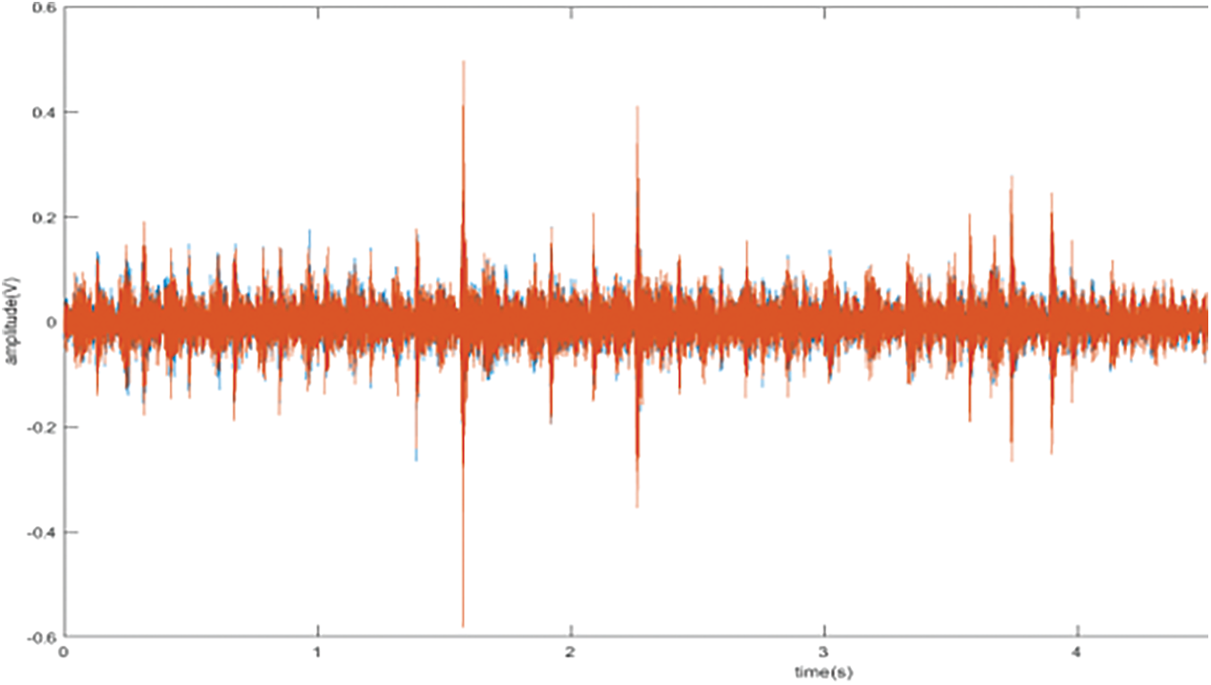
Figure 3: Engine Seize sound signal

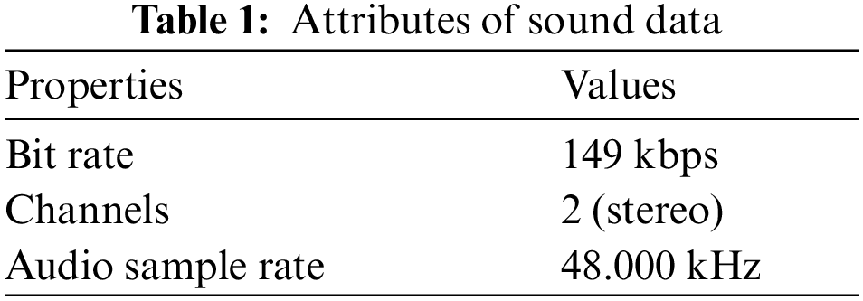
ML has been extensively used for digital signal processing to retrieve pattern information from different sound data, such as speech, music, and environmental sounds. Features play a critical role in pattern recognition. For sound signal analysis, feature extraction is essential to extracting meaningful information from the signal. Feature extraction is the process of extracting features from the signal to create a representation of the signal that is easier to process and analyze. ML is changing the medical field for the better. With its ability to quickly and accurately analyze large amounts of sound data, it is helping doctors make better diagnoses, choose more effective treatments, and even predict patient outcomes. Random forest tree, Support Vector Machine (SVM), Artificial Neural network (ANN), and Dense Neural Network (DNN) is used in the detection of different diseases from medical sounds such as heart, lungs, and breath sounds [9–14]. An automatic method [15] has been developed to classify the breathing and snoring sound segments based on their energy, the zero-crossing frequency, and the format of the sound signals. K Nearest Neighbor (KNN), fuzzy K Nearest Neighbors, along with ANN, achieved an accuracy of 99.6% on 144 samples of heart sounds [16]. Sound classification has also been used in the detection of different environmental sounds. The Gaussian mixture model [17] is a very efficient model used for the environmental sound source classification system based on Mel-frequency cepstral coefficients. A masked neural networks technique was used to classify music genres [18]. Engine sound is one of the most important aspects of a vehicle. It can indicate whether an engine is running smoothly or not. Automobile companies are now using sound analysis to study engine sounds and identify potential problems. There is little research on sound analysis using ML techniques for fault diagnosis from the vehicle. The sound signature of the car is used by [19] to detect the normal and abnormal conditions of the vehicle. An android application [20] was developed that uses Fourier transformations and spectral power density to detect problems and suggest different possible solutions. A Mel-Cepstrum, Fourier, and wavelet features-based ML technique designed that see the air filtering load of contaminants from audio data collected by a smartphone and a fixed microphone [21]. An intelligent device [22] is proposed that monitors vehicle health. This device has multiple sensors, which are connected to a microcontroller. The sensors track data, and an algorithm based on an adaptive Kalman filter is used to process the acoustic signal to determine the mode. Our study is based on these values produced from the spectrum. We searched for the vehicle sound dataset, but it doesn’t exist in standard repositories. We have used a smartphone microphone to record the voices nearby the suspected faulty engine parts. We used the “Recorder” native app that records in stereo. We used a variety of car engine sounds for the Normal and Abnormal categories. Sound files were also verified by experts for normal and abnormal categories. We analyzed those sound files and transformed them into a spectrogram that visually depicts the acoustic signals. Table 1 shows the properties of the recorded sound.

2  Methodology

We collected audio data containing vehicle sounds of different types. We applied machine learning classifiers to detect the abnormal and normal conditions of the car. If the car is in an abnormal condition, we classify the car’s sound as a specific problem. Fig. 4 shows the architectural diagram of the system.

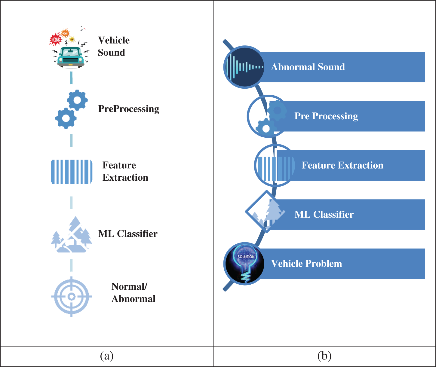
Figure 4: System architecture: (a) Normal/Abnormal sound detection; (b) problem identification

2.1 Dataset

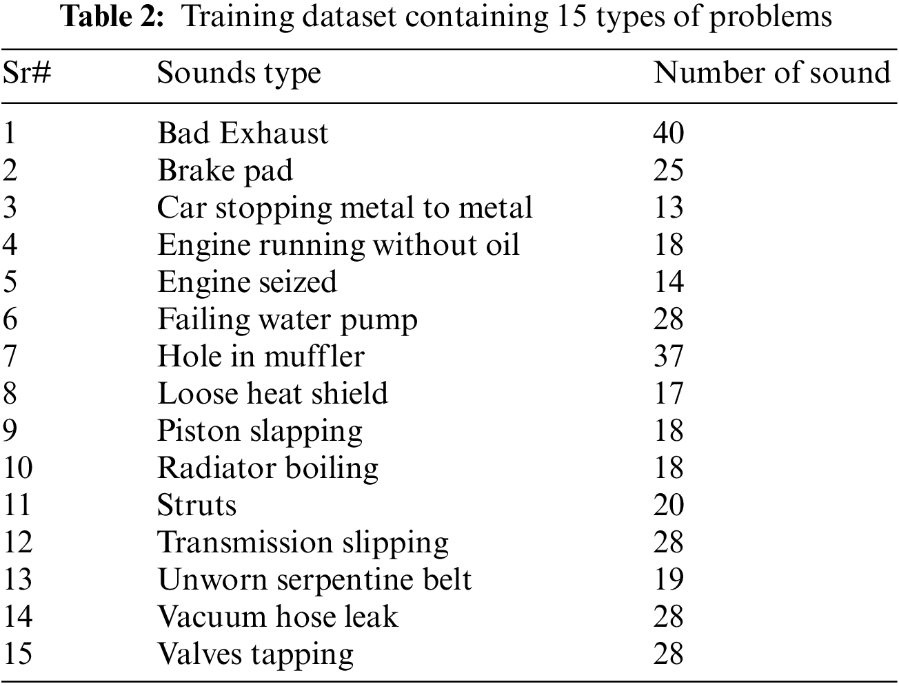
The quality of recorded audio is essential for accurate fault diagnosis. We visited many workshops, and after consulting with the resource person, we recorded the car’s audio. We tried to ensure that the audio recordings should be performed in a quiet environment to avoid environmental noise. These sound samples included a collection of an audio recording of a healthy engine and audio recordings of a faulty engine. Collecting audio samples for normal and faulty engines in various environmental conditions improves the accuracy and also aids in the diagnosis procedure being applied in real time. We collected and analyzed the sound samples of different types of cars, which represent different types of malfunctions. Although every car has different models and there are a huge number of cars available but the basic structure of cars is the same, so the noise generated by different cars is the same. We divide these audios into multiple categories according to their type. We assigned labels to these audios after consulting the experts in automobiles. We collected 351 abnormal sounds from the cars having some kind of problem, as shown in Table 2. These are engine problem sounds that can be diagnosed by expert mechanics. A knocking sound may indicate that the piston rods are loose in their cylinders, while a hissing noise may be indicative of a head gasket issue. A clicking sound could be a sign that the timing belt needs to be replaced. These sounds were used to create a learning model for the detection of abnormality in the car. We have collected 214 sounds of the normal vehicle to create a model for the detection of the normal sound of the car. We have split the files into train and testing data into different directories.

2.2 Preprocessing

We have performed the following steps of preprocessing our data to make it ready for further processing.

•   Data Formatting

•   Noise Removal

•   Data Splitting

This sound data can be noisy for a normal human being and cannot be easily categorized. Some of the data consisted of irrelevant noise, such as human voices and environmental noise. This noise in the signal affects sound data processing and may lead to faulty results. We have removed such kind of noise. A few of our data were in video format, and we extracted the audio from the video data. This extracted audio data was further converted into the .wav format. Some of the audio was in .mp3 format. This data was also converted into .wav format for further processing. Some audio sounds may have single (mono) and multiple (stereo) channels. The mono channel was also converted into stereo sounds for further processing. Data were split into normal and abnormal sounds. Equalizing the sound data is a necessary part of audio data preprocessing. This controls what it means to find spectral peaks in order of decreasing magnitude. We have performed the equalization by the following two ways.

2.2.1 Weighting Input Signal

It is done by weighting the input signal by the reciprocal of equal loudness contour listening at some nominal hearing level is a good equalization technique for audio applications. This way, the spectral magnitude ordering can be closer to perceptual audibility ordering. The audio pattern can be stabilized to provide all audio signal intervals at approximately the same amplitude (e.g., the asymptotic roll-off of all-natural spectra can be eliminated). This way, the peak finder can detect and account for all signal partials.

2.2.2 Flattening the Noise Floor

It is also a well-known equalization technique to reduce the noise from audio data. This technique is very efficient when there is a need to set a fixed track rejection threshold just beside the noise level.

2.3 Feature Extraction

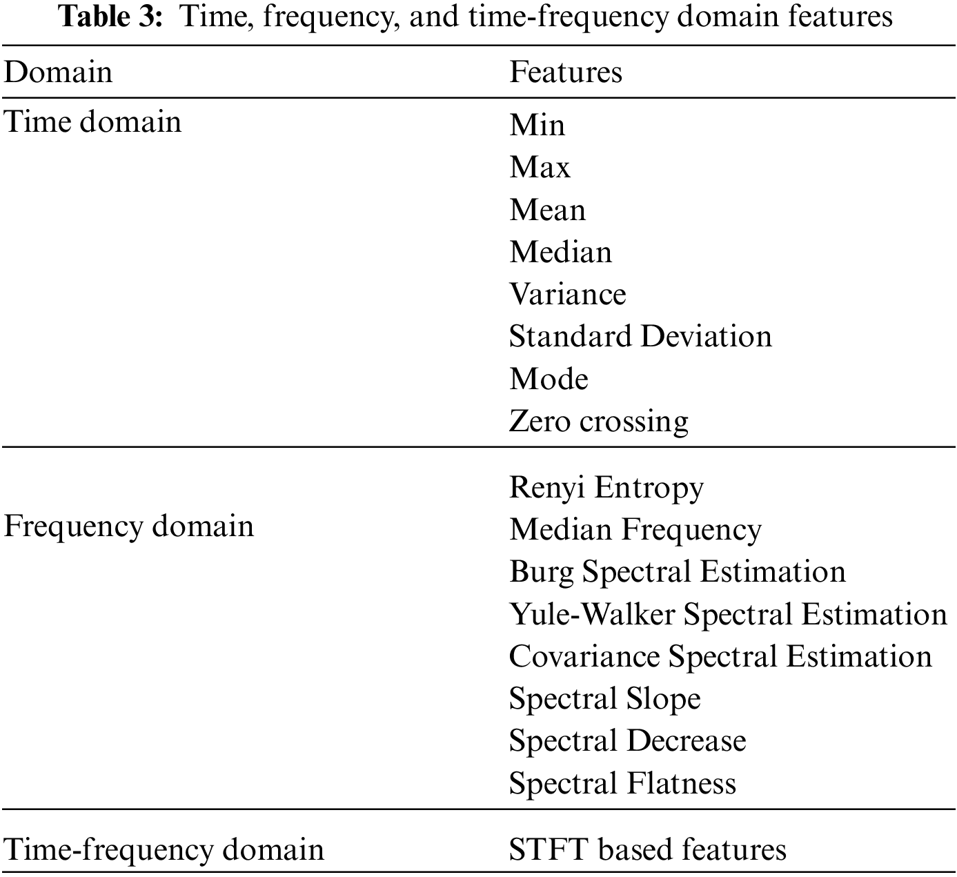
We performed three types of analysis to generate the features in our system: time domain, frequency domain, and time-frequency domain.

2.3.1 Time Domain

Analyzing the signals concerning time using different statistical functions is called Time Domain. Signals are represented in the form of real numbers. These features represent the signal’s attributes during different time intervals. We can find the magnitude of the signal over different time intervals, such as the mean value of a signal. Algorithms such as values of maximum and minimum, Wigner Ville coefficients, mean energy, zero-crossing value, spectral entropy, rényi entropy, variance value [23], arithmetic mean [23], Petrosian fractal dimension [24], median [24], standard deviation [25], skewness [25], mean curve length [25], kurtosis [25], Hjorth parameters [26], approximate entropy [26], Hurst ex-ponent [26], wavelet transform [27], and permutation entropy [28] are commonly used statistical functions for feature extraction.

2.3.2 Frequency Domain

The frequency domain is the analysis of signals using mathematical functions and operations concerning frequency instead of time. Time-domain shows only signal variations for time, but the frequency domain shows signal variations in the frequency band. It also shows the information on phase shift that must be applied to each sine wave to be capable of combining the frequency components to recover the original time signal. In this study, we calculate different features using frequency domain mathematical operations. The median of the frequency is calculated from the frequency table. We calculated these attributes in our study based on parametric modeling for the frequency domain. In the case of short signal length, parametric methods are used to produce a higher resolution. Using parametric techniques to obtain spectral estimation, these methods build a model as a linear data system by using white noise. On the base of this model, these techniques try to estimate the parameter of this linear system. All-pole model is a commonly used linear system which filters all zeroes at the origin. The methods use a process of autoregressive (AR) for the output of white noise input. For this reason, the parametric methods are sometimes called AR methods of spectral estimation.AR methods are used to represent the spectra of the data whose power spectral density is greater at specific frequencies. The Yule-Walker AR method solves the linear system and computes the AR parameters, which provide the Yule-Walker. In practice, the Yule-Walker AR method generates similar results as maximum entropy generates. A stable all-pole model is always built by the AR parameters. Another method was also used in our study for spectral estimation based on minimizing the backward and forward prediction. The Burg method for AR spectral estimation is based on minimizing the forward and backward prediction errors while satisfying the Levinson-Durbin recursion. Despite the other autoregressive estimation methods, the Burg technique avoids calculating the autocorrelation function and calculates the reflection coefficients directly. We calculate the burg on the order of 14. The covariance method for AR spectral estimation is based on minimizing the forward prediction error. The modified covariance method is based on reducing prediction errors before and after. Spectral leveling is a feature of acoustic signals that is useful in many audio signal processing applications. The spectral slope is a measure of voice quality. Perceptually, voice qualities include harsh, tense, breathy, creaky voices and whispers reflected in the intensity of the harmonics and, more generally, in the shape of the power spectrum. The spectral decrease describes the average spectral slope of the rate-map representation, emphasizing the low frequencies more strongly.

2.3.3 Time-Frequency Domain

Time-frequency domain is the true representation of the real-world signals (Short-time Fourier Transform). The completeness of the signal’s attributes can easily be observed by considering both domains. A time-frequency base analysis is often called Time-Frequency Representation (TFR). TFR fields represent the different attributes of the signal. These attributes can be amplitude or energy density. In our study, we calculate the Short-Time Fourier Transformation over the sound signal using the MATLAB spectrogram function. The set of features was recorded on the bases of the common power spectrum bands. The data was segmented into frames using a window size of 256 without overlap over which the power within each of the Delta (3–4 Hz), Theta (4–8 Hz), Alpha (8–13 Hz), Low Beta (13–16 Hz), High Beta (16–30 Hz), and Gamma (30–58 Hz) frequency bands were recorded. The filters were implemented using a short-time Fourier transform (STFT), as shown in Table 3 below.

2.4 Classification

We have three feature sets of our data for the detection of normal and abnormal sounds. We have three sets of features of car sounds consisting of fifteen different problems of cars. There are multiple ways to classify the data into certain categories we used in our study. Our system works in two steps.

•   Identification of Normal and Abnormal sound

•   Identification of problems from Abnormal sound

We have applied the random forest and the random tree for the binary classification of normal and abnormal sounds. We applied J48, random tree, and Random Forest for vehicle problem classification. Now we will present the results and comparison of signal processing techniques in these steps.

3  Experiments and Results

3.1 Detection of Normal/Abnormal Sound

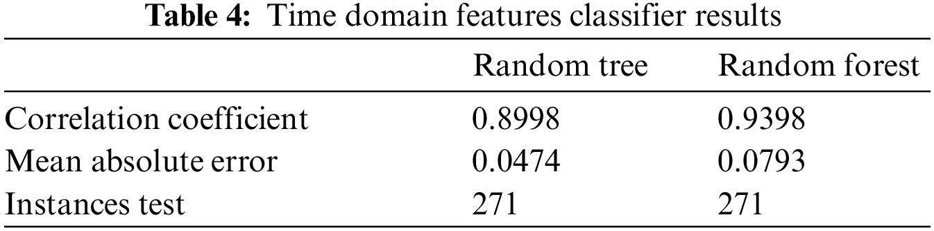
In 1st step of our study, we identified that either our vehicle was in a normal condition or an abnormal condition. We created a model based on a decision tree to classify normal and abnormal vehicle sounds. In 214 normal files, we use 108 files for training and 106 files for testing our system. If our vehicle is in normal condition, we do not need to go to the second step. Otherwise, in the 2nd step, we check which kind of problem our vehicle observes. In the learning process, 291 instances are involved. Target classes were represented as ‘1’ and ‘2’. We used ‘1’ for normal car conditions and ‘2’ for abnormal car conditions. The size of the random tree is 37. We supplied a set of 271 attributes to this model for testing. It took 2 s to test the given set of results. The summary produced after testing the supplied test on time-domain features by Random tree and Random Forest is shown in Table 4. Our model shows an 89.98% and 93.98% correlation coefficient with an absolute error of 4.74% and 7.93% on the random tree and random forest tree respectively. The correlation coefficient is used to quantify the relationship between two variables. It ranges between −1 (perfect negative correlation) and +1 (perfect positive correlation). A correlation coefficient of 0 indicates that there is no correlation between the variables. A low correlation coefficient indicates that the data points tend to clump together rather than fall along a line.

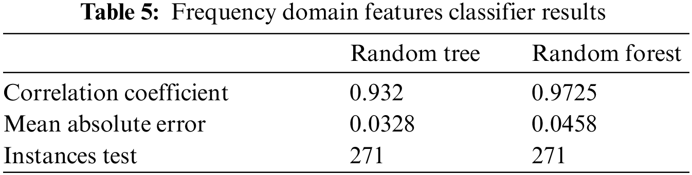
There are 104 attributes in the frequency domain feature. Weka took 0.09 s to build the model by using a random tree. After building the model, we test this model on a user-supplied test containing 271 instances. The result summary generated after testing is shown in Table 5. Our model shows a 97.25% and 93.2% correlation coefficient with a mean absolute error of 3.2% and 4.5% on the random tree and random forest tree, respectively. In machine learning, correlation indicates how well a model predicts the output variable given the input variables. A high correlation coefficient indicates that the data points tend to fall along a line rather than clump together.

Time Fourier transformation is used to record features for the time-frequency domain. We prepare a set of feature data by recording time-frequency domain features. The training set built by this technique contains 221823 instances with 258 attributes each. We test this model by supplying a test set containing 212852 instances. There are two target classes in this set which are normal and abnormal car conditions represented by ‘1’ and ‘2’, respectively. Results of the Random Forest and random tree are shown below in Table 6. Our model produces an 88% and 96% correlation coefficient with a mean absolute error of 5% on the random tree and random forest tree, which is relatively low as compared to Frequency domain features. A time domain graph lets you see what changes happen to a signal over time. A frequency domain graph shows you how much signal exists in a given frequency band.

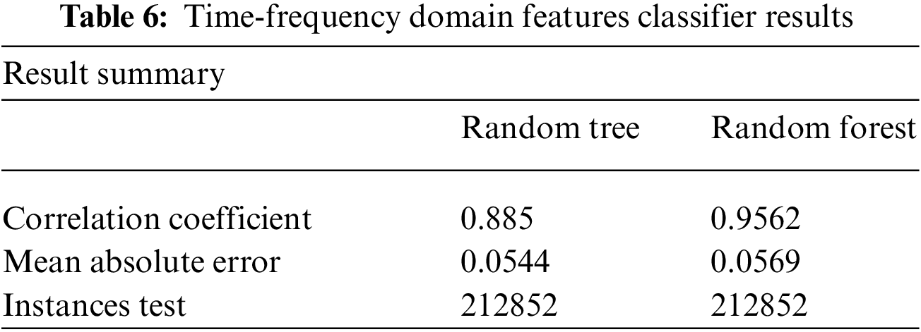
Fig. 5 shows the correlation coefficient comparison of models. The frequency-domain feature set show more than a 90% correlation of the instances of the testing set with our model. Using a frequency-domain model with a random forest classifier is highly reliable. It shows that the instances of the frequency domain features are tightly grouped and show more similarity with the model.

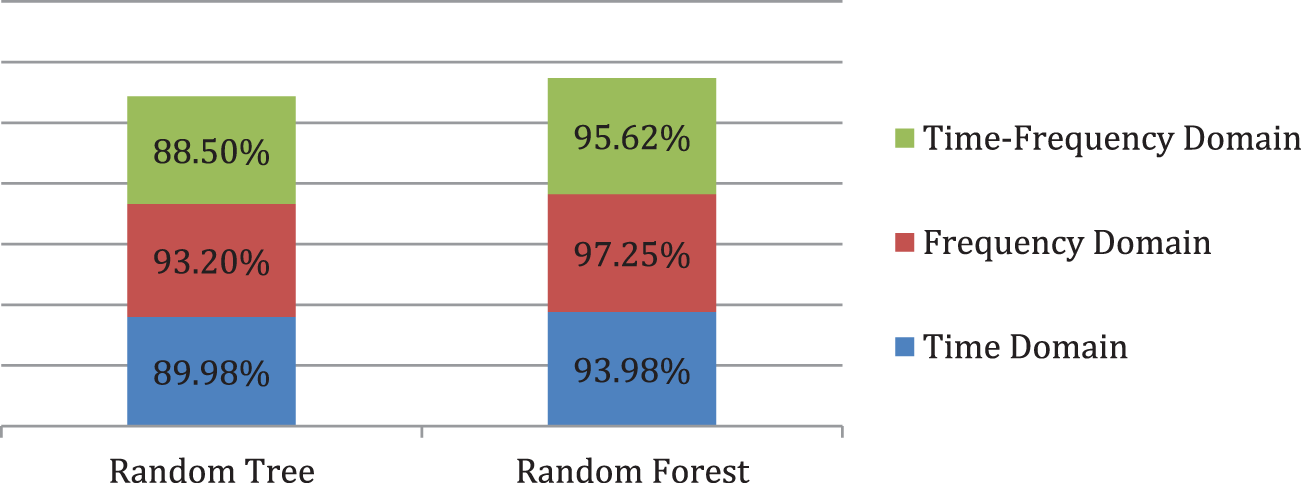
Figure 5: Correlation coefficient comparison

3.2 Vehicle Problems Classification

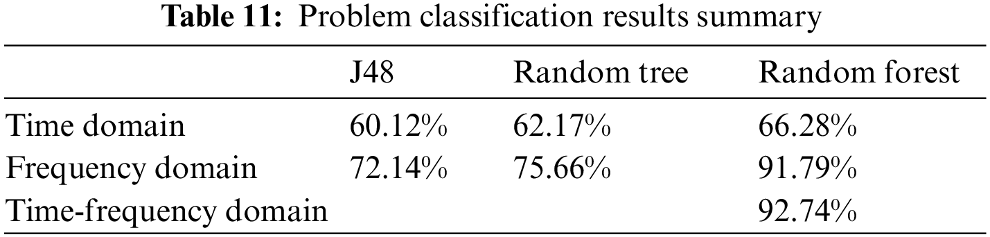
After identifying the abnormal condition of the vehicle, we further categorize the vehicle sound into 15 categories. In 341 abnormal files, we used 178 files for training purposes and 163 files for testing. We used the MATLAB tool and calculated the features using multiple feature extraction techniques, including time, frequency, and time-frequency domain. Using time-domain feature extraction techniques, we created a set of features from the audio data set of different problems. This feature set file contains all fifteen-problem data with labels. We label the data set using numbers 1–15, the same in the order of problems described in Table 1. Table 7 shows J48, random tree, and random forest classifier results using the Time domain. Out of these three classifiers, Random Forest performed better and achieved the maximum accuracy of 66%. However, this can be improved further by adding more data. Rather than making assumptions and drawing weak correlations, data speak for itself. When we have more data to work with, our models can incorporate the training data and be more accurate in prediction.

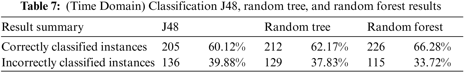
Table 8 shows J48, random tree, and random forest classifier results on the frequency domain. Results improved in the frequency domain by almost 25%. A simple decision tree combines multiple decisions. A random forest combines several decision tree classifiers and averages outputs from each to reduce predictive variance and improve accuracy. The decision tree process is fast and efficient when dealing with large amounts of data. Here our data is smaller.

Table 9 shows J48, random tree, and random forest classifier results on the time-frequency domain. Random Forest performs the best with an accuracy of 93%, and the accuracy of J48 drops to 16% only.

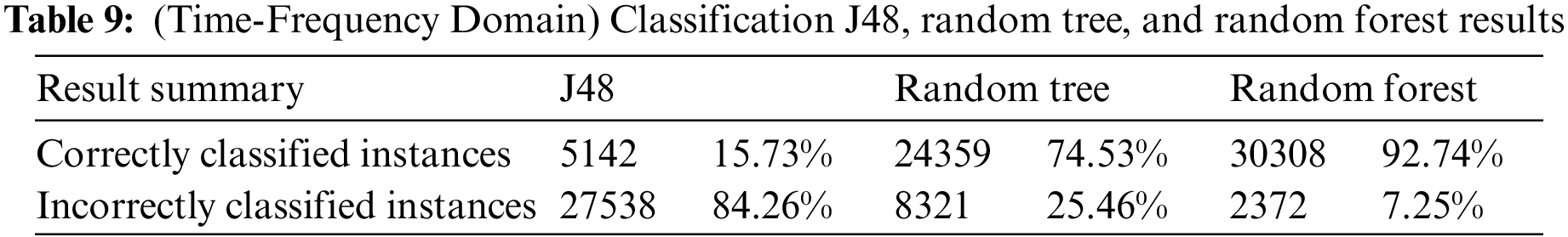
Fig. 6 shows that random forest performs the highest results on time and frequency domain features. So, we applied random forest on time-frequency domain features, and it produced the highest true positive (TP) results. It correctly classifies 92.74% of instances.

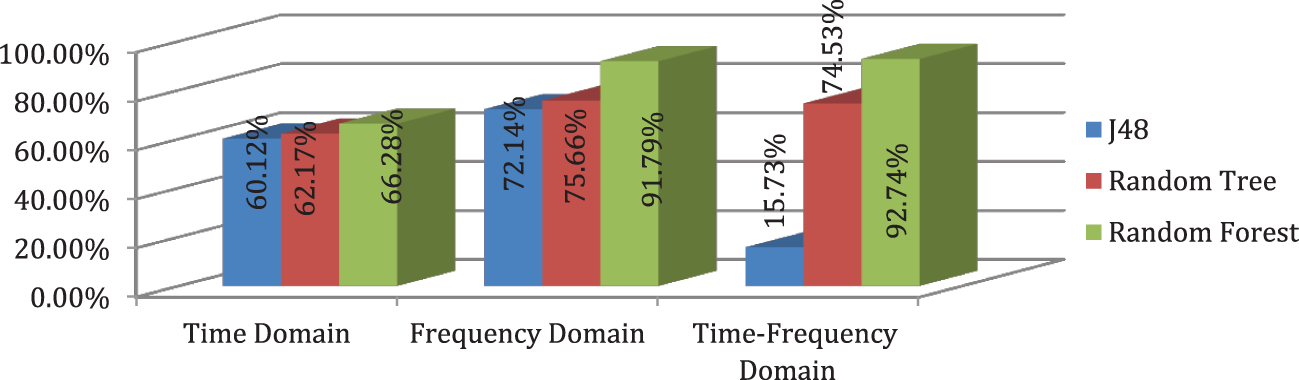
Figure 6: Comparison of different classifiers

The primary performance of the Random Forest classifier can be observed by the true positive and false positive (FP) performance measures, as shown in Fig. 7. Rate of false positive highly decreased from 33.72% to 7.25% in the Time-Frequency Domain. It is 92.74% correctly identifying the given abnormal sound file. False positive indicates the presence of the problem in normal sound. Random Forest only 7.25% classifying the normal engine sound as abnormal sound.

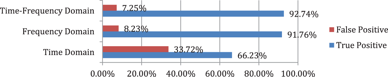
Figure 7: (Classification) Random forest TP/False positive rate

In Fig. 8 we show the performance of the random forest on all three sets of features and in the context of different performance measures. Random Forest classifier outperforms in both Frequency and Time-Frequency domains as compared to Time Domain.

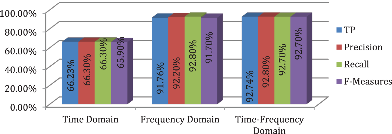
Figure 8: (Classification) Random forest different performance measures

We can conclude that Random Forest classifiers produce the best results in Time-Frequency Domain in general.

In Fig. 9, a detailed overview of the accuracy performance of the Random Forest Classifier on one of the 15 problems identified earlier is shown. As we focus on the fifteen (15) different problems. The problems are not only about the engine of the vehicle, but some noisy sounds originating from the other parts of the vehicle.

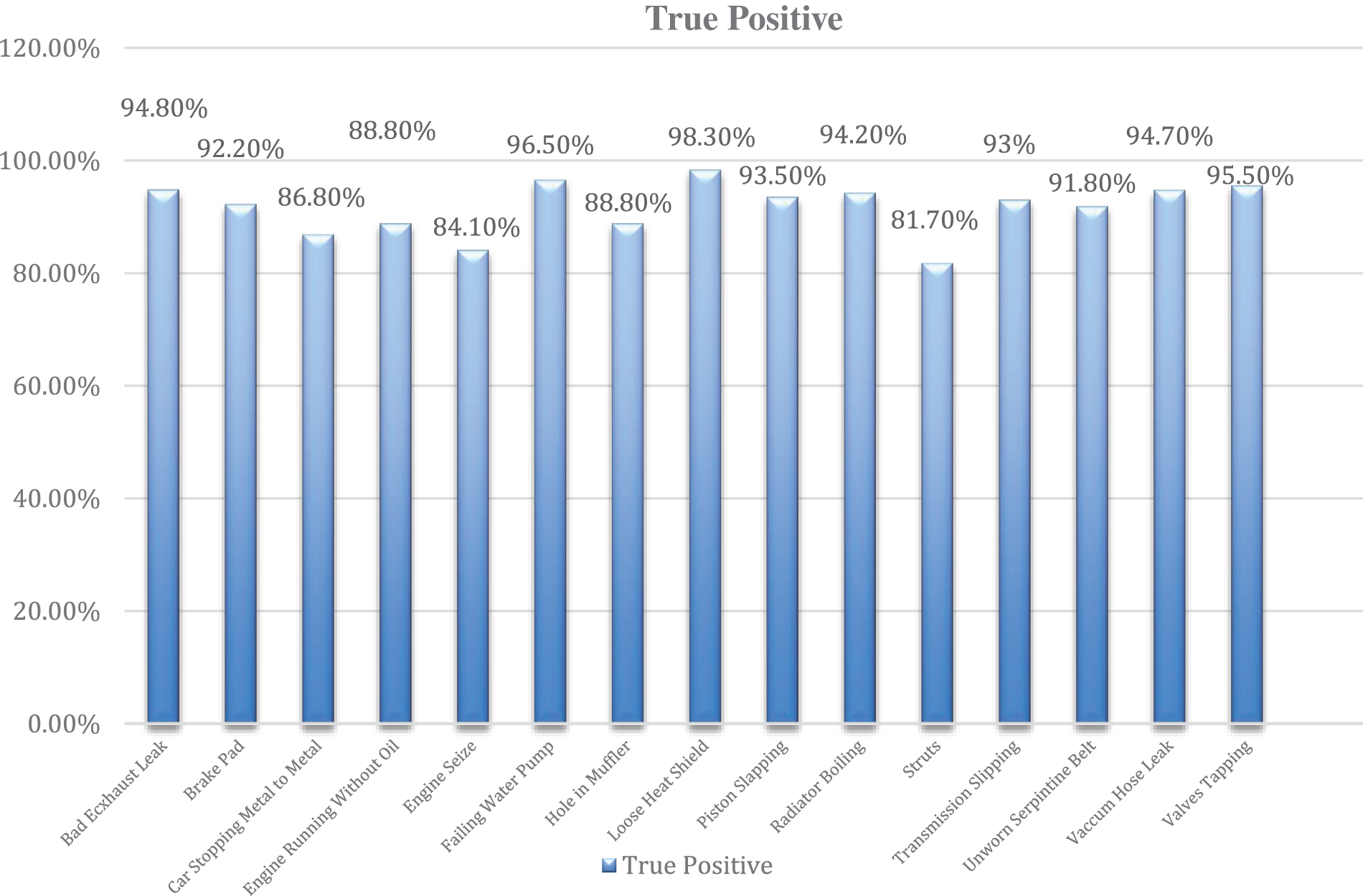
Figure 9: (Random Forest) Performance measures of different classes

It is 98.30% accurately classifying on Loose Heat Shield sound. Random Forest produces more than 90% of True positive rate on 10 different engine sound problems mentioned in Table 1. True Positive is often referred to as the sensitivity rate. The sensitivity rate for a test tells us how likely it is to be correct when given a positive result. If we have a test with a sensitivity rate of 90%, that means that if we test positive, there is a 90% chance that we have the condition in question and only a 10% chance that we do not. If a test has a false positive rate of 5%, that means that if we test negative, there’s a 5% chance that we have the condition and a 95% chance that we do not. Table 10 summarizes the accuracy of two classifiers in normal and abnormal sound detection in the time, frequency, and time-frequency domains. In this binary classification, Random Forest achieves more than 93% accuracy in all three domains. The accuracy of the Random Tree is also more than 88% for classifying the sounds into normal and Abnormal classes.

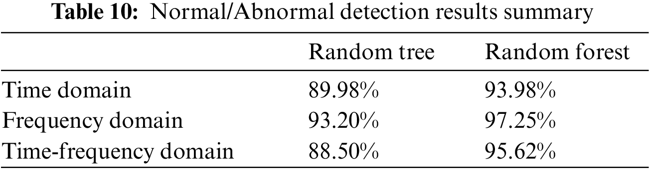
Table 11 summarizes the accuracy of problem classification on time, frequency, and time-frequency domains. These are the results of multi-class classification. There was a total of 15 problems with various numbers of data in each class. Here accuracy can be improved by adding more data to each problem set.

4  Conclusion

The increasing demand for cars with assisted driving functions and increasing penetration of electric vehicles in the market are driving the growth of the smart fault detection system market. The increasing adoption of artificial intelligence and machine learning in these systems is expected to positively impact the market’s growth. A smart fault detection system for vehicles will not only be responsible for detecting the fault but also for determining the severity of the fault, the probability of its occurrence, and the likelihood of its recurrence. It will be able to sense the operational parameters of the vehicle, compare them with the set parameters, and send a signal to the control system if there is a variation from the set parameters. The system will have artificial intelligence capabilities that will enable it to learn the pattern of normal operational parameters of the vehicle. If there is a deviation from these parameters, it will send a signal to the control system. Machine learning-based vehicle sound analysis is a new emerging applied field, and we are still looking for more research work related to this. To improve the quality of their vehicles, automobile companies like Ford are now turning to engine sound analysis. By studying the sounds produced by engines, they can identify potential issues and make necessary changes. This allows them to create better cars that are more reliable and efficient. We focused on fifteen (15) different problems. Apart from these problems, we also detected the normal and abnormal conditions of the vehicle by using our two-step method. We conducted a comprehensive study on the vehicle problem by using a more significant number of problems that are not focused on previous studies. We obtained 97.25% accuracy in detecting the normal and abnormal conditions of the vehicle. In 2nd step, we got 92.74% accuracy on fifteen various engine problems. This study can help people world wide as well as car companies, to build and deploy the smart system in the vehicle to automatically detect the problem encountered and inform the user to avoid any disturbances during their routine life. There is currently no such dataset publicly available for engine sound analysis. Without a publicly available dataset, it is difficult for research to progress in this area. Huge potential for future work is available if such a dataset is available. This type of dataset will be beneficial for researchers because it will make it easier to compare and analyze the results of different ML models. With a standardized dataset, it will also be possible to train different models and contribute to advancing this critical research area.

Funding Statement: The authors are pleased to announce that The Superior University, Lahore, sponsors this research.

Conflicts of Interest: The authors declare they have no conflicts of interest to report regarding the present study.

References

1. S. Gannot, E. Vincent, S. Markovich-Golan and A. Ozerov, “A consolidated perspective on multimicrophone speech enhancement and source separation,” IEEE Transactions on Audio, Speech, and Language Processing, vol. 25, no. 4, pp. 692–730, 2017. [Google Scholar]
2. M. I. Jordan and T. M. Mitchell, “Machine learning: Trends, perspectives, and prospects,” Science, vol. 349, no. 6245, pp. 255–260, 2015. [Google Scholar] [PubMed]
3. Z. Mnasri, S. Rovetta and F. Masulli, “Anomalous sound event detection: A survey of machine learning based methods and applications,” Multimedia Tools and Applications, vol. 81, no. 4, pp. 5537–5586, 2022. [Google Scholar]
4. P. C. Bindra and G. Pearce, “The effect of priming on fraud: Evidence from a natural field experiment,” Economic Inquiry, vol. 60, no. 4, pp. 1854–1874, 2022. [Google Scholar] [PubMed]
5. B. U. Ezeora and T. E. Ehimen, “Effect of on-board diagnostic system on fault detection in automobile on trainees’ achievement and retention in Idaw River layout area, Enugu South LGA,” Contemporary Journal of Social Science and Humanities, vol. 2, no. 5, pp. 1–9, 2021. [Google Scholar]
6. F. Thomasen, Ford Employs Specially Trained ‘Engine Listeners’ To Ensure Each New Ford Focus Rs Hot Hatch Is Running Flawlessly. Valencia, Spain: FORD MEDIA CENTER, 2016. [Online]. Available: https://media.ford.com/content/fordmedia/feu/ch/de/news/2016/03/31/ford-employs-specially-trained-engine-listeners-to-ensure-each-n.html [Google Scholar]
7. A. K. Kemalkar and V. K. Bairagi, “Engine fault diagnosis using sound analysis,” in Int. Conf. on Automatic Control and Dynamic Optimization Techniques (ICACDOT), Pune, India, pp. 943–946, 2016. [Google Scholar]
8. S. M. Bhatti, M. S. Khan, J. Wuth, F. Huenupan, M. Curilem et al., “Automatic detection of volcano-seismic events by modeling state and event duration in hidden Markov models,” Journal of Volcanology and Geothermal Research, vol. 324, pp. 134–143, 2016. [Google Scholar]
9. S. Souli and Z. Lachiri, “Audio sounds classification using scattering features and support vectors machines for medical surveillance,” Applied Acoustics, vol. 130, pp. 270–282, 2018. [Google Scholar]
10. F. Saki and N. Kehtarnavaz, “Real-time hierarchical classification of sound signals for hearing improvement devices,” Applied Acoustics, vol. 132, pp. 26–32, 2018. [Google Scholar]
11. R. Sharan and T. Moir, “Robust acoustic event classification using deep neural networks,” Information Sciences, vol. 396, pp. 24–32, 2017. [Google Scholar]
12. M. A. Islam, I. Bandyopadhyaya, P. Bhattacharyya and G. Saha, “Multichannel lung sound analysis for asthma detection,” Computer Methods and Programs in Biomedicine, vol. 159, pp. 111–123, 2018. [Google Scholar] [PubMed]
13. Z. Arshad, S. M. Bhatti, H. Tauseef and A. Jaffar, “Heart sound analysis for abnormality detection,” Intelligent Automation and Soft Computing, vol. 32, no. 2, pp. 1195–1205, 2022. [Google Scholar]
14. R. Naves, B. Barbosa and D. Ferreira, “Classification of lung sounds using higher-order statistics: A divide-and-conquer approach,” Computer Methods and Programs in Biomedicine, vol. 129, pp. 12–20, 2016. [Google Scholar] [PubMed]
15. A. Yadollahi, E. Giannouli and Z. Moussavi, “Sleep apnea monitoring and diagnosis based on pulse oximetry and tracheal sound signals,” Medical & Biological Engineering & Computing, vol. 48, no. 11, pp. 1087–1097, 2010. [Google Scholar]
16. S. Randhawa and M. Singh, “Classification of heart sound signals using multi-modal features,” Procedia Computer Science, vol. 58, pp. 165–171, 2015. [Google Scholar]
17. G. Shen, Q. Nguyen and J. Choi, “An environmental sound source classification system based on mel-frequency cepstral coefficients and gaussian mixture models,” IFAC Proceedings Volumes, vol. 45, no. 6, pp. 1802–1807, 2012. [Google Scholar]
18. F. Medhat, D. Chesmore and J. Robinson, “Automatic classification of music genre using masked conditional neural networks,” in IEEE Int. Conf. on Data Mining (ICDM), New Orleans, LA, USA, pp. 979–984, 2017. [Google Scholar]
19. M. Madain, A. Al-Mosaiden and M. Al-khassaweneh, “Fault diagnosis in vehicle engines using sound recognition techniques,” in IEEE Int. Conf. on Electro/Information Technology, Normal, IL, USA, pp. 1–4, 2010. [Google Scholar]
20. R. F. Navea and S. Edwin, “Design and implementation of an acoustic-based car engine fault diagnostic system in the android platform,” in Int. Research Conf. in Higher Education, Manila, Philippines, 2013. [Google Scholar]
21. J. E. Siegel, R. Bhattacharyya, S. Kumar and E. Sarma, “Air filter particulate loading detection using smartphone audio and optimized ensemble classification,” Engineering Applications of Artificial Intelligence, vol. 66, pp. 104–112, 2017. [Google Scholar]
22. A. Suman, K. Chiranjeev and P. Suman, “Early detection of mechanical malfunctions in vehicles using sound signal processing,” Applied Acoustics, vol. 188, pp. 108578, 2022. [Google Scholar]
23. S. Dengbo, P. Li, T. Wang, J. Hu, R. Xie et al., “DSP implementation of signal processing for two-dimensional (2-D) phased array digital multi-beam system,” in Thirteenth Int. Conf. on Signal Processing Systems (ICSPS 2021), Shanghai, China, vol. 12171, pp. 154–161, 2022. [Google Scholar]
24. N. Shoouri, “Detection of ADHD from EOG signals using approximate entropy and petrosain’s fractal dimension,” Journal of Medical Signals and Sensors, vol. 12, no. 3, pp. 254–262, 2022. [Google Scholar] [PubMed]
25. S. Pumplün and D. Thompson, “The norm of a skew polynomial,” Algebras and Representation Theory, vol. 25, pp. 869–887, 2021. [Google Scholar]
26. S. Ozsen, “Classification of sleep stages using class-dependent sequential feature selection and artificial neural network,” Neural Computing and Applications, vol. 23, no. 5, pp. 1239–1250, 2013. [Google Scholar]
27. M. Ishtiaq, M. A. Jaffar and T. S. Choi, “Optimal sub-band and strength selection for blind watermarking in wavelet domain,” The Imaging Science Journal, vol. 62, no. 3, pp. 171–177, 2014. [Google Scholar]
28. M. D’Alessandro, G. Vachtsevanos, A. Hinson, R. Esteller, J. Echauz et al., “A genetic approach to selecting the optimal feature for Epileptic seizure prediction,” in 2001 Conf. Proc. of the 23rd Annual Int. Conf. of the IEEE Engineering in Medicine and Biology Society, Istanbul, Turkey, vol. 2, pp. 1703–1706, 2001. [Google Scholar]
Cite This Article
Copyright © 2023 The Author(s). Published by Tech Science Press.
This work is licensed under a Creative Commons Attribution 4.0 International License , which permits unrestricted use, distribution, and reproduction in any medium, provided the original work is properly cited.
Downloads
Citation Tools