Modified Metaheuristics with Transfer Learning Based Insect Pest Classification for Agricultural Crops

1  Introduction

Insects are a significant factor in the world’s agricultural economy. Hence it is especially important to control and prevent agricultural insects by applying programs like insect population management and dynamic surveys with real-time monitoring systems [1]. But various species of insects in farmlands need considerable time for automatic classification by experts. It is widely known that different species of insects may contain related phenotypes, and insects frequently undertake complex phenotypes because of distinct growth periods [2]. Meanwhile, people without entomology could not differentiate the growth period of insects and insect classes; it is essential to develop effective and more rapid methodologies to overcome these problems [3].

In agriculture, pests are among the major reason for losses. Particularly, insects could be damaging since they could nourish from leaves, which affects photosynthesis, and also vectors for many severe diseases [4]. There exist numerous biological and chemical techniques for controlling pests. Also, monitoring the whole property was generally suggested to reach maximal efficiency. In several instances, monitoring can be passively done by workers as they perform their day-to-day activities. The problem with these techniques is that once the infestation can be identified, a great deal of damage might have been done previously. Earlier detection of pests needs a systematic method, particularly on huge farms. Traps are broadly accepted mechanisms for systematically monitoring pests [5]. These devices could effectively sample insect populations, if implemented appropriately, over the area of interest [6]. Therefore, it is essential to assess the status of pests accurately, autonomously, and quickly regardless of the adoption of traps or not.

Machine vision is used in plant disease recognition, insect pest detection, fruit grading, and monitoring of crops and soil. Currently, considerable progress has been achieved in the agriculture field, with the help of machine learning (ML) to classify and detect insects in stored grain conditions [7]. Vegetables and Fruits quality assessment is done using computer vision-based quality inspection encompassing classification, acquisition, segmentation, and feature extraction. The moment invariant technique was used to extract shape features, and a neural network was established to categorize twenty kinds of insect images [8]. Pest detection in a complicated background through deep residual learning has been proposed to increase the detection accuracy for ten crop insects. A multi-level classification framework and unsupervised feature learning method have been introduced for the automated classification of crop pests [9]. A current study [10] reported that image processing had been effectively used for detecting insects because of fast detection, lesser computational cost, and easier to differentiate insects.

This study introduces a Modified Metaheuristics with Transfer Learning based Insect Pest Classification for Agricultural Crops (MMTL-IPCAC) technique. The presented MMTL-IPCAC technique applies contrast limited adaptive histogram equalization (CLAHE) algorithm for image improvement. The neural architectural search network (NASNet) model is applied for feature extraction, and a modified grey wolf optimization (MGWO) algorithm is employed for the hyperparameter tuning process. At last, the extreme gradient boosting (XGBoost) model is utilized to carry out the insect classification procedure. The simulation analysis of the MMTL-IPCAC algorithm is tested on a benchmark dataset, and the outcomes are inspected in distinct prospects.

The rest of the paper is organized as follows. Section 2 offers the related works, and Section 3 introduces the proposed model. Later, Section 4 provides experimental validation, and Section 5 concludes.

2  Literature Review

Ramalingam et al. [11] formulated a remote insect trap monitoring and detection technique with DL and IoT architectures. The presented architecture is created through IoT and Fast RCNN, and ResNet50 unified object detection architecture. The Fast RCNN-ResNet 50 object detection technique is well-trained by built environment insect and farm field insect images and positioned in IoT. Kasinathan et al. [12] focused on the classifier of crop insects by using knowledge-based and machine vision methods with image processing through distinct feature descriptors involving color, texture, shape, and global image descriptor (GIST), and histogram of oriented gradients (HOG). Incorporation of the feature was utilized in the insect classification. In the study, various ML techniques involving ensemble and base classifiers were employed for three distinct insect data sets, and the performance of classifier outcomes was estimated using majority voting.

Li et al. [13] developed an automated pest detection technique based on Vision Transformer (ViT). To prevent over-fitting, the plant disease and insect pest datasets are optimized using techniques like Laplacian, Gamma Transformation, Histogram Equalization, Retinex-SSR, Retinex-MSR, and CLAHE. Later, utilize the improved dataset for training the created ViT NN for realizing the automated classifier of insect pests and plant diseases. Shi et al. [14] propose an enhanced DNN-based RFCN to resolve the classification and detection problems of eight common stored grain insects. In the study, the researcher uses the multi-scale training model using an FCN for extracting additional features of the insects and offering the position of possibly stored grain insects via RPN from the feature maps. Kuzuhara et al. [15] developed two-phase detection and identification techniques for smaller insect pests, according to CNN. Further, the researcher presented an RPN for insect pest recognition using YOLOv3 and developed a re-detection technique with the Xception module. For training those modules, the researchers presented a data augmentation technique with the help of image processing.

Huynh et al. [16] developed the CDNN technique for insect classification related to NN and DL. Firstly, insect images are gathered and extracted according to the Dense Scale-Invariant Feature Transform. Next, Bag of Features was utilized for image representation as a feature vector. Finally, the feature vector is trained and categorized using the CDNN module based on DNN. Xia et al. [17] introduced a CNN mechanism for resolving the challenge of multiclass crop insects. The technique uses NN to extract multifaceted insect features widely. In the regional proposal phase, the RPN was accepted instead of a conventional selective search approach for generating a small number of design windows that are particularly significant for accelerating computations and enlightening prediction accuracy.

3  The Proposed Model

This study has formulated a new MMTL-IPCAC approach for insect pest classification to improve agricultural pest control and crop productivity. Initially, the MMTL-IPCAC technique employed the CLAHE technique for image enhancement. The NASNet model is applied for feature extraction, and the MGWO algorithm is employed for the hyperparameter tuning process. At last, the XGBoost model is utilized to carry out the insect classification procedure. Fig. 1 illustrates the block diagram of the MMTL-IPCAC system.

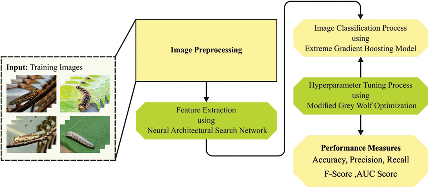
Figure 1: Block diagram of MMTL-IPCAC system

3.1 Contrast Enhancement Process

AHE (Adaptive Histogram Equalization) denotes a digital image processing method that improves the contrast of input imageries. It differs from normal HE by calculating many histograms that correlate to a certain region and using them to recreate brightness values. CLAHE is an innovative version of AHE. This prevents the over-amplification of noise that leads to the AHE model. CLAHE uses a contrast amplification limiting process that can be employed for every adjacent pixel later to form a transformation function for reducing the noise problem [18].

3.2 Feature Extraction Process

In this stage, the NASNet method is employed for feature extraction purposes. One of the most prominent DL techniques is CNN, which uses a convolutional layer rather than matrix multiplication. It is more commonly applied to categorize objects based on image datasets [19]. A CNN is made up of three layers. The input layer generates an artificial input neuron that prepares the initial dataset for the following processing. The hidden layer serves as a connection between the output and input layers, with the output layer generating results for the input layers. A CNN layer serves as this model’s key component [20]. Once a filter is employed for the input, the outcome is activation, which is the underlying convolution process. A feature map is constructed after many iterations of the same filter to the same input that shows the location and intensity of the detected patterns in the input, along with an image of the pattern. Yet, the pooling layer is another component of the CNN method. The pooling layer assists in minimizing the proportion of the feature set. Consequently, the amount of network processing and the number of learning parameters are decreased. The pooling layer adds features to the feature map via a convolutional layer in a certain region [20].

The CNN comprises eighteen layers: 3 max-pooling layers with 2 × 2 pool size, three 2D convolution layers (2DConv), two dropout layers with a 0.5 dropout rate, two dense layers, four activation layers with ReLU function, and three batch normalization layers. The CNN models’ initial layer comprises a 2DConv layer with 3 × 3 kernels and 256 filters. The activation layer, including the ReLU activation function, accompanies this 2DConv layer. Subsequently, a max-pooling layer having a pool size of 2 × 2. After the max-pooling layer, the batch normalization layer is deployed with axis 1. There is again a 2DConv layer with sixty-four filters, and the final 2DConv layer comprises 16 filters. Then, the Adam optimizer and binary cross entropy loss function was applied to compile the CNN method. Eventually, the module fitted with twenty-five epochs.

NASNet is a neural structure, and CNN is trained on around billion images from ImageNet and categorized into 1000 object types, namely pencil, keyboard, and mouse. Consequently, the network learned a rich feature representation for different images and image input of the 331 × 331 sizes. The next model performs a feature extraction extractor by eliminating the FC layers of the original pre-trained network. Like CNN, NASNet was uncompressed with the BatchNormalization layer as stem-bn1, Conv2D layer as stem-conv1, fully connected layers, and AveragePooling2D as a normal-right40 layer. Still, NASNet depends on cells or blocks that the researchers do not predetermine by the RL technique. Therefore, it comprises reduction and normal cells.

Then, we exploited the NASNet model as a feature extractor that considers 3 variables; the initial one is the weight variable which sets Imagenet as the value. The next variable parameter was include-top, whereby we involve the FC layer at the topmost network and set it at False since the feature should be extracted. At last, the variable was the input shape of the input image; for loading Imagenet weight, the input shape should be 331 × 331 × 3, which implies the 3 inputs channels, correct width, and height. So, resize each image to 331 × 331 sizes in image preprocessing. Afterwards deriving the feature, the image dimension becomes 11 × 11 × 4032, and this is because of the reduction cell since the initial layer of NASNet comprises a stride of 2 and kernel of 3 × 3. This was a feedforward method whereby the activation from the pooling layer, the final convolution layer, can be utilized on the whole images for obtaining feature representation of the cobalt or copper raw mineral images. Therefore, a convolutional feature vector can be obtained using dimensionality.

3.3 Hyperparameter Tuning Process

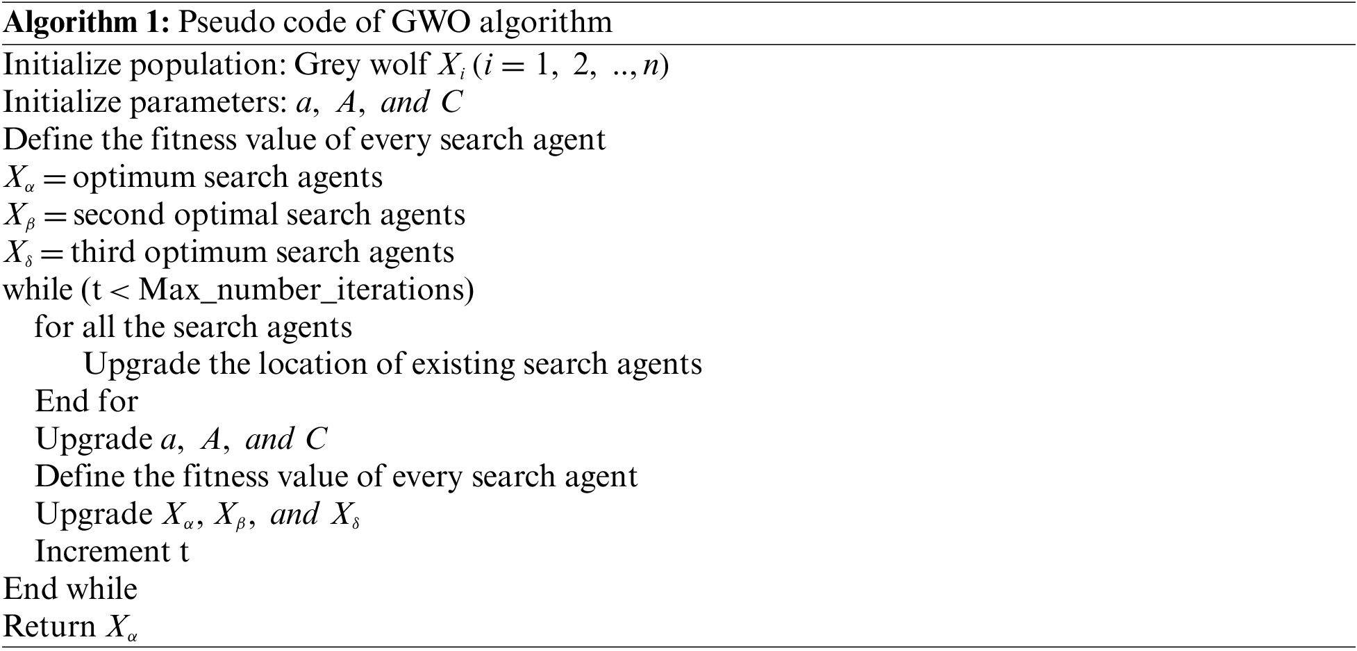
For optimal hyperparameter adjustment process, the MGWO model is exploited. Mirjalili et al. [21] established a new SI-optimized technique called GWO. Indeed, it is an original method that accelerates GW’s hunting and social hierarchy by default. For proposing the social performance of GW, it is classified into 4 states, namely α, β, δ, and ω. α considering the optimal solution implemented by β and δ, and the remaining solution derived in ω. The primary 3 fittest wolves, termed α,β, and δ, are neighbouring the prey supports ω to identify the food from the critical area. In the surrounding step, the wolf rises the location of β, or δ, as demonstrated below:

D→=|C→⋅X→p(t)−X→(t)|(1)

X→(t+1)=X→p(t)−A→⋅D→(2)

From the expression, t indicates the existing iteration, X→p(t) epitomizes the current location of prey, and X→(t) shows the present location of wolves. D→ denotes the distance between wolf and prey, and co-efficient vectors A→ and C→ result from mathematical models.

A→=2a→r1→−a→(3)

C→=2r2→(4)

Now, rl→ and r2→ indicate the 2 random vectors generated within [0, 1], and the component of a→ has linearly reduced from two to zero for each iteration. Now, α,β, and δ describe the position nearby the prey location. For hunting, the topmost 3 are optimal solutions, and the remaining wolves ω are applicable for replacing the first 3 optimal wolves. The wolf location was upgraded based on the following equation:

D→α=|C→1⋅X→−X→|(5)

D→β=|C→2⋅X→−X→|(6)

D→δ=|C→3⋅X→−X→|(7)

X→1=X→a−A→2⋅(D→α)(8)

X→2=X→β−A→2⋅(D→β)(9)

X→3=X→−A→⋅(D→δ)(10)

X→(t+1)=X1→+X→+X3→3(11)

Now, X→α denotes the location of α,X→β describes the location of β,Xδ→ refers to the location of δ,X→ shows the position of present solutions, and C1→,C2→ and C3→ indicate the random vector. A→1,A→2 and A→3  show random vectors, and t represents the iteration count. The step size of ω wolf implemented after α,β, and δ are demonstrated in Eqs. (18)–(20). Then, the resulting locations of ω wolf have estimated.

The integration of the Levy flight concept designs the MGWO algorithm. Levy flight denotes a type of chaotic system where the magnitude of the leap can be defined using the probability function [22]. Once a higher fly finds a prey area, Aquila defines land and later strikes, and it can be called contour flight with fast glide invasion. In such cases, Aquila optimization carefully explores the prey area while preparing for the assault, and such behaviours are formulated in the following.

xnew=xprey×Levy (D)+XR(t)+(y−x)∗rand(12)

In Eq. (12), xnew indicates the novel location generated using the search method (x). The dimensionality space is represented as D, and the Levy flight distribution can be indicated as Levy (D) viz., derived by Eq. (8). In  the i-th cycle, X(t) refers to the random number selected from the range [1 N].

Levy (D)=s×u×σ|r|1p(13)

In Eq. (13), s indicates a constant set to 0.01, u shows randomized values amongst [0, 1], and r indicates a randomized value lies within [0, 1], and it is given in the following equation.

σ=(Γ(1+β)× sine(πβ2)Γ(1+β2)×β×2(β−12))(14)

In Eq. (14), β indicates a constant number fixed to 1.5. y and x indicates the circular form in the seek in Eq. (7), expressed as follows.

y=r× cos (θ)(15)

x=r× sin (θ)(16)

r=r1+U×D1(17)

θ=−w×D1+θ1(18)

θ1=3×π2(19)

For a provided number of search iterations, r1 shows the value from 1 to 20, and U indicates a tiny value fixed to 0.00565. D1 indicates an integer which ranges from 1 to Dim, and w embodies a tiny value fixed to 0.005.

The MGWO methodology derives a FF to reach maximum classifier accuracy. It describes a positive value representing the candidate solution’s optimal efficacy. In the presented method, the reduction classification error rate can be taken as FF. An optimal solution has the lowest error rate, and the worst one has the highest error rate.

fitness(xi)=number of misclassified instances total number of instances∗100(20)

3.4 Insect Classification Process

To classify the insects, the XGBoost approach is utilized in this study. It is a machine learning (ML) technique which accomplishes a strong learning effect by incorporating many weak learners [23]. The XGBoost algorithm has several benefits, scalability and strong flexibility. In general, boosting tree model has trouble executing distributed training because while training nth trees, affected by the residuals of initial n-l trees and uses first-order derivative data. The XGBoost algorithm is different. It implements a second-order Taylor expansion of the loss function and applies different techniques for preventing overfitting. Fig. 2 demonstrates the framework of XGBoost.

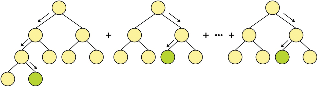
Figure 2: Structure of XGBoost

Also, XGBoost could automatically utilize the CPU multi-threaded parallel computing to accelerate the running speed. This feature signifies an enormous benefit of XGBoost over other approaches. XGBoost has considerably enhanced performance and effect. The XGBoost model can be expressed in the following:

y^i=∑m=1M fm(xi), fm∈F(21)

In Eq. (21), M indicates the number of trees, and F shows the elementary model of trees. The objective function can be described in Eq. (22):

L=∑i l(y^i,yi)+∑m Ω(fm)(22)

The error between the true and predicted values can be denoted as the loss function l, and the regularized function Ω for preventing over-fitting is determined in the following:

Ω(f)=γT+12λ‖w‖2(23)

In Eq. (23), all the trees’ weight and the number of leaves are indicated as w and T, correspondingly. Afterwards implementing the quadratic Taylor expansion on the objective function, the data gain produced afterwards every split of the objective function is formulated in the following:

Gain=12[(∑i∈ILgi)2∑i∈ILhi+λ+(∑i∈IRgi)2∑i∈IRhi+λ+(∑i∈Igi)2∑i∈Ihi+λ]−γ(24)

Note that the split threshold γ is added to Eq. (24) to prevent overfitting and inhibit the overgrowth of trees. Only if the data gain is better than γ is the leaf node allowable to split. Also, XGBoost has the following two features:

•   Splitting ends when the threshold is better than the weight of each sample on the leaf nodes to prevent the model from learning a special training sample.

•   The feature is sampled at random while building all the trees.

•   This feature could prevent the XGBoost module from over-fitting during the experiment.

4  Result Analysis

In this section, the insect classification results of the MMTL-IPCAC model are investigated on a dataset comprising 900 samples, as shown in Table 1. A few sample images are shown in Fig. 3.

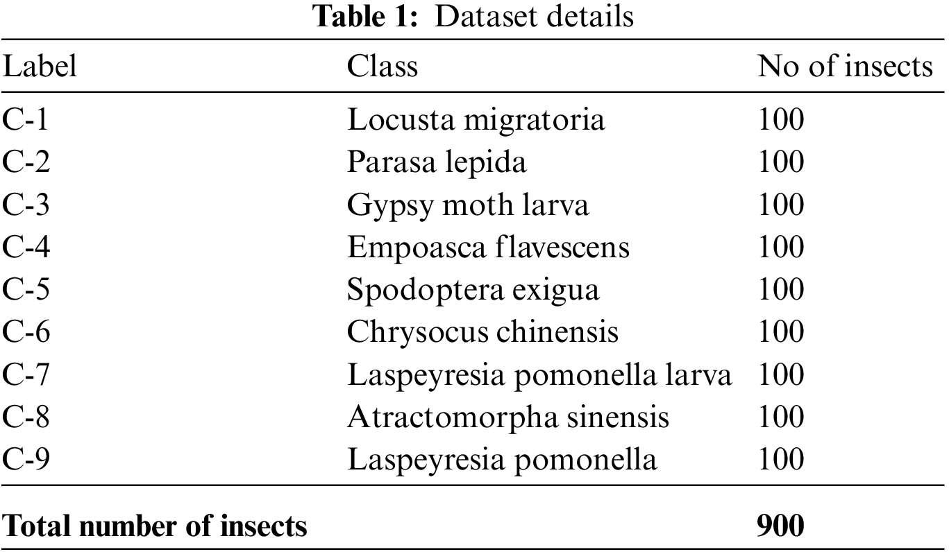
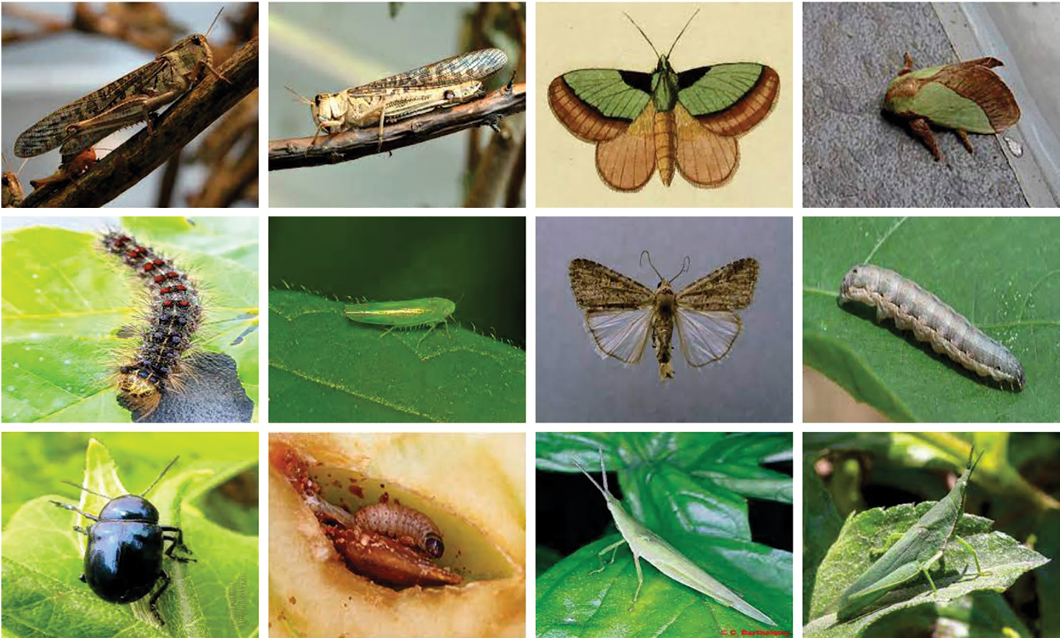
Figure 3: Sample images

The confusion matrices produced by the MMTL-IPCAC model on the applied dataset are given in Fig. 4. The figure implied that the MMTL-IPCAC model had enhanced performance on all the class labels.

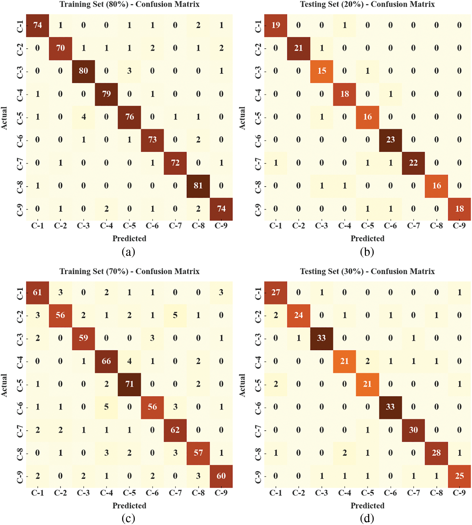
Figure 4: Confusion matrices of MMTL-IPCAC approach (a) 80% of TR data, (b) 20% of TS data, (c) 70% of TR data, and (d) 30% of TS data

Table 2 and Fig. 5 report the overall insect classification outcomes of the MMTL-IPCAC method on 80% of TR data and 20% of TS data. The simulation values reported the MMTL-IPCAC method had reported improved results under both classes. For example, with 80% of TR data and C1 class, the MMTL-IPCAC method gained average accuy, precn, recal, Fscore, and AUCscore of 98.75%, 96.10%, 92.50%, 94.27%, and 96.02% respectively. Similarly, and C2 class, the MMTL-IPCAC approach has attained average accuy, precn, recal, Fscore, and AUCscore of 98.47%, 95.89%, 89.74%, 92.72%, and 94.64%, correspondingly.

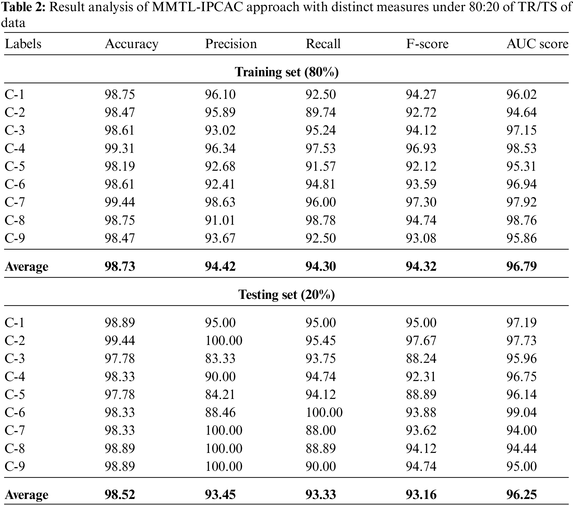
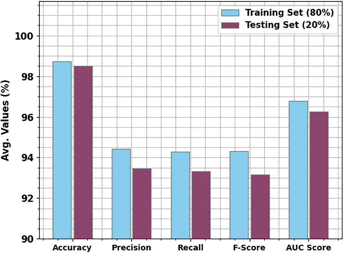
Figure 5: Average analysis of MMTL-IPCAC approach under 80:20 of TR/TS of data

Moreover, and C3 class, the MMTL-IPCAC approach has attained average accuy, precn, recal, Fscore, and AUCscore of 98.61%, 93.02%, 95.24%, 94.12%, and 97.15%, correspondingly. Furthermore, and the C4 class, the MMTL-IPCAC approach has attained average accuy, precn, recal, Fscore, and AUCscore of 99.31%, 96.34%, 97.53%, 96.93%, and 98.53% correspondingly. Also, and C5 class, the MMTL-IPCAC methodology has obtained average accuy, precn, recal, Fscore, and AUCscore of 98.19%, 92.68%, 91.57%, 92.12%, and 95.31%, correspondingly. Next, with 20% of TS data and C1 class, the MMTL-IPCAC method has acquired average accuy, precn, recal, Fscore, and AUCscore of 98.89%, 95%, 95%, 95%, and 97.19% correspondingly. Similarly, and the C2 class, the MMTL-IPCAC method has reached average accuy, precn, recal, Fscore, and AUCscore of 99.44%, 100%, 95.45%, 97.67%, and 97.73%, correspondingly. Besides, and C3 class, the MMTL-IPCAC methodology has attained average accuy, precn, recal, Fscore, and AUCscore of 97.78%, 83.33%, 93.75%, 88.24%, and 95.96%, correspondingly.

Table 3 and Fig. 6 report the overall insect classification outcomes of the MMTL-IPCAC method on 70% of TR data and 30% of TS data. The simulation values reported the MMTL-IPCAC approach had reported improved results under both classes. For example, with 70% of TR data and C1 class, the MMTL-IPCAC method has gained average accuy, precn, recal, Fscore, and AUCscore of 96.67%, 84.72%, 85.92%, 85.31%, and 91.97% correspondingly. Moreover, and C2 class, the MMTL-IPCAC approach has achieved average accuy, precn, recal, Fscore, and AUCscore of 96.51%, 88.89%, 78.87%, 83.58%, and 88.81%, correspondingly. Also, and C3 class, the MMTL-IPCAC technique has attained average accuy, precn, recal, Fscore, and AUCscore of 98.10%, 90.77%, 90.77%, 90.77%, and 94.85%, correspondingly. Furthermore, and the C4 class, the MMTL-IPCAC algorithm has attained average accuy, precn, recal, Fscore, and AUCscore of 96.35%, 81.48%, 89.19%, 85.16%, and 93.25%, correspondingly. Additionally, and the C5 class, the MMTL-IPCAC method has reached average accuy, precn, recal, Fscore, and AUCscore of 97.62%, 87.65%, 93.42%, 90.45%, and 95.81%, correspondingly.

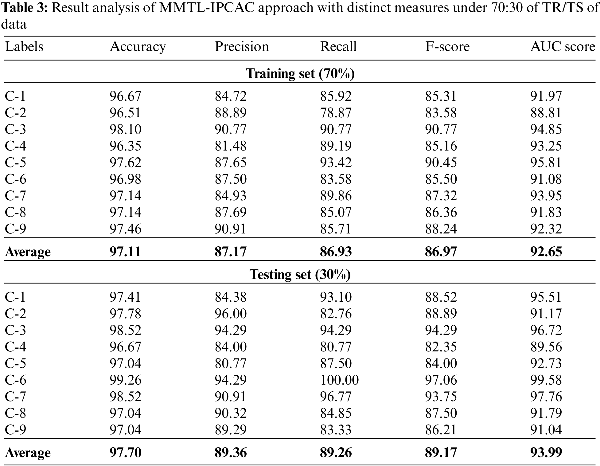
Figure 6: Average analysis of MMTL-IPCAC approach under 70:30 of TR/TS of data

Fig. 7 illustrates the TA and VA acquired by the AOHRD-BC2HI method on the 400X dataset. The figure emphasized that the AOHRD-BC2HI approach has reached higher values of TA and VA. The results denoted the TA is considered to be greater than the VA.

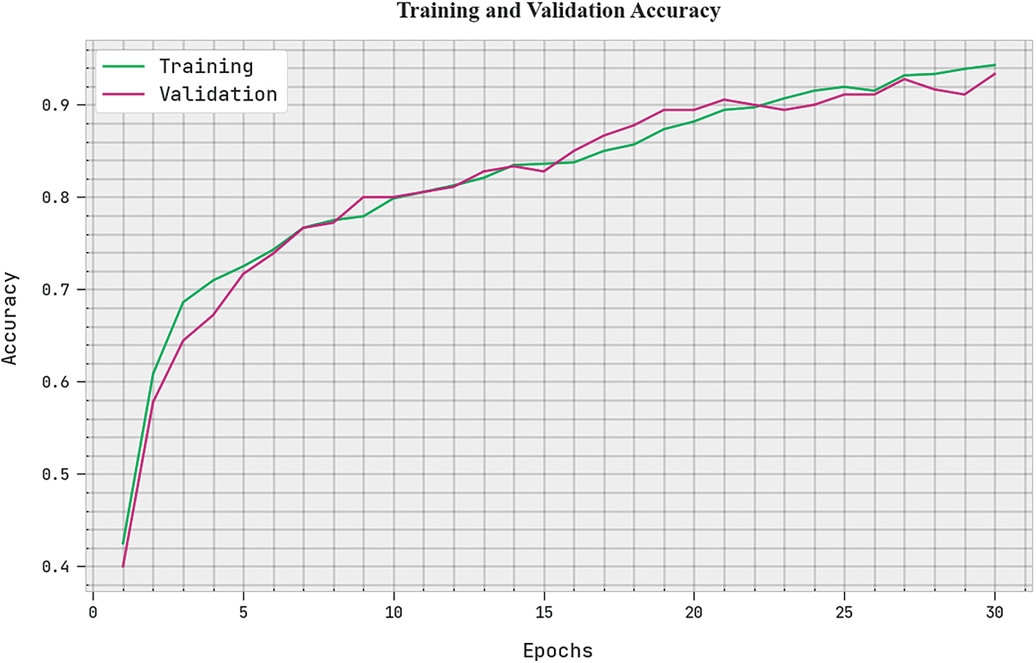
Figure 7: TA and VA analysis of the MMTL-IPCAC approach

Fig. 8 displays the TL and VL denoted by the AOHRD-BC2HI methodology on the 400X dataset. The figure showcases that the AOHRD-BC2HI approach has resulted in minimal values of TL and VL. These results ensured that the TL was lesser than the VL.

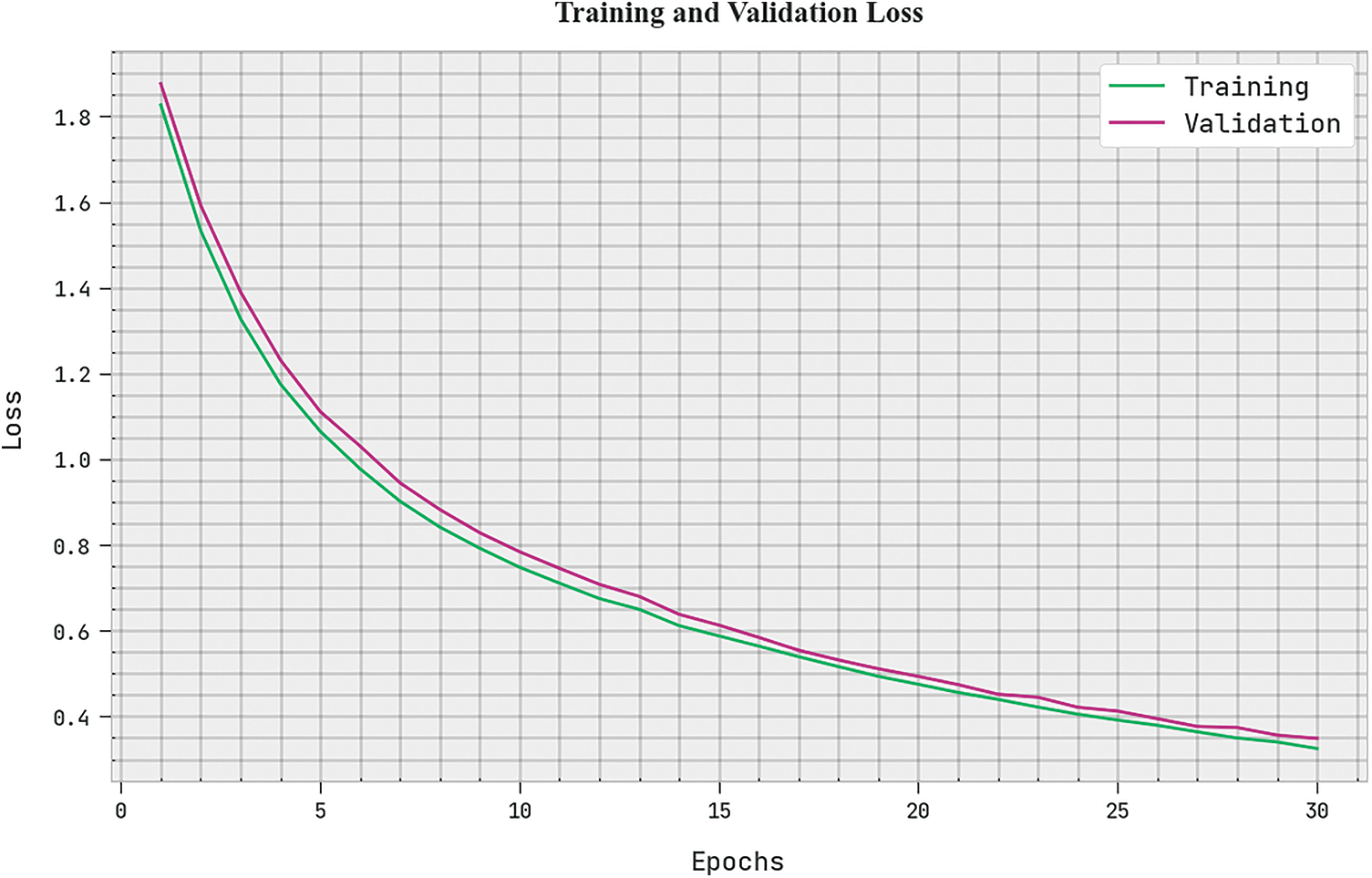
Figure 8: TL and VL analysis of the MMTL-IPCAC approach

The precision-recall values incurred by the MMTL-IPCAC model have demonstrated in Fig. 9. The figure represented that the MMTL-IPCAC method has properly categorized nine class labels and accomplished maximum precision-recall values.

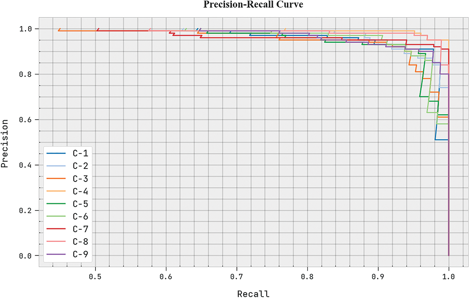
Figure 9: Precision-recall analysis of the MMTL-IPCAC approach

The ROC investigation of the MMTL-IPCAC method on the test data is demonstrated in Fig. 10. The figure exhibits the MMTL-IPCAC method has attained maximum ROC values under all classes.

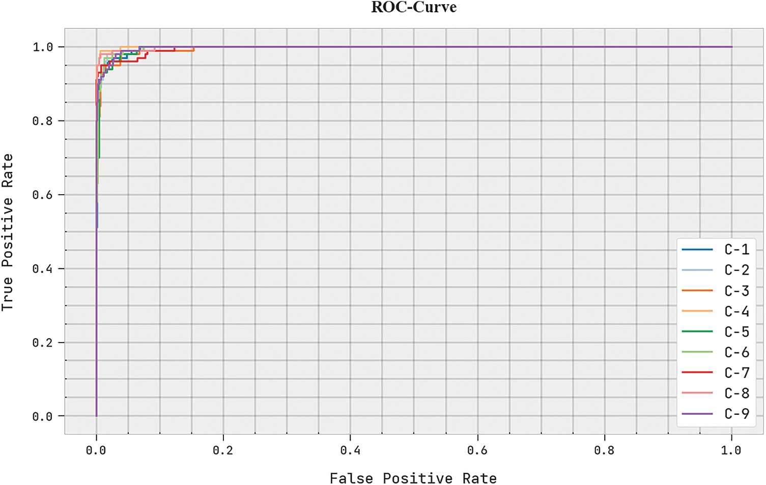
Figure 10: ROC curve analysis of the MMTL-IPCAC approach

To highlight the improved outcomes of the MMTL-IPCAC method, a wide-ranging experimental analysis is made in Table 4 and Fig. 11 [1]. These results implicit the ANN, SVM, and NB methods have shown poor classification outcomes over other models. Followed by the CNN and KNN models have reported moderately closer classification performance.

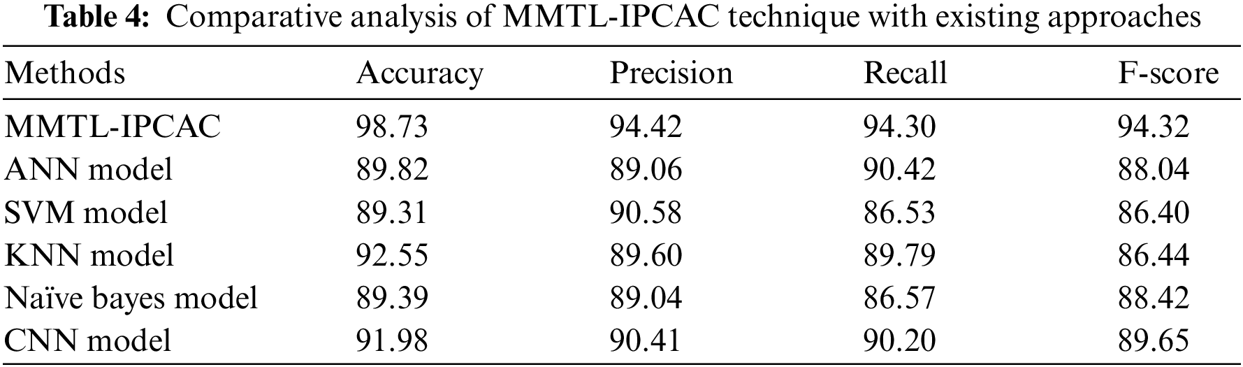
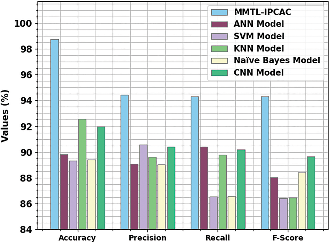
Figure 11: Comparative analysis of MMTL-IPCAC technique with existing methods

However, the experimental outcomes inferred that the MMTL-IPCAC model had shown enhanced results over other models with a maximum accuy of 98.73%. These results ensured that the MMTL-IPCAC model performed better on insert classification.

5  Conclusion

In this study, a new MMTL-IPCAC algorithm was developed for insect pest classification to improve agricultural pest control and crop productivity. Initially, the MMTL-IPCAC technique employed the CLAHE technique for image enhancement. The NASNet model is applied for feature extraction, and the MGWO algorithm is employed for the hyperparameter tuning process. At last, the XGBoost model is utilized to carry out the insect classification procedure. The simulation analysis of the MMTL-IPCAC technique can be tested on a benchmark dataset, and the results are scrutinized in distinct aspects. The comparison study stated the enhanced performance of the MMTL-IPCAC technique in the insect classification process. Thus, the MMTL-IPCAC technique can be employed for automated insect pest classification. In the future, hybrid DL methods will be applied to boost the insect classification efficacy of the presented MMTL-IPCAC method.

Funding Statement: Princess Nourah bint Abdulrahman University Researchers Supporting Project Number (PNURSP2023R384), Princess Nourah bint Abdulrahman University, Riyadh, Saudi Arabia.

Conflicts of Interest: The authors declare that they have no conflicts of interest to report regarding the present study.

References

1. T. Kasinathan, D. Singaraju and S. R. Uyyala, “Insect classification and detection in field crops using modern machine learning techniques,” Information Processing in Agriculture, vol. 8, no. 3, pp. 446–457, 2021. [Google Scholar]
2. J. B. Monis, R. Sarkar, S. N. Nagavarun and J. Bhadra, “Efficient Net: Identification of crop insects using convolutional neural networks,” in Int. Conf. on Advances in Computing, Communication and Applied Informatics (ACCAI), Chennai, India, pp. 1–7, 2022. [Google Scholar]
3. X. Wu, C. Zhan, Y. K. Lai, M. M. Cheng and J. Yang, “IP102: A large-scale benchmark dataset for insect pest recognition,” in Proc. of the IEEE/CVF Conf. on Computer Vision and Pattern Recognition, Long Beach, CA, USA, pp. 8787–8796, 2019. [Google Scholar]
4. K. Thenmozhi and U. S. Reddy, “Crop pest classification based on deep convolutional neural network and transfer learning,” Computers and Electronics in Agriculture, vol. 164, pp. 104906, 2019. [Google Scholar]
5. E. C. Tetila, B. B. Machado, G. V. Menezes, N. A. de Souza Belete, G. Astolfi et al., “A deep-learning approach for automatic counting of soybean insect pests,” IEEE Geoscience and Remote Sensing Letters, vol. 17, no. 10, pp. 1837–1841, 2019. [Google Scholar]
6. K. Bjerge, H. M. Mann and T. T. Høye, “Real-time insect tracking and monitoring with computer vision and deep learning,” Remote Sensing in Ecology and Conservation, vol. 8, no. 3, pp. 315–327, 2022. [Google Scholar]
7. J. G. A. Barbedo, “Detecting and classifying pests in crops using proximal images and machine learning: A review,” AI, vol. 1, no. 2, pp. 312–328, 2020. [Google Scholar]
8. M. C. F. Lima, M. E. D. de A. Leandro, C. Valero, L. C. P. Coronel and C. O. G. Bazzo, “Automatic detection and monitoring of insect pests—A review,” Agriculture, vol. 10, no. 5, pp. 161, 2020. [Google Scholar]
9. E. Ayan, H. Erbay and F. Varçın, “Crop pest classification with a genetic algorithm-based weighted ensemble of deep convolutional neural networks,” Computers and Electronics in Agriculture, vol. 179, pp. 105809, 2020. [Google Scholar]
10. A. Amrani, F. Sohel, D. Diepeveen, D. Murray and M. G. Jones, “Insect detection from imagery using YOLOv3-based adaptive feature fusion convolution network,” Crop and Pasture Science, 2022, https://doi.org/10.1071/CP21710 [Google Scholar] [CrossRef]
11. B. Ramalingam, R. E. Mohan, S. Pookkuttath, B. F. Gómez, C. S. C. S. Borusu et al. “Remote insects trap monitoring system using deep learning framework and IoT,” Sensors, vol. 20, no. 18, pp. 5280, 2020. [Google Scholar] [PubMed]
12. T. Kasinathan and S. R. Uyyala, “Machine learning ensemble with image processing for pest identification and classification in field crops,” Neural Computing and Applications, vol. 33, no. 13, pp. 7491–7504, 2021. [Google Scholar]
13. H. Li, S. Li, J. Yu, Y. Han and A. Dong, “Plant disease and insect pest identification based on vision transformer,” in Int. Conf. on Internet of Things and Machine Learning (IoTML 2021), Shanghai, China, vol. 12174, pp. 194–201, 2022. [Google Scholar]
14. Z. Shi, H. Dang, Z. Liu and X. Zhou, “Detection and identification of stored-grain insects using deep learning: A more effective neural network,” IEEE Access, vol. 8, pp. 163703–163714, 2020. [Google Scholar]
15. H. Kuzuhara, H. Takimoto, Y. Sato and A. Kanagawa, “Insect pest detection and identification method based on deep learning for realizing a pest control system,” in 59th Annual Conf. of the Society of Instrument and Control Engineers of Japan (SICE), Chiang Mai, Thailand, pp. 709–714, 2020. [Google Scholar]
16. H. X. Huynh, D. B. Lam, T. V. Ho, D. T. Le and L. M. Le, “CDNN model for insect classification based on deep neural network approach,” in Context-Aware Systems and Applications, and Nature of Computation and Communication, Lecture Notes of the Institute for Computer Sciences, Social Informatics and Telecommunications Engineering book series, vol. 298, pp. 127–142, Cham, My Tho City, Vietnam: Springer, 2019. https://doi.org/10.1007/978-3-030-34365-1_10 [Google Scholar] [CrossRef]
17. D. Xia, P. Chen, B. Wang, J. Zhang and C. Xie, “Insect detection and classification based on an improved convolutional neural network,” Sensors, vol. 18, no. 12, pp. 4169, 2018. [Google Scholar] [PubMed]
18. S. Sanagavarapu, S. Sridhar and T. V. Gopal, “COVID-19 identification in CLAHE enhanced CT scans with class imbalance using ensembled resnets,” in IEEE Int. IOT, Electronics and Mechatronics Conf. (IEMTRONICS), Toronto, ON, Canada, pp. 1–7, 2021. [Google Scholar]
19. K. Radhika, K. Devika, T. Aswathi, P. Sreevidya, V. Sowmya et al. “Performance analysis of NASNet on unconstrained ear recognition,” in Nature Inspired Computing for Data Science, Studies in Computational Intelligence book series, Cham, Springer, vol. 871, pp. 57–82, 2020. [Google Scholar]
20. M. Mehmood, N. Alshammari, S. A. Alanazi, A. Basharat, F. Ahmad et al. “Improved colorization and classification of intracranial tumor expanse in mri images via hybrid scheme of pix2pix-cgans and nasnet-large,” Journal of King Saud University-Computer and Information Sciences, vol. 164, pp. 104906, 2022. [Google Scholar]
21. S. Mirjalili, I. Aljarah, M. Mafarja, A. A. Heidari and H. Faris, “Grey wolf optimizer: Theory, literature review, and application in computational fluid dynamics problems,” Nature-Inspired Optimizers, Studies in Computational Intelligence book series, Cham, Springer, vol. 811, pp. 87–105, 2020. [Google Scholar]
22. M. A. Elaziz, A. Mabrouk, A. Dahou and S. A. Chelloug, “Medical image classification utilizing ensemble learning and levy flight-based honey badger algorithm on 6 g-enabled internet of things,” Computational Intelligence and Neuroscience, vol. 164, pp. 104906, 2022. [Google Scholar]
23. A. Ogunleye and Q. G. Wang, “XGBoost model for chronic kidney disease diagnosis,” IEEE/ACM Transactions on Computational Biology and Bioinformatics, vol. 17, no. 6, pp. 2131–2140, 2019. [Google Scholar]
Cite This Article
Copyright © 2023 The Author(s). Published by Tech Science Press.
This work is licensed under a Creative Commons Attribution 4.0 International License , which permits unrestricted use, distribution, and reproduction in any medium, provided the original work is properly cited.
Downloads
Citation Tools