A Novel Cluster Analysis-Based Crop Dataset Recommendation Method in Precision Farming

1  Introduction

Blockchain technology could revolutionize agriculture by addressing product fraud, traceability, price gouging, and consumer mistrust. The author [1] presented how blockchain technology can be used in agriculture to solve current problems by reviewing previous research and analyzing blockchain startup case studies. Blockchain makes possible a safer, better, more sustainable, and more reliable agri-food system. Agriculture and related industries are unquestionably the most important sources of income in rural India. Agriculture has a significant impact on the country’s GDP (GDP). The country is fortunate to have such a robust agricultural sector. Agriculture and related industries are by far the most significant sources of income in rural India. Agriculture significantly contributes to the country’s Gross Domestic Product (GDP) [2]. The country is fortunate to have a thriving agricultural industry. However, crop yield per hectare falls short of global standards. One of the reasons for the rise in suicides among India’s poor farmers could be this. However, agricultural production per hectare is low in comparison to global norms. This could be one of the reasons why so many small farmers have decided to relocate to India. Crop yield prediction is an important issue in the agricultural sector [3]. Every farmer’s goal is to understand their crop yield and whether or not it meets their goals based on their prior knowledge of that crop and yield prediction [4]. Crop yields are affected by pests, the environment, and harvesting procedures. It is necessary to have accurate crop history information to make decisions regarding managing agricultural risks [5].

Agriculture has a long tradition in India. India was recently ranked second in global agricultural output. For example, forestry and fisheries related to agriculture generated roughly half of all jobs and 16.6% of GDP in 2009. The agricultural sector’s contribution to India’s GDP is declining. Crop production is agriculture’s primary source of revenue [6,7]. Crop output is affected by various factors, including meteorological, geographic, organic, and economic considerations. Due to fluctuating market prices, farmers have difficulty deciding when and which crops to grow. According to Wikipedia [8], between 1.4% and 1.8% of 100,000 people in India committed suicide in the previous ten years. Farmers are unsure of what crop to plant, when to start, and where to plant it because of the unpredictable nature of the weather. Seasonal temperature variations and the accessibility of essential resources such as soil, water, and air call into question the use of various fertilizers. Crop yields are steadily declining in this situation. The problem can be solved by providing farmers with access to an intelligent, user-friendly recommendation system.

The majority of farmers in underdeveloped countries continue to employ centuries-old farming techniques. These methods do not ensure a high yield per acre. One of the numerous issues with conventional agriculture is that farmers choose crops based on market demand rather than the productivity of their land. Crop recommendation is a strategy that assists farmers in determining which crops will produce the most yields per hectare. A crop recommendation system, also known as a prediction system, is the art of anticipating crop yields to optimize productivity prior to harvesting. It is typically done several months in advance. Because crop recommendation systems entail processing vast amounts of soil, fertilizers, and geographical and meteorological data, machine learning (ML) approaches are utilized to handle this overwhelming data efficiently. ML-based systems can take many inputs and perform a range of non-linear tasks. They are comprehensive and cost-effective solutions for better crop advice and decision-making in general.

Programs that quantitatively explain plant-environment and soil feature interactions are used to provide crop recommendations. The technique starts with gathering a field soil sample for scientific soil testing. A field can be sampled so that the chemical composition of the soil sample, which is also influenced by temperature and rainfall, can precisely show the actual nutrient status of the field in a particular location, benefiting farmers and increasing production. This is the first fundamental premise of precision agriculture’s crop recommendation procedure for soil testing. B putting all this effort into the values and procedures, researchers can construct an intuitive crop recommendation system that delivers suggestions with a small margin of error depending on agricultural seasons and other parameters. This crop suggestion approach helps farmers make better-educated selections, resulting in more efficient and lucrative farming techniques.

From the literature, it is observed that most existing work needs to explain how and on what basis the crops were classified. They suggest crops based on soil properties or climatic conditions. If we only recommend using one of the two scenarios, the accuracy of the prediction decreases. We considered both scenarios in the proposed work to overcome the challenges above. This allows us to recommend the best dataset for the researchers, increasing the accuracy of crop recommendation.

Precision agriculture is essential in developing countries like India, where traditional or even ancient farming practices predominate. Precision agriculture, also known as site-specific agriculture, assists farmers in taking care of their land by increasing yield per unit of land and reducing pesticide and fertilizer waste. To classify yields by soil potential, statistical approaches are used. Farmers can harvest the right crops with management zones at the right sub-yields. This allows them to use less fertilizer, insecticide, and other inputs. Traditional yield prediction is based on a farmer’s previous crop harvesting at a specific time. Precision agriculture promotes yield prediction based on data. We use data mining, modeling, and statistical models to forecast crop harvest. Data-based yield estimates are getting closer to the actual crop yield. When selecting crops, many farmers overlook soil potential. The demand for “expert systems” is growing in tandem with the rise of Precision Agriculture. Precision agriculture, like other businesses, will increasingly rely on data. Using spatial data mining on the following datasets will become much more critical in the future and should be solved using intelligent informatics and geostatistics methods. Precision agriculture’s crop suggestion system can help farmers make better decisions. This technique chooses the best crops for a plot of land based on data and analytical models. This inspired us to conduct precision agriculture research.

The significant contributions of the paper are enlisted below.

•   The major challenge in the proposed work is the data. The data received from various sources is not in the proper format. The incorrect dataset format is transformed into the correct form by creating a data frame from all combinations of the supplied feature vectors.

•   Another finding is that numerical parameters such as N, P, K, and temperature have a discrete value range. It has been observed and tested that the most popular tree-based classification algorithms perform better with datasets that contain more categorical variables than numeric ones.

•   Recommendation of Crop Dataset using Cluster-based techniques.

•   The organization of the rest of the paper is as follows.

Section 2 discusses the background work of researchers in agriculture and yield prediction. Section 3 presents the proposed model for yield prediction and recommends which crop for cultivation. The model also suggests the best suitable time for the use of fertilizers. Section 4 discusses the results, and Section 5 concludes the paper.

2  Related Work

The authors of [9] predicted soybean yield in the United States using convolutional and recurrent neural networks. The MAPE of their model was 15% lower than that of typical remote sensing approaches (MAPE). Convolutional neural networks can predict crop yields using satellite images [10]. Their model outperformed other machine learning approaches and employed three-dimensional convolution to incorporate spatial and time variables. One of the most challenging problems in precision agriculture is predicting crop production, and numerous working models have been suggested and demonstrated. Because crop production is controlled by various factors, including soil, weather, fertilizer application rate, and seed type, this challenge needs the usage of several datasets [11].

The work published in [12] offered a crop recommendation method based on machine learning. The dataset included temperature, humidity, average rainfall, soil pH, nitrogen, potassium, and phosphorus requirements, which the authors used to train machine learning models. In terms of accuracy, the Nave Bayes classifier performed admirably. However, after tweaking the hyperparameters, the Random Forest classifier performs better and is considered for prediction. The algorithm forecasts the top five crops that can be cultivated in the current location. The soil, climate, and geographical factors influence crop prediction for a specific location.

The authors of [13] used feature selection techniques such as Recursive Feature Elimination (RFE), Boruta, and Sequential Forward Feature Selection (SFFS) on the dataset to select precise soil and environmental characteristics for crop prediction. The RFE method determines the most precise features. Furthermore, when RFE is used in conjunction with a bagging classifier, the accuracy of crop prediction based on soil and environmental characteristics improves.

The dataset contains 135 different crops in the target column that were grown in the corresponding location in India, according to the authors of [14]. According to the authors, the K Nearest Neighbor model accurately predicts the type of crop cultivated at the location. The authors of [15] created a model for Maharashtra state that helps farmers decide which crop to cultivate based on crop productivity using a multilayer perceptron neural network. The predicted model recommends crops based on the district and weather. Using the Adam optimizer, the anticipated model performs with 90% accuracy.

The authors of [16] presented a mobile application for a user who inputs soil type and area as input and estimates crop yield per hectare for the states of Karnataka and Maharashtra. In addition, the model predicts agricultural output per hectare for a chosen crop. According to the authors, Random Forest produces the best results, with 95% accuracy. The proposed approach also recommends the optimal fertilizer application time to maximize crop output. Farmers frequently require an intelligent system to select a crop that maximizes crop output. The authors of [17] addressed this issue using Machine Learning approaches. The proposed models indicate a crop planting order for the season. Some farmers want crop yield information to sow crops in the future. Researchers in [18] tackled this novelty by employing advanced regression techniques and improving the model’s performance by stacking regression.

Using data analytics, researchers in [19] examined a massive agricultural data collection to provide meaningful information. We used K-Means and the Apriori technique to investigate the data’s qualities. In addition, the authors devised a Nave Bayes model to predict crop name and yield. The authors of [20] employed a Random Forest regression model to forecast crop yield per hectare using data from the Indian government, such as rainfall, temperature, season, and area. Only some crops satisfy farmers regarding crop yield and choices for a specific season. The authors of [21] presented a software solution named ‘Crop Advisor,’ which will serve as a user-friendly application for farmers to learn about the climate parameters influencing crop yields in Madhya Pradesh. The authors employed the C4.5 method to determine the most influential climatic parameters.

The authors of [22] offered various machine learning regression algorithms based on geological and climatic factors to forecast the highest crop yields among rice, ragi, gramme, potato, and onion. To improve accuracy, the majority voting method was used. The authors of [23] suggested a decision tree technique for predicting crop output in Karnataka state based on soil, planting, harvesting, and season data. The authors stated that clustering and classification techniques might be coupled to achieve superior results. The authors of [24] suggested a strategy for predicting the best crop for high yield before deciding whether or not to cultivate the crop for the farmer. The authors employed various boosting regression techniques. XGB regression with hyper-parameter tuning outperformed other models in terms of RMSE.

The author [25] selects and discusses ML and DM datasets that academics utilize for Internet anomaly traffic classification research. A short ML/DM tutorial on Internet traffic classification with a feature dataset is provided for better comprehension. Read and summarized the most important and commonly cited methodologies and feature datasets. Because data is vital in Internet traffic classification using the ML/DM technique, various well-known and widely used datasets with detailed statistical properties are also provided.

Recently the author [26] presented a hybrid recommendation algorithms model for short-term and long-term behavior; however, they are static and need help discovering relationships between behaviors and objects. These algorithms also ignore location-based data when providing recommendations. The research proposes a hybrid location-centric prediction (HLCP) model that accounts for users’ dynamic behavior to overcome the issues. HLCP efficiently learns short-term and long-term contexts using Feed Forward Neural Networks and Recurrent Neural Networks.

This study improved a genetic algorithm (IGA) for recommending crop nutrition levels. The algorithm optimizes by exploring and exploiting the neighborhood. The model improved local optimization in population strategy to avoid premature local individuals. Diversity preserves population knowledge. In real-world datasets, the novel IGA method may outperform conventional recommendations. As a result, the program optimizes production and nutrient levels [27].

The end-to-end multi-objective neural evolutionary algorithm (MONEADD) for combinatorial optimization is introduced in this study. It is governed by decomposition and supremacy. MONEADD is an end-to-end approach that uses genetic processes and incentive signals to grow neural networks for combinatorial optimization tasks. Each generation retains non-dominated neural networks based on dominance and decomposition to accelerate convergence. Traditional heuristic approaches start from scratch for each test problem, whereas the trained model can answer equivalent questions during inference. Three multi-objective search strategies improve model inference performance [28].

3  Materials and Methods

3.1 Dataset Overview and Data Collection

The research was carried out in the state of Karnataka, India. The analysis examines eight variables for various crops. The minimum amounts of fertilizer required are nitrogen (N), phosphorus (P), and potassium (K). Another parameter used in the study is pH. Soil pH is a measure of the soil’s acidity or alkalinity. The other four parameters for increased crop productivity are temperature, rainfall conditions, soil type, and season, as shown in Table 1.

3.2 Datasets Construction

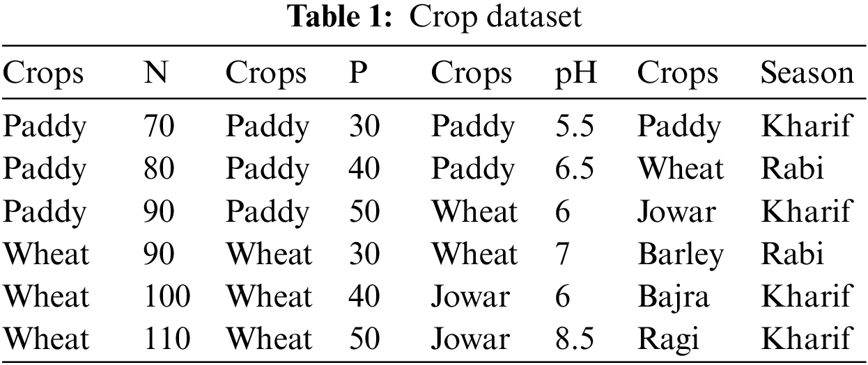
Table 1 demonstrates that the collected data needs to be in the correct format. The incorrect dataset format is translated into the right format by generating a data frame from all combinations of the supplied feature vectors [29]. Another discovery is that numerical parameters like N, P, K, and temperature have discrete value ranges. The bulk of prominent tree-based classification algorithms has been seen and tested to perform better with datasets that contain more categorical variables than numeric ones. The gathered data is processed in this context to turn its discrete numeric vectors into category vectors. As a result, we have two datasets: one with many numerical variables and one with many categorical variables. Tables 2 and 3 display these datasets.

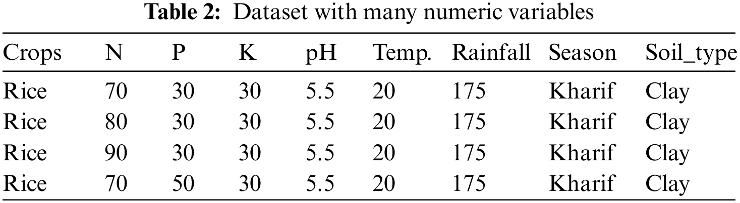
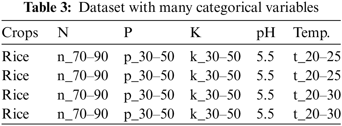
Fig. 1 depicts an abstract representation of the entire dataset construction process. Because our initial datasets are mixed, we will use an extension to the K-means algorithm, i.e., k-prototypes clustering, as well as two heuristic methods, factor, and numeric methods, to generate new datasets in addition to the class memberships.

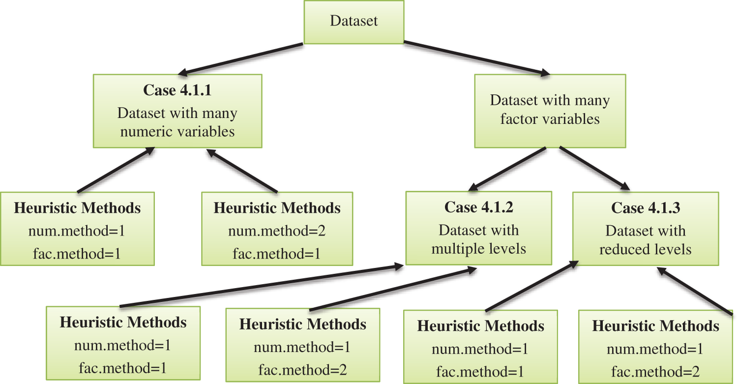
Figure 1: An overview of dataset construction

Case 4.1.1 illustrates a dataset with many numeric variables on which the heuristic method is used to build a new dataset with both numeric and factor values set to “1,” as illustrated in Fig. 1. Case 4.1.1 also undergoes another heuristic iteration, this time with the numeric method set to “2” and the factor method set to “1.”

Case 4.1.1 represents a dataset with many numeric variables, but Case 4.1.2 and Case 4.1.3 are characterized by a dataset with multiple factor variables. Case 4.1.2 represents multi-level datasets and separates them into two heuristic iterations, one with numeric and factor methods set to “1” and the other with numeric and factor methods set to “1” and “2,” respectively. Case 4.0.3, on the other hand, works with a reduced-level dataset. It also makes use of a heuristic method with two integer value possibilities. We finally have six datasets, two for each example.

3.3 Algorithm for Crop Recommendation

Input: D: Crop dataset containing n instances.

Output: The output is a class membership with the object assigned to the class based on the variables’ lambda estimate.

1 ds: = loadDataset ();

2 Apply standard preprocessing on the dataset;

3 if! target membership then

4   if ds is of mixed type, then

5    if numeric discrete-valued attributes, then

6      transform to factors;

7      ds:= generateDataset ();

8     end

9     if factor attributes have many levels, then

10       group them accordingly based on domain knowledge;

11       ds := generateDataset ();

12     end

13     for each outcome D of datasets do

14       // over the range to estimate the best k;

15       kbest := clusterValidation ();

16       // Investigate the variable’s variance and concentration;

17       lmd := lambdaEst ();

18       // Run the kproto function with kbest and lambda;

19       kpres := partition (ds, kbest, lmd);

20       ds := generateDataset ();

21     end

22    end

23 end

24 Update the cluster numbers at the end to the new datasets as target classes.

The algorithm shows how to create mixed-type datasets based on soil properties, season, rainfall, and temperature. The algorithm receives data partition (parameter D) as input, which represents the entire set of training tuples with excluded class labels (shown in line no. 3). The algorithm generates a class membership model in which objects are assigned to the class based on a lambda estimate [30].

The procedure begins with standard data preprocessing, such as variable normalization, discrete numeric to-factor conversion, and level reduction. The algorithm computes k-prototypes clustering for diverse datasets, shown in lines 13 to 20. K-prototyping is a modified version of the k-Means algorithm used to create clusters of large datasets with categorical values, recomputed cluster prototypes through iterations, and reassign clusters.

Equation d(x,y=deuclid(x,y)+λsimpleMatching(x,y) is used to assign clusters.

Heuristic methods are used for the computation of cluster prototypes as cluster means for numeric variables (standard deviation (num_method:= 2) or Variance (num_method:= 1)) and modes for factors

(1−∑ipi2(facMethod=1)) or (1−maxipi(facMethod=2)) is calculated.

The algorithm calls clusterValidation ( ) for each dataset retrieved for partitioning from lines 7 and 11. The preferred validation index is calculated using the following function:

McClain

McClain=Sw_Sb(1)

Sw Represents the total sum of within-cluster distances divided by the number of individuals’ within-cluster distances. On the other hand, Sb is the total sum of between-cluster distances divided by the total number of individuals between-cluster distances. The minimum value of the index denotes the optimal number of cluster silhouette.

We make use of the McClain and Silhouette clusters as our optimization model. A method for analyzing and confirming consistency within data clusters is the silhouette method. The method gives a clear graphic representation of each object’s classification accuracy. The silhouette value contrasts an object’s separation from other clusters with its cohesion with its own cluster. We can directly optimize the silhouette instead of using the average silhouette to evaluate a clustering from k-medoids or k-means. These methods assign points to the closest cluster, which is best.

Silhouette=1n∑i=1nb(i)−a(i)max(a(i),b(i))(2)

The average dissimilarity of the ith object to all other objects in the same cluster is given by a(i). b(i) = min(d(i, C)), where d(i, C) is the mean dissimilarity of the ith object to all other objects other than those in the same cluster. In the meantime, the maximum index value indicates the optimal number of groups [30]. In the end, the clusters generated from the above computation are tagged to every dataset accordingly as target classes in line no. 24 of the algorithm. We use the Silhouette and McClain clusters as an optimization model to determine the optimal number of clusters.

4  Results and Discussions

The dataset used for the experimental analysis is of mixed type (numeric and categorical). To achieve a better balance between the Euclidean distance of numeric variables and the simple matching coefficient of categorical variables, the optimal value of lambda is estimated to investigate the variables’ variance for k-prototype clustering. To accomplish this, we used lambda as a metric. The same explanation is given in all three cases. The initial crop dataset contains no class labels (presented in Table 1). Before proceeding with the rest of the calculation, we must establish class labels because these are essential for decision tree-based models to categorize and classify the crops. We employ a mixed-type partitioning method to produce class labels for each crop. The data input for the function included two-factor variables—soil type and season—as well as six numerical variables—annual rainfall, pH, temperature, Nitrogen (N), Phosphorus (P), and Potassium (K). The number of observations that belong to each cluster is one of the simplest ways to determine the usefulness of a cluster set. The McClain and silhouette equations are used to calculate the optimal value of k for a balanced cluster. It is critical to note that extreme cluster sizes are unlikely to be helpful.

4.1 Case 1: Dataset with Many Numeric Variables

Along with an explanation of the dataset’s actual contents, Fig. 2 provides a primitive overview of the data format in terms of observations (rows) and variables (columns). There are 44,280 observations of 9 different variables in the data frame [31].

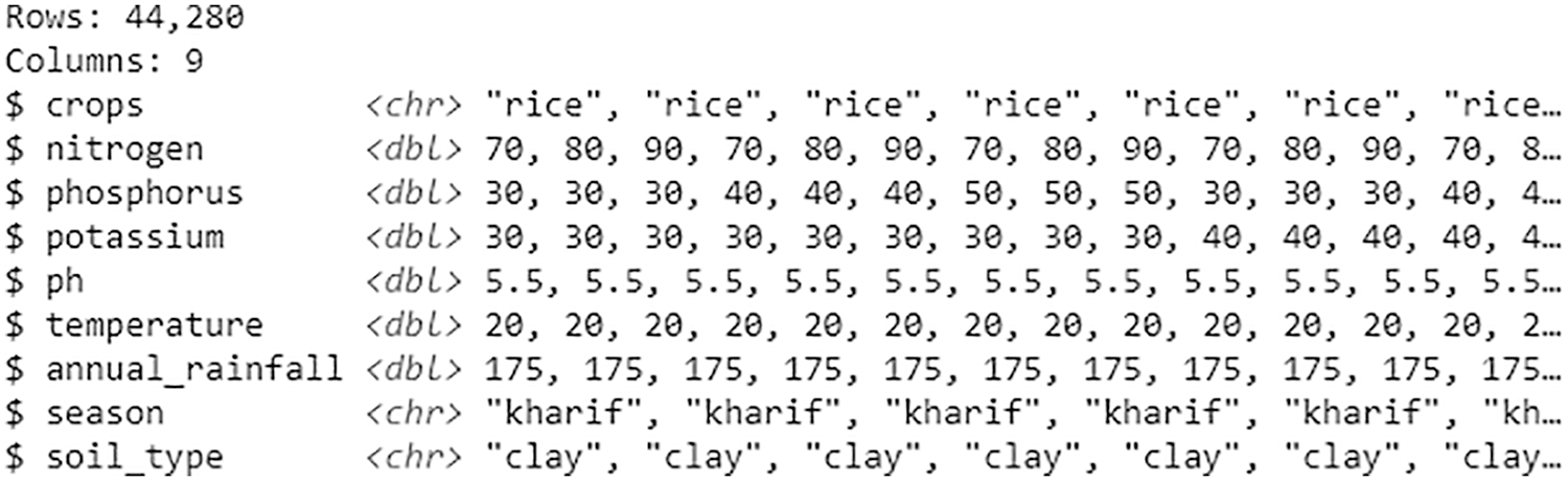
Figure 2: Dataset with many numeric variables

The below Fig. 3 illustrates the results obtained after plotting the balanced cluster using the Silhouette criterion, which identified 17 clusters. As the dataset is of mixed type, a better balance is achieved between the Euclidean distance of numeric variables and the simple matching coefficient between categorical variables. The optimal value of lambda is estimated to investigate the variables’ variance/concentrations for k-prototype clustering. The “clustMixType” is a tool used during the implementation process, which provides an implementation of k-prototypes in R. It computes k-prototypes clustering for mixed-type data. An implementation of the k-prototypes algorithm is given by the function

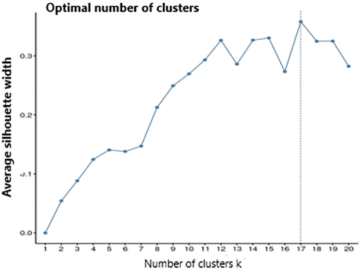
Figure 3: Plot of the ASW indices for 1–20 clusters. The function of lambda estimation supports and works with two heuristic methods

kproto(x, k, lambda = NULL, iter.max = 100, nstart = 1, na.rm = TRUE)

•   Numeric method

•   Factor method

We use lambda > than zero, to balance the simple matching coefficient between categorical variables and Euclidean distance between numerical variables. The order of a vector variable-specific factor must match the data variables. All variable distances are multiplied by lambda values.

Case 4.1.1-Task 1: Case 4.1.1’s dataset contains more numerical variables, so the numeric method with the integer value “1” and the factor method with the letter “1” is used. The clusters are then created based on the previously provided parameter values.

Fig. 4 demonstrates the process of k-prototype clustering’s object return, which contains a series of useful information.

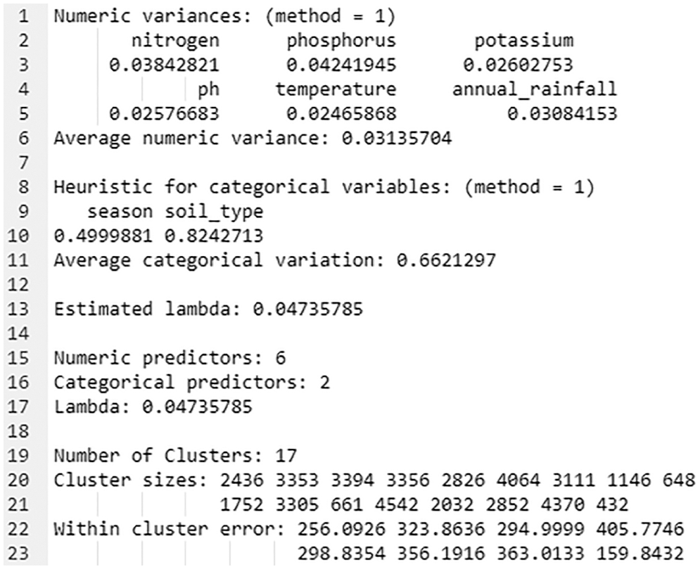
Figure 4: kproto() object of numc_method 1

The output of a function is a list with four components. Using Eq. (3), Lambda is calculated using heuristic approaches with the ratio of all numeric/factor variable means.

λ=averagenumericvariancesaveragecategoricalvariation=0.03135700.6621297=0.04735785(3)

Cluster returns the number of formed clusters (i.e., 17), whereas Cluster sizes return the number of instances in each group for the given dataset with 6 numeric and 2 categorical attributes. The best lambda value found is = 0.04735785 (as depicted in line no. 17 of Fig. 4). The values in lines 20 and 21 identify several instances that belong to clusters 1, 2, 3, and so on (such as 2436, 3353, 3394, etc.). The within-cluster-error function returns the error rate for each cluster.

The results of the k-prototypes clustering for cluster interpretation are shown in Figs. 5 and 6. The number of clusters is represented on the x-axis, the scaled range of attribute values is represented on the y-axis, and box plots and bar plots of each cluster are generated, and presented below for categorical and numerical variables.

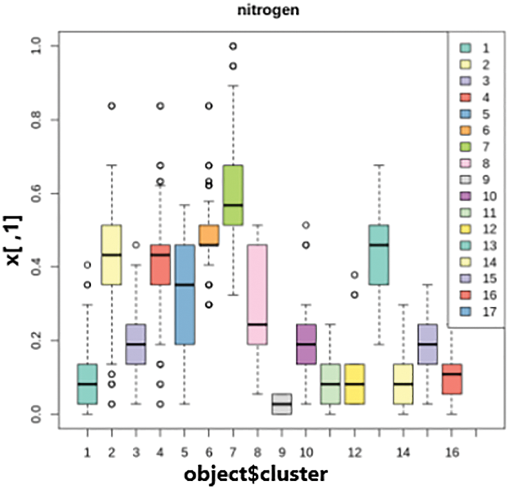
Figure 5: Cluster interpretations of nitrogen

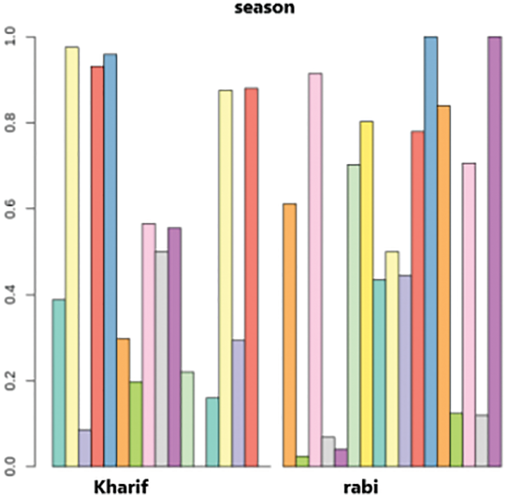
Figure 6: Cluster interpretations of season

Based on the above cluster interpretations, it is possible to conclude that observations/readings from one cluster differ considerably from those from other clusters. Consider an example as shown in Fig. 6, it is noticed that the first cluster in the kharif season has a value of 0.4. In contrast, the first rabi season cluster has a value of 0.6. Furthermore, the rabi season’s final cluster has a value of 1.0, whereas the kharif season’s last cluster has no value. So, it follows that the clusters created during the kharif season have values that are entirely different from those during the rabi season. The resulting cluster numbers are prepended with the word class as a result of class labels shown in Fig. 7.

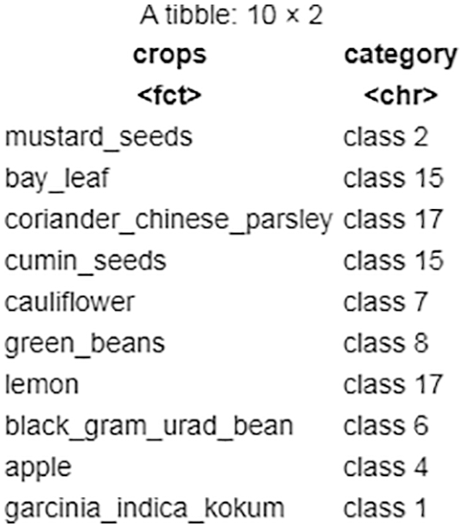
Figure 7: A quick sanity check of task 1 clusters

Case 4.1.1-Task 2: For the same dataset in Case 4.1.1, the integer values “2” and “1” are applied to form different sets of clusters. The explanation from Fig. 4 is applied again here to obtain the optimal lambda value for creating the same clusters.

λ=averagenumericstandarddeviationaveragecategoricalvariation=0.17608170.6621297=0.2659323(4)

The obtained λ value along with the above-assigned parameter values; the resulting cluster numbers are tagged with class labels and furnished in Fig. 8. Based on the tasks performed on the dataset (Case 4.1.1), the majority of the variables are numeric, with only two being categorical. Integer value has little effect on cluster formation when the factor method is changed.

Figure 8: A quick sanity check of task 2 clusters

4.2 Case 2: Dataset with Many Categorical Variables

The below Fig. 9 depicts the basic data shape in terms of observations (rows) and variables (columns), as well as a summary of the dataset’s actual contents. The data set contains 1,904 observations across 9 variables.

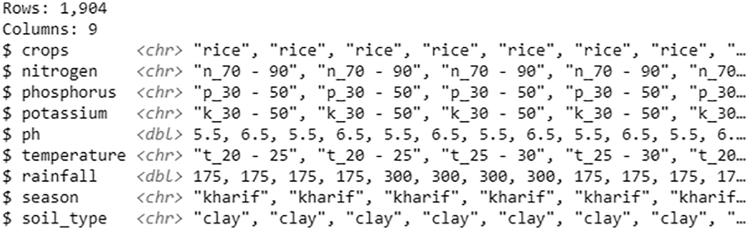
Figure 9: Dataset with many categorical variables

The issues in the dataset are factors that have multi-levels [31]. Depending on the circumstances, these variables can be ignored. In this instance, we identified and presented them in Fig. 10.

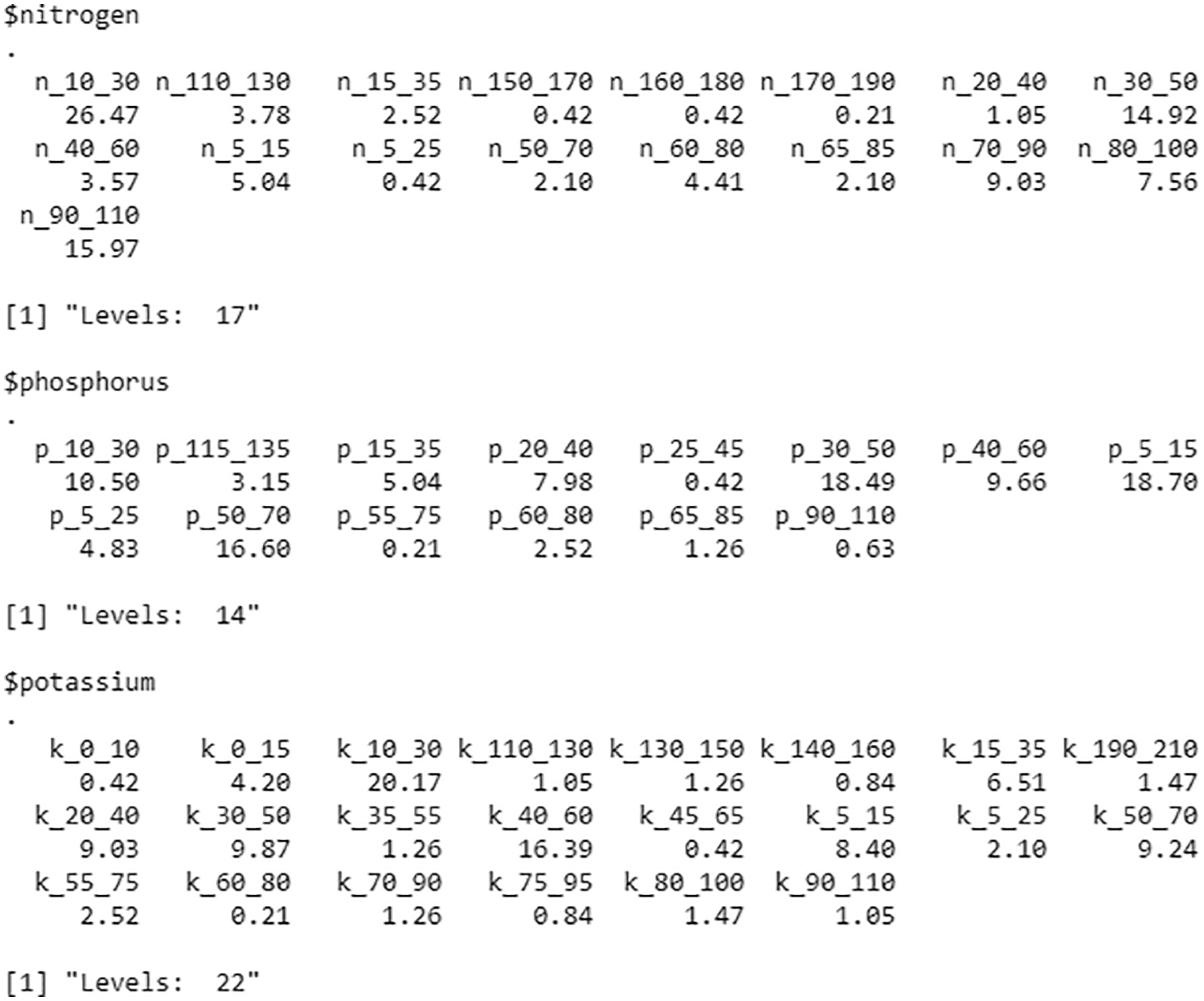
Figure 10: Distribution of observations across levels

The process to generate class labels for crop dataset: The crop data class labels are generated using the same procedure as in Case 4.1.1. Nitrogen (N), Phosphorus (P), Potassium (K), temperature, season, soil type, and two numeric variables pH and rainfall are the factor variables employed here.

Fig. 11 depicts the results of plotting the silhouette and McClain criteria with the vector specifying the search range [10:20] for the optimum number of clusters and repetitive computations with random initialization of 5. They pick up 20 clusters.

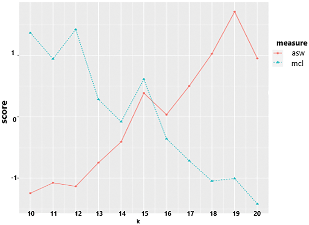
Figure 11: Plot b/w ASW and McClain indices

Case 4.1.2-Task 1: There are more factor variables in the dataset representing Case 4.1.2. As a result, with integer value 1, the numeric and factor methods are used. As shown in Section 4.1 (Fig. 4), the lambda value is obtained for the resultant object using Eq. (5). The value obtained from Eq. (5) aids in the formation of distinct clusters.

λ=averagenumericvarianceaveragecategoricalvariation=0.0330.792=0.04(5)

Figs. 12 and 13 represents the visualization of the result of k-prototypes clustering for cluster interpretation of pH and Season. Fig. 13 depicts the first cluster in the kharif season has a value of 0.3. On the other hand, the first cluster in the Rabi season has a value of 0.8. Furthermore, kharif last cluster is in the range of 0.8–0.9, whereas Rabi’s last cluster is 0.1. So, it follows that the clusters created during the kharif season have values that are entirely different from those during the rabi season.

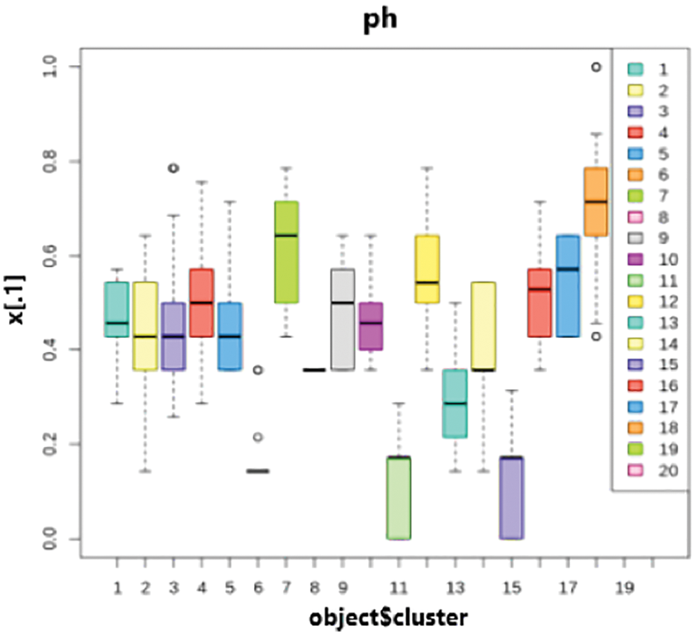
Figure 12: Cluster interpretations of pH

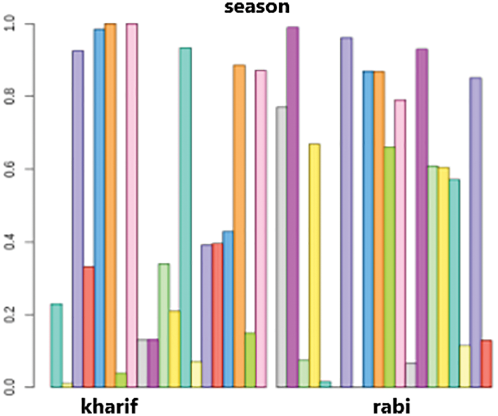
Figure 13: Cluster interpretations of season

With the above-mentioned parameter values, the resulting cluster numbers are prepended with the word class as shown in Fig. 14.

Figure 14: Task 1-sanity check of clustering

Case 4.1.2-Task 2: in Case 4.1.2, the integer values “1” and “2” are used to form different sets of clusters for the same dataset. As shown in Fig. 4 the resultant object gives the lambda value shown in Eq. (6), which aids in forming precise clusters.

λ=averagenumericvarianceaveragecategoricalvariation=0.0330.712=0.05(6)

The resulting cluster numbers are prepended with the word class using the above-mentioned parameter values, as shown in Fig. 15. The majority of the variables in the dataset are categorical, with only two being numeric, according to the task performed on the dataset (Case 4.1.2). When the numeric method is varied, integer value has little effect on cluster formation.

Figure 15: Task 2-sanity check of clustering

4.3 Case 3: Dataset Featuring Reduced Level of Many Categorical Variables

From Fig. 10 it is observed that in Case 4.1.2 dataset has categorical variables with many levels. The multitudes of groups present in every single attribute make the application of tree-based models for retrieving required information a time-consuming process [32].

To cut down the computation time when dealing with the overwhelming levels, we have made a group of nearer values while keeping the margin of ±10 while simultaneously ensuring that our results remain impartial. Fig. 16 shows a dataset that features nine variables with a total of 1,904 observations of reduced levels.

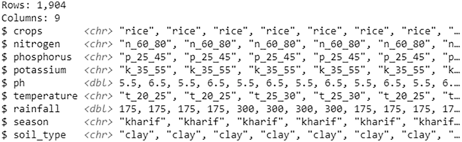
Figure 16: Dataset with many categorical variables

Case 4.1.3-Task 1:

In Fig. 17, the distribution of each variable is illustrated. If we observe Fig. 17 and compare it to the levels shown in Fig. 10, we can quickly tell that the sizes of the levels are trimmed down by half. Moreover, crop data’s class labels are formed similarly to Case 4.1.2 with fewer factor levels of the dataset. Lastly, 20 clusters are picked up by the criteria (McClain and Silhouette), and they are generated by employing the similar process used for the Task 1 of Case 4.1.2.

Figure 17: Distribution of observations across levels for case 3

Visualization of k-prototypes clustering results for cluster interpretation of pH and Season is presented in Figs. 18 and 19. Fig. 19 represents that the first cluster in the Kharif season gets a value in the range of 0.6 and 0.8. On the other hand, the first cluster in the Rabi season has a value range of 0.2 and 0.4. Moreover, Kharif’s last group is in the range of 0.0–0.2; the last cluster of Rabi gets approximately 1.0.

Figure 18: Cluster interpretations of pH

Figure 19: Cluster interpretations of season

According to Fig. 4 from Section 4.1 the lambda value is obtained through the resultant object. This value, as shown in Eq. (7), helps to form precise clusters.

λ=averagenumericvarianceaveragecategoricalvariation=0.030.72=0.05(7)

With the above-assigned parameter values and λ, the resulting cluster numbers are tagged with world-class due to class labels shown in Fig. 20.

Figure 20: Task 1-sanity check of clustering

Case 4.1.3-Task 2: Further, the integer values “1” and “2” are used for the same dataset in Task 1 to create different sets of clusters. Going by Fig. 4 explanation, the lambda value is obtained through the resultant object. As shown in Eq. (8), this value assists in forming precise clusters.

λ=averagenumericvarianceaveragecategoricalvariation=0.030.63=0.05(8)

With the above-assigned parameter values and λ, the resulting cluster numbers are prepended with the word class due to class labels shown in Fig. 21.

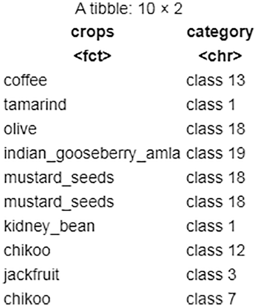
Figure 21: Task 2-sanity check of clustering

The observation of the tasks performed on the Case 4.1.3 dataset suggests that all variables are categorical except for two numeric ones. The variation of the numeric method integer value doesn’t significantly affect the formation of clusters. In the last, if we observe Figs. 6, 13, and 19, we can easily conclude that the clusters in the Kharif season present entirely different values than what we found out with the clusters of the Rabi season. It is essential to mention here that the inference mentioned above reveals that the clusters are appropriately created. Moreover, datasets representing all the cases discussed in the above study feature some outliers in some clusters. Fig. 5 of Case 4.1.1, Fig. 12 of Case 4.1.2, and Fig. 18 of Case 4.1.3 show those outliers. It is worth mentioning that there is a way to cut down the error rate value, i.e., fine-tuning the lambda value. However, we did not fine-tune the lambda value in this study because the clusters obtained in every case are too large or small. This disparity in the cluster values renders the observations not very useful for further proceeding of the study. In short, fine-tuning the lambda value would only amount to overwork for the given datasets without offering any valuable input.

5  Conclusion

Data mining and analytics involve evaluating and modeling data to draw conclusions and enhance decision-making. Precision agriculture uses advanced data mining tools to advance agriculture. Lack of farm management knowledge prevents selecting suitable datasets and crops for certain agro-fields. The cluster analysis performed by the algorithm iteration for the dataset with numeric variables reveals that values in one cluster differ significantly from values in other clusters. In addition, except for two categorical variables, the majority of variables in the same example are numerical. This means that changing the factor method’s integer value has no discernible effect on cluster formation. Case 2 draws the same conclusion as the first: all variables are numeric, but two and the factor method integer values are not closely related to cluster formation. The third case, with a dataset of reduced levels of many categorical variables, also reveals a value difference between clusters. The research’s overall findings can be divided into three categories. Clusters differ significantly between the Kharif and Rabi seasons. The vast majority of variables are categorical in nature rather than numerical. The integral value of the numerical approach has little effect on cluster formation.

Acknowledgement: The authors would like to thank Bapuji Institute of Engineering and Technology for providing the resources for this research. The authors extend their appreciation to the Deputyship for Research & Innovation, Ministry of Education in Saudi Arabia, for funding this research work through project number IF_2020_NBU_322.

Funding Statement: This research work was funded by the Institutional Fund Projects under Grant No. (IFPIP: 959-611-1443). The authors gratefully acknowledge the technical and financial support provided by the Ministry of Education and King Abdulaziz University, DSR, Jeddah, Saudi Arabia.

Conflicts of Interest:: The authors declare that they have no conflicts of interest to report regarding the present study.

References

1. S. Umamaheswari, S. Sreeram, N. Kritika and D. R. J. Prasanth, “Biot: Blockchain-based IoT for agriculture,” in 2019 11th Int. Conf. on Advanced Computing (ICoAC), Chennai, India, vol. 1, pp. 324–327, 2019. [Google Scholar]
2. A. Jain, “Analysis of growth and instability in the area, production, yield, and price of rice in India,” Journal of Social Change and Development, vol. 15, no. 2, pp. 46–66, 2018. [Google Scholar]
3. E. Manjula and S. Djodiltachoumy, “A model for prediction of crop yield,” International Journal of Computational Intelligence and Informatics, vol. 6, no. 4, pp. 298–305, 2017. [Google Scholar]
4. B. M. Sagar and N. K. Cauvery, “Agriculture data analytics in crop yield estimation: A critical review,” Indonesian Journal of Electrical Engineering and Computer Science, vol. 12, no. 3, pp. 1087–1093, 2018. [Google Scholar]
5. S. Wolfert, L. Ge, C. Verdouw and M. J. Bogaardt, “Big data in smart farming–A review,” Agricultural Systems, vol. 153, pp. 69–80, 2017. [Google Scholar]
6. J. W. Jonesa, J. M. Antleb, B. Basso, K. J. Boot, R. T. Conant et al., “Toward a new generation of agricultural system data, models, and knowledge products: State of agricultural systems science,” Agricultural Systems, vol. 155, pp. 269–288, 2017. [Google Scholar]
7. L. K. Johnson, J. D. Bloom, R. D. Dunning, C. C. Gunter, M. D. Boyette et al., “Farmer harvest decisions and vegetable loss in primary production,” Agricultural Systems, vol. 176, pp. 102672, 2019. [Google Scholar]
8. P. Sainath, Farmers’ Suicides in India, Wikipedia, 2019. [Online]. Available: https://en.wikipedia.org/wiki/Farmers%27_suicides_in_India [Google Scholar]
9. J. You, X. Li, M. Low, D. Lobell and S. Ermon, “Deep Gaussian process for crop yield prediction based on remote sensing data,” in Proc. of the Thirty-First AAAI Conf. on Artificial Intelligence (AAAI-17), San Francisco, California, USA, vol. 31, no. 1, pp. 4559–4565, 2017. [Google Scholar]
10. P. Nevavuori, N. Narra, T. Lipping, “Crop yield prediction with deep convolutional neural networks,” Computers and Electronics in Agriculture, vol. 163, pp. 104859, 2019. [Google Scholar]
11. X. Xu, P. Gao, X. Zhu, W. Guo, J. Ding et al., “Design of an integrated climatic assessment indicator (ICAI) for wheat production: A case study in Jiangsu province, China,” Ecological Indicators, vol. 101, pp. 943–953, 2019. [Google Scholar]
12. S. K. S. Durai and M. D. Shamili, “Smart farming using machine learning and deep learning techniques,” Decision Analytics Journal, vol. 3, pp. 100041, 2022. [Google Scholar]
13. A. Suruliandi, G. Mariammal and S. P. Raja, “Crop prediction based on soil and environmental characteristics using feature selection techniques,” Mathematical and Computer Modelling of Dynamical Systems, vol. 27, no. 1, pp. 117–140, 2021. [Google Scholar]
14. A. A. Alif, I. F. Shukanya and T. N. Afee, “Crop prediction based on geographical and climatic data using machine learning and deep learning,” Ph.D. Dissertation, BRAC University, Dhaka-1212, Bangladesh, 2018. [Google Scholar]
15. S. S. Kale and P. S. Patil, “A machine learning approach to predict crop yield and success rate,” in 2019 IEEE Pune Section Int. Conf. (PuneCon), Pune, India, pp. 1–5, 2019. [Google Scholar]
16. S. M. Pande, P. K. Ramesh, A. Anmol, B. R. Aishwarya, K. Rohilla et al., “Crop recommender system using machine learning approach,” in 2021 5th Int. Conf. on Computing Methodologies and Communication (ICCMC), Erode, India, pp. 1066–1071, 2021. [Google Scholar]
17. R. Kumar, M. P. Singh, P. Kumar and J. P. Singh, “Crop selection method to maximize crop yield rate using machine learning technique,” in 2015 Int. Conf. on Smart Technologies and Management for Computing, Communication, Controls, Energy and Materials (ICSTM), Avadi, India, pp. 138–145, 2015. [Google Scholar]
18. P. S. Nishant, P. S. Venkat, B. L. Avinash and B. Jabber, “Crop yield prediction based on Indian agriculture using machine learning,” in 2020 Int. Conf. for Emerging Technology (INCET), Belgaum, India, pp. 1–4, 2020. [Google Scholar]
19. S. V. Bhosale, R. A. Thombare, P. G. Dhemey and A. N. Chaudhari, “Crop yield prediction using data analytics and hybrid approach,” in 2018 Fourth Int. Conf. on Computing Communication Control and Automation (ICCUBEA), Pune, India, pp. 1–5, 2018. [Google Scholar]
20. T. V. Klompenburg, A. Kassahun and C. Catal, “Crop yield prediction using machine learning: A systematic literature review,” Computers and Electronics in Agriculture, vol. 177, pp. 105709, 2020. [Google Scholar]
21. S. Veenadhari, B. Misra and C. Singh, “Machine learning approach for forecasting crop yield based on climatic parameters,” in 2014 Int. Conf. on Computer Communication and Informatics, Coimbatore, India, pp. 1–5, 2014. [Google Scholar]
22. M. Garanayak, G. Sahu, S. N. Mohanty and A. K. Jagadev, “Agricultural recommendation system for crops using different machine learning regression methods,” International Journal of Agricultural and Environmental Information Systems, vol. 12, no. 1, pp. 1–20, 2021. [Google Scholar]
23. C. Sangeetha and V. Sathyamoorthi, “Decision support system for agricultural crop prediction using machine learning techniques,” in Proc. of the Int. Conf. on Intelligent Computing Systems (ICICS), Salem, Tamilnadu, India, pp. 537–546, 2018. [Google Scholar]
24. N. Varshini, B. R. Vatsala and C. R. Vidya, “Crop yield prediction and fertilizer recommendation,” International Journal of Engineering Science and Computing (IJESC), vol. 10, no. 6, pp. 26256–26258, 2020. [Google Scholar]
25. M. Shafiq, Z. Tian, A. K. Bashir, A. Jolfaei and X. Yu, “Data mining and machine learning methods for sustainable smart cities traffic classification: A survey,” Sustainable Cities and Society, vol. 60, pp. 1–23, 2020. [Google Scholar]
26. B. R. Sreenivasa and C. R. Nirmala, “Hybrid location-centric e-commerce recommendation model using dynamic behavioral traits of customer,” Iran J. Comput. Sci., vol. 2, pp. 179–188, 2019. [Google Scholar]
27. U. Ahmed, J. C. -W. Lin, G. Srivastava and Y. Djenouri, “A nutrient recommendation system for soil fertilization based on evolutionary computation,” Computers and Electronics in Agriculture, vol. 189, no. C, pp. 1–7, 2021. [Google Scholar]
28. S. Yinan, J. C. W. Lin, G. Srivastava, D. Guo, H. Zhang et al., “Multi-objective neural evolutionary algorithm for combinatorial optimization problems,” IEEE Transactions on Neural Networks and Learning Systems, (Early Access), pp. 1–11, 2021. [Google Scholar]
29. H. Wickham, “Reshaping data with the reshape package,” Journal of Statistical Software, vol. 21, no. 12, pp. 1–20, 2007. [Google Scholar]
30. G. Szepannek and R. Aschenbruck, “K-proto types clustering for mixed variable-type data,” 2022. [Online]. Available: https://cran.r-project.org/web/packages/clustMixType/clustMixType.pdf [Google Scholar]
31. K. R. Naveen, “Nvndvg/crop_mixed_type. nvndvg/crop_mixed_type,” 2020. [Online]. Available: https://github.com/nvndvg/crop_mixed_type [Google Scholar]
32. J. Han, M. Kamber and J. Pei, Data Mining: Concepts and Techniques. Morgan Kaufmann Series in Data Management System. Waltham, MA, USA: Morgan Kaufmann, 2011. [Google Scholar]
Cite This Article
Copyright © 2023 The Author(s). Published by Tech Science Press.
This work is licensed under a Creative Commons Attribution 4.0 International License , which permits unrestricted use, distribution, and reproduction in any medium, provided the original work is properly cited.
Downloads
Citation Tools