Multi-Strategy Boosted Spider Monkey Optimization Algorithm for Feature Selection

1  Introduction

Due to the increasing complexity of the object of the optimization problem, traditional algorithms are difficult to meet the requirements. Therefore, the design of new algorithms is a good way to solve them. Recently, there have been a lot of scholars who prefer metaheuristics due to their simplicity and high efficiency in solving problems. Many metaheuristics are of great importance in several areas [1–3]. According to Fister et al. [4], metaheuristics can be classified into four types: swarm intelligence, evolutionary, physics-based, and other. Swarm intelligence, such as the whale optimization algorithm (WOA) [5], grey wolf optimizer (GWO) [6], slime mould algorithm (SMA) [7], sparrow search algorithm (SSA) [8], chimp optimization algorithm (ChOA) [9], and spider monkey optimization (SMO) [10]. Evolutionary, such as genetic algorithms (GA) [11] and differential evolution (DE) [12]. Physics-based, such as simulated annealing (SA) [13] and central force optimization (CFO) [14]. Other, such as gaining-sharing knowledge based algorithm (GSK) [15] and moth-flame optimization (MFO) [16]. SMO is a new kind of swarm intelligence algorithm, which is based on the social structure of fission-fusion. Compared with other methods, SMO is characterized by a small number of parameters, robust and globally convergent. But, just like other methods, there are some problems, such as slow convergence and local optimization in SMO.

Feature selection, as a kind of data pre-processing technique in machine learning, can get rid of unnecessary noise and redundancy features from the data set and extract essential components at the same time so that it can decrease the dimension of data and accelerate the performance of machine learning algorithms. Feature selection is one of the most critical problems in classification tasks. The search space can generate 2n results for data with n properties. There are two main approaches to the choice of characteristic: the exhaustive approach and the metaheuristic approach. The exhaustive approach usually has to list all the solutions in the search space to obtain a better set of characteristics, but it is not very easy to choose them because of the large memory requirements. The metaheuristic approach for feature selection is efficient, but they can only get a subset of the best local features. Agrawal et al. [17] proposed an optimal method to apply feature selection. Hussain et al. [18] presented a novel approach that can achieve a maximum of 87% reduction in the performance of low and high-dimensional tasks. Hu et al. [19] applied three strategies to solve feature selection.

A lot of researchers have used a variety of approaches to enhance the SMO’s performance. First, in optimization of the control parameters, Sharma et al. [20] split spider monkeys into three types of monkeys by their age. They implemented an age-stratification strategy for the local leadership phase and suggested an age-stratification spider monkey optimization (ASMO), which has a more practical biological significance. Kalpana et al. [21] optimized control parameters in combination with exponentially weighted moving averages. Secondly, in optimizing the local and global leader position update, Menon et al. [22] applied prediction theory to the local and global lead stages of population position update. Gupta et al. [23] introduced a quadratic approximation operator to improve the local search ability. Mumtaz et al. [24] used a genetic operator perturbation mutation to enhance the performance of the algorithm from local space. Despite the improvement in their capacity to escape from local exploitation, unbalanced exploitation and exploration remain to be further improved.

This paper presents a new algorithm based on multi-strategy (ISMO) by introducing four different strategies: refracted opposition-based learning strategy, non-linear adaptive dynamic weight factor strategy, and crisscross and Gauss-Cauchy mutation strategy. The application of ISMO is validated by ten benchmark functions and feature selection. The results indicate that ISMO is superior to other competitors.

The rest of this study is organized as follows. Part “Spider Monkey Optimization (SMO)” describes the mathematical model of the SMO. Part “Improved Spider Monkey Optimization (ISMO)” contains the proposed ISMO. Part “Experiment Results and Discussion” presents the ISMO’s performance evaluation and statistical analysis. In part “Feature Selection Optimization Comparison Experiment,” the applicability of ISMO in feature selection is evaluated. Finally, part “Conclusions and Future Research” summarizes the conclusions and future work.

2  Spider Monkey Optimization (SMO)

The SMO comprises seven phases, which are addressed in the following subsection.

(1) Initialization phase: the SMO generates a uniformly distributed initial population of N spider monkeys, where each monkey SMi (i = 1, 2, …, N) is a D-dimensional vector. D is the number of variables. Each SMi is initialized as follows:

SMij=SMminj+U(0,1)×(SMmaxj−SMminj)(1)

where SMminj and SMmaxj  are the upper and lower of SMi in the j dimension, U (0, 1) is the range [0, 1].

(2) Local leader phase (LLP): each spider monkey adjusts its current location based on the experience of local group members. The location update formula is calculated as follows:

SMnewij=SMij+U(0,1)×(LLkj−SMij)+U(−1,1)×(SMrj−SMij)(2)

where LLkj represents the j dimension of the k group of the local leader. SMrj is the j dimension of the r spider monkey chosen randomly within the k group, so r ≠ i, U (−1, 1) is a random number between −1 and 1.

(3) Global leader phase (GLP): all the spider monkeys update their locations using the experience of global leaders. The location update equation is calculated as follows:

SMnewij=SMij+U(0,1)×(GLj−SMij)+U(−1,1)×(SMrj−SMij)(3)

where GLj represents the j dimension of the global leadership location and j∈{1,2, ⋯, D} is the randomly chosen index.

The locations of spider monkeys are updated based on a probability pi calculated using their fitness. The pi is calculated as follows:

pi=x×FtFmax+y(4)

where Ft is the fitness of the spider monkey, x + y = 1, usually x = 0.9 and y = 0.1.

(4) Global leader learning phase (GLL): the location of the global leader is updated by using the greedy selection in the population. In addition, check that the location of the global leader is being updated, and if not, add 1 to the Global Limit Count.

(5) Local leader learning phase (LLL): the location of the local leader is updated by using the greedy selection in the population. In addition, check that the location of the local leader is being updated, and if not, add 1 to the Local Limit Count.

(6) Local leader decision phase (LLD): if the location of any local leader is not updated up to a predetermined threshold, known as the Local Leader Limit, then all the members of the group will update their locations either through random initialization or using a combination of information from the global and local leader by Eq. (5) based on the perturbation rate (pr).

SMnewij=SMij+U(0,1)×(GLj−SMij)+U(0,1)×(SMrj−LLkj)(5)

(7) Global leader decision phase (GLD): the location of the global leader is monitored, and if it is not updated up to a predetermined number of iterations called Global Leader Limit, then global leaders will divide the population into smaller groups.

The complete pseudo-code of the SMO is given in reference [10].

3  Improved Spider Monkey Optimization (ISMO)

Based on the above analysis, the improvement of SMO is made in four aspects. First, the initial population is generated by a refracted opposition-based learning strategy to enhance diversity and ergodicity. Second, this paper introduces a non-linear adaptive dynamic weight factor to improve convergence efficiency. Then, using the crisscross strategy, using the horizontal crossover to enhance the global search and vertical crossover to keep the diversity of the population to avoid being trapped in the local optimum. At last, we adopt a Gauss-Cauchy mutation strategy to improve the stability of the algorithm by mutation of the optimal individuals. Therefore, the collaboration of the four search strategies can enhance diversification, exploration, and exploitation.

3.1 Refracted Opposition-Based Learning Strategy

Opposition-based learning is a widely used approach for the estimation of population initialization [25]. The idea is to extend the search by calculating the opposite solution to the current solution and finding a better solution to a given problem [26]. Reference [27–29] is a combination of metaheuristic and opposition-based learning, and it has been demonstrated that opposition-based learning can increase the precision of the algorithm. However, there are some disadvantages to opposition-based learning. Therefore, the opposition-based learning strategy is combined with the principle of refraction [30] to decrease the possibility of premature convergence in the later period. The details are illustrated in Fig. 1.

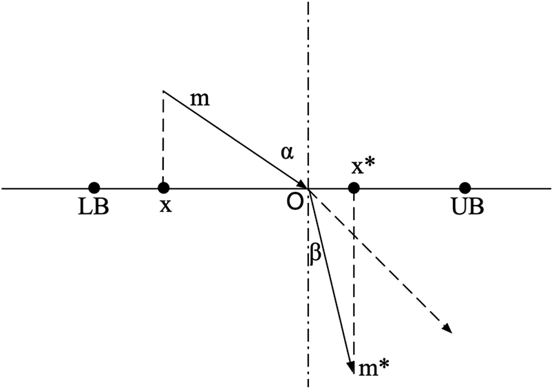
Figure 1: Refracted opposition-based learning

Where the x-axis search interval is known as [LB, UB], the origin O is the midpoint on [LB, UB], α and β are represented by the incidence angle and the refraction angle, respectively. m and m* are the lengths of the incident and the refracted rays, respectively. The above formula can be obtained as follows.

n=sin⁡αcos⁡β=LB+UB2−xx∗−LB+UB2×m∗m(6)

Let σ=mm∗ and n = 1. Substituted into Eq. (6) and expanded to the high-dimensional space of the spider monkey optimization yields the refracted direction solution xi,j∗, as follows.

xi,j∗=LBj+UBj2+LBj+UBj2σ−xi,jσ(7)

where xi,j denotes the position of the spider monkey in the population in j dimensions (i=1,2, ⋯, N;j=1,2, ⋯, D), xi,j∗ denotes the refracted opposition solution of xi,j, LBj, and UBj are the lower and upper bounds of the dynamic boundary, respectively.

3.2 Nonlinear Adaptive Dynamic Weight Factor Strategy

Shi et al. [31] are the first to apply the weight factor ω to particle swarm optimization (PSO). Eq. (2) indicates that the current location is updated according to the local leader’s experience, the spider monkey’s experience within the group, and its own experience. It is easy to lack local search ability in the late iteration. From Eq. (5), it is found that the original location information is ultimately inherited by the new location, and the local search capability of the algorithm is also decreased. Therefore, the introduction of adaptive dynamic weight factor ω is considered in Eqs. (2) and (5).

SMnewij=ω(t)×SMij+U(0,1)×(LLkj−SMij)+U(−1,1)×(SMrj−SMij)(8)

 SMnewij=ω(t)×SMij+U(0,1)×(GLj−SMij)+U(0,1)×(SMrj−LLkj)(9)

ω(t)=ωi+(ωf−ωi)Ps(t)exp⁡(−(αt/Tmax)2)(10)

In Eq. (10), ωi is the initial weight factor, ωf is the final weight factor in the late iteration, α is the non-linear parameter, t is the current number of iterations, Tmax is the maximum number of iterations, Ps(t) is the population success rate, and the calculation steps are as follows.

Taking the minimization problem as an example, the success value S(i,t) is defined as follows:

S(i,t)={1 fit(pbi(t))<fit(pbi(t−1))0 fit(pbi(t))=fit(pbi(t−1))(11)

In Eq. (11), pbi(t) denotes the optimal historical position, fit(⋅) is the fitness function, and the success rate Ps(t) of the whole population based on the success value S(i,t) is formulated as follows.

Ps(t)=1N∑i=1NS(i,t)(12)

In Eq. (12), N is the population size,  Ps(t)∈[0,1].

3.3 Crisscross Strategy

The crisscross strategy [32] is introduced to increase the precision of convergence, but it does not influence the convergence rate.

3.3.1 Horizontal Crossover Operation

The horizontal crossover strategy is to perform crossover operations in the same dimension of different populations. The formula is as follows:

xijt=r1×xijt+(1−r1)×xkjt+c1×(xijt−xkjt)(13)

xkjt=r2×xkjt+(1−r2)×xijt+c2×(xkjt−xijt)(14)

where xijt and xkjt denote the j dimensional generated by the two spider monkeys after later crossover. r1 and r2 are random numbers of [0, 1], and c1 and c2 are random numbers of [−1, 1].

3.3.2 Vertical Crossover Operation

The vertical crossover operation is performed in all dimensions of the newborn individual, and the crossover operation occurs with less probability than the horizontal crossover. The formula is as follows:

xijt=r×xij1t+(1−r)×xij2t(15)

In Eq. (15), xijt is a child individual generated by the j1 and j2 dimensions of individual xijt by longitudinal crossover, r ∈ [0, 1].

3.4 Gauss-Cauchy Mutation Strategy

In the late iteration of the SMO, the rapid assimilation of the spider monkeys is prone to local optimal stagnation. The Gauss-Cauchy mutation strategy [33] is used to mutate the global leader, compare the locations before and after the mutation, and select the better location to substitute into the next iteration, as follows:

Xbestt¯=Xbestt×[1+λ1Cauchy(0,σ2)+λ2Gauss(0,σ2)](16)

Cauchy(0,σ2)=1π(1+x2)(17)

Gauss(0,σ2)=12πe(−x22)(18)

In Eq. (17), Xbestt¯ denotes the location of the optimal individual after mutation, σ2 is the standard deviation of the Gauss-Cauchy mutation, λ1=1−t2/Tmax2 and λ2=t2/Tmax2 are dynamic parameters that adjust adaptively with the number of iterations.

The steps of ISMO are illustrated in Algorithm 1.

The main steps of the proposed ISMO are illustrated in Fig. 2.

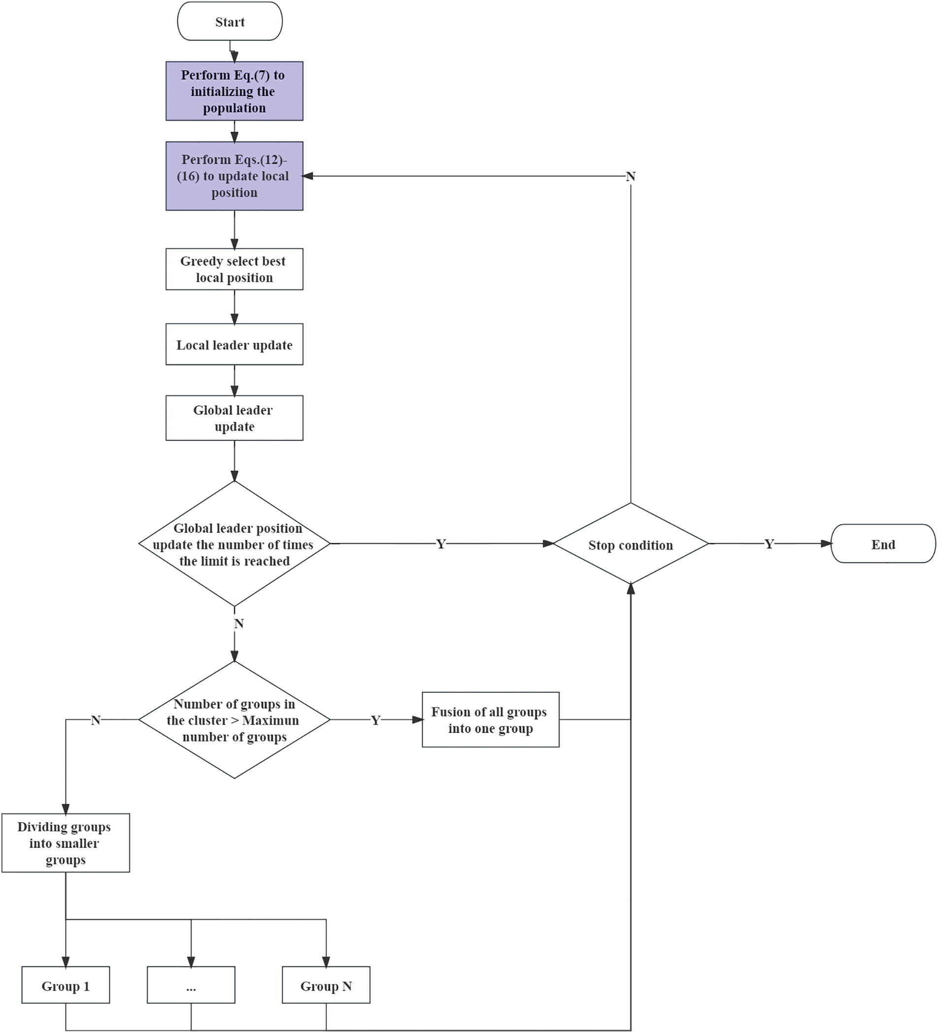
Figure 2: The main structure of the proposed ISMO

4  Experiment Results and Discussion

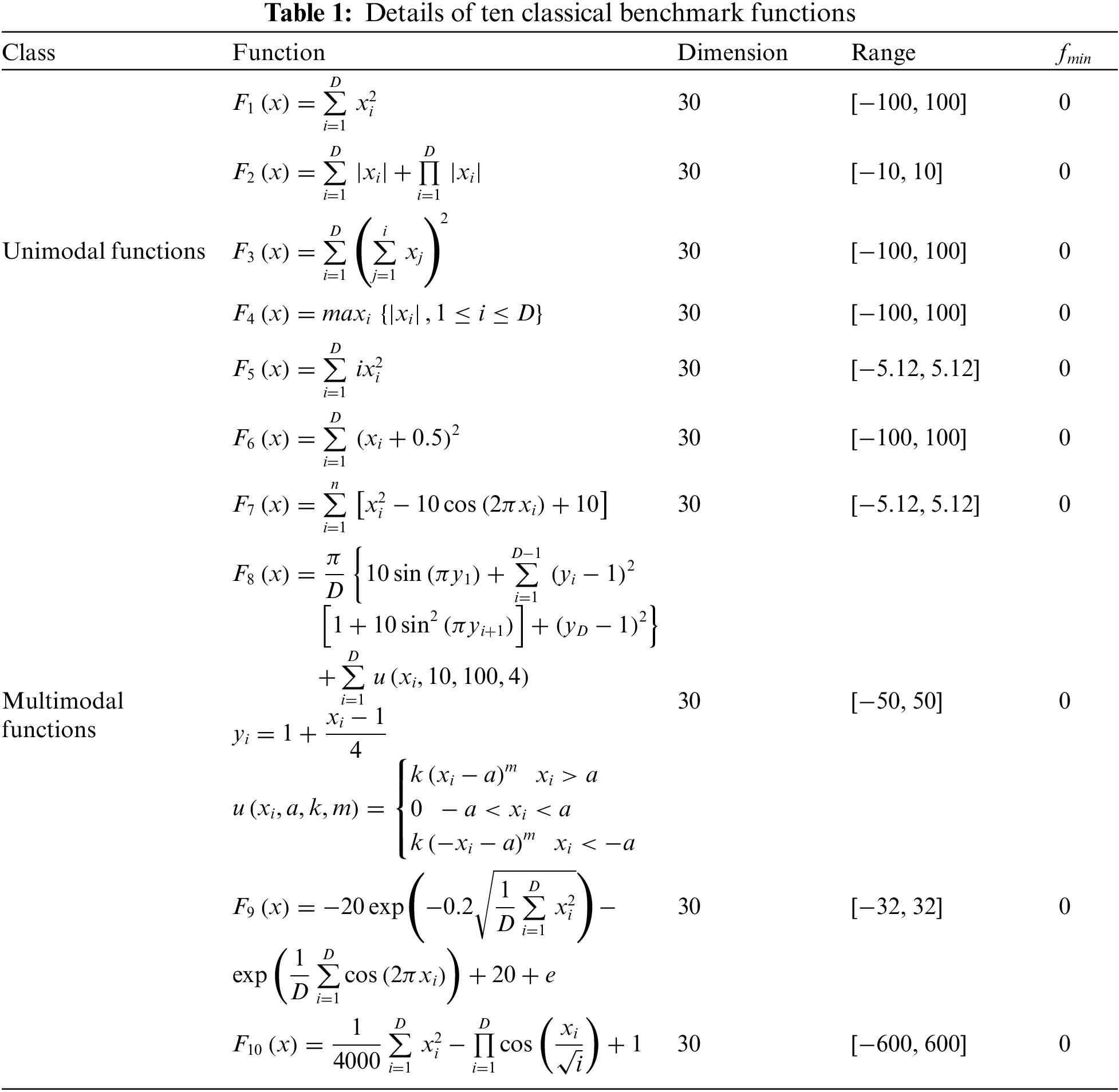
To prove the validity and robustness of ISMO, we choose ten classical unimodal and multimodal functions, in which F1–F6 aims to check the convergence speed and precision, and F7–F10 aims to measure the ability to overcome local optimum, as illustrated in Table 1.

4.1 Comparison Against Other Methods

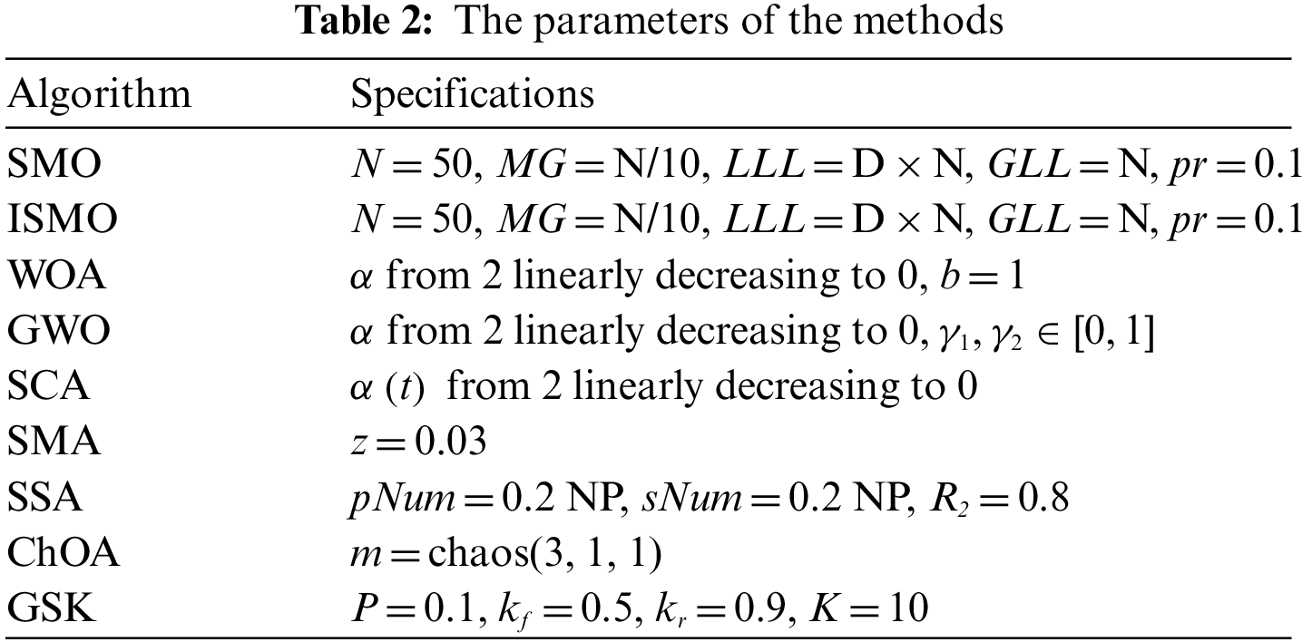
This study selected the performance of the SMO, ISMO, whale optimization algorithm (WOA), grey wolf optimizer (GWO), sine cosine algorithm (SCA), slime mould algorithm (SMA), sparrow search algorithm (SSA), chimp optimization algorithm (ChOA), and gaining-sharing knowledge based algorithm (GSK) for comparison, the parameters of algorithms are described in Table 2.

As shown in Table 3, ISMO is superior to the other eight algorithms for ten benchmark functions. The average (Ave) and the standard deviation (SD) of ISMO are superior to other methods, which indicates that ISMO has better stability and robustness and ISMO can search not only the exploration space but also guarantee global search capability. Detailed results are presented in Table 3, and Fig. 3 illustrates the convergence values of all compared methods on the benchmark functions.

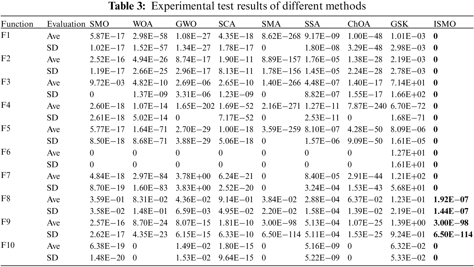
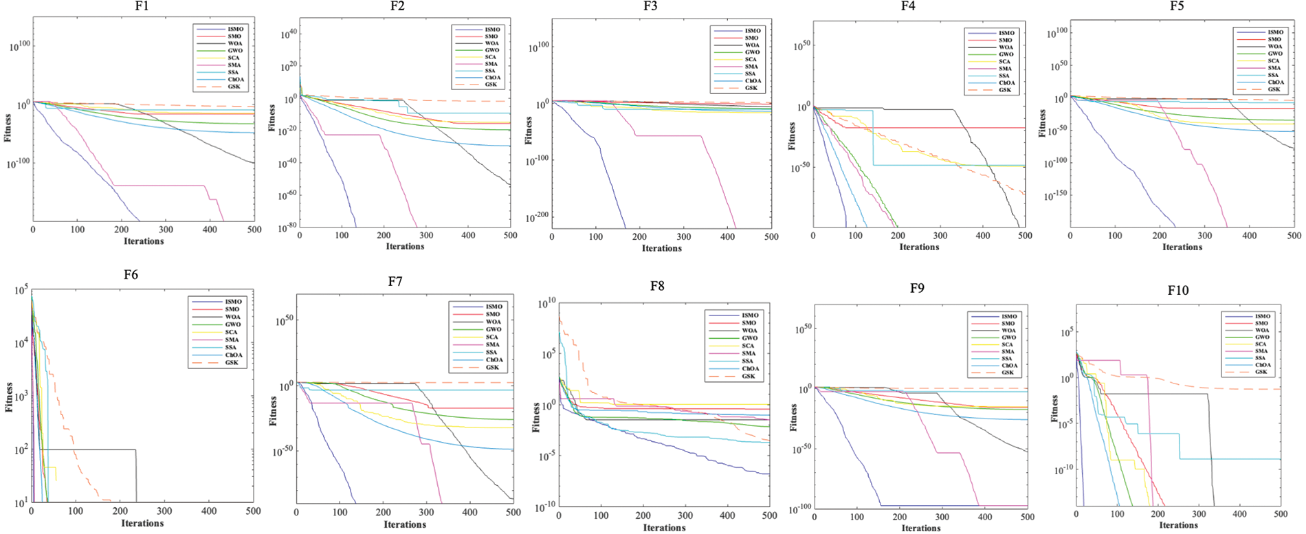
Figure 3: Convergence curves

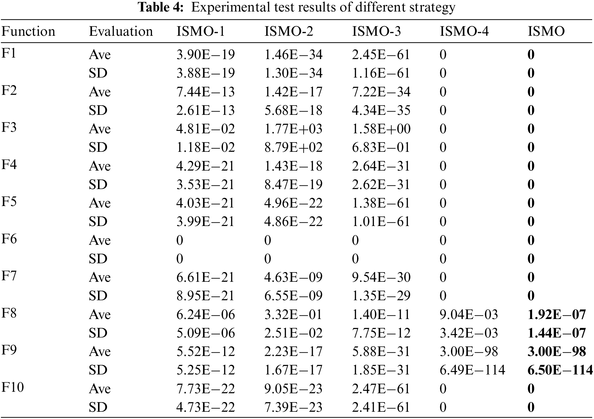
4.2 Impact of Introduced Strategies

In this section, we compare the performance of ISMO with four different search strategies, for example, spider monkey optimization with refracted opposition-based learning strategy (ISMO-1), spider monkey optimization with non-linear adaptive dynamic weight factor (ISMO-2), spider monkey optimization with crisscross strategy (ISMO-3), and spider monkey optimization with Gauss-Cauchy mutation strategy (ISMO-4). From Table 4, the performance of ISMO is superior to other comparison algorithms.

4.3 Nonparametric Statistical Test Analysis

The Wilcoxon signed-rank test and Friedman test [34] are applied to compare the performance of ISMO with other methods, and the significant level is assumed to be 5%. The results of the nonparametric statistical analysis of the ISMO and different methods are presented in Tables 5 and 6, respectively.

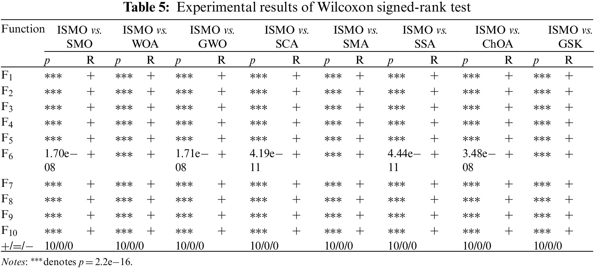
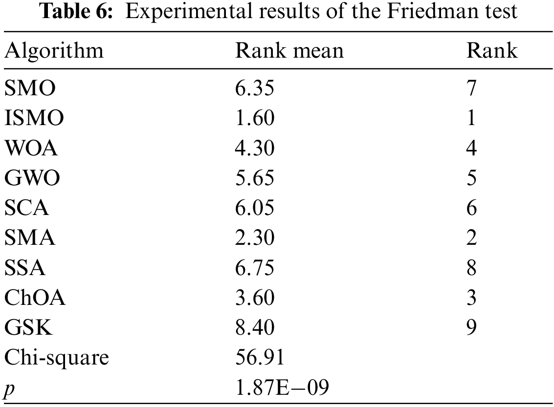
In Table 5, “+,” “−,” and “=” indicate the number of functions where ISMO is superior, inferior, and equivalent to other methods. The p-values of the ten functions are lower than 5%, meaning that ISMO differs significantly from other methods. In Table 6, the average rank of ISMO is 1.60, which is lower than other methods. As a result, the ISMO has been proven to have excellent performance.

5  Feature Selection Optimization Comparison Experiment

5.1 Feature Selection Problem Description

This study applies ISMO to solve the feature selection. Each individual in the overall ISMO represents a combination of features, also called a feature subset. Each dimension is determined by the number of original features in the dataset. Each vector is made up of 0 and 1, where 0 indicates the unselected feature property, and 1 indicates the selection of the corresponding feature property. In the ISMO population initialization, the individual dimension is randomly [0, 1], so the individual vectors in the population consist of 0 and 1. In this study, the values of each dimension above 0.65 are set to 1, and the rest are set to 0 to obtain the individual vectors of 0 and 1.

To balance the minimization of selection features and the maximization of classification accuracy, the fitness function is given by:

F=α×γR(D)+β×|RF||Size|(19)

where γR(D) denotes the classification error rate of a given classifier (the K-nearest neighbor (KNN) classification algorithm is used to evaluate the merit of feature subsets), |RF| denotes the number of features contained in the current individual, |Size| denotes the original number of features in the dataset, α and β denote the importance of the corresponding classification quality and feature subset length, respectively, α and β∈[0, 1], and α + β = 1. In this study, α = 0.99.

To evaluate the performance of ISMO, the mean fitness (Mean), average classification accuracy (ACavg), and average feature selection (FSavg) are chosen as evaluation indicators, and the formula for each indicator is presented in Eqs. (20)–(22).

Mean=1SR∑i=1SRFt(20)

where Ft denotes the run of the optimal solution.

ACavg=1SR∑i=1SRTP+TNP+N(21)

where SR denotes the number of runs, TP, TN, P, and N represent the number of predicted true samples, the number of predicted true negative samples, the number of positive samples, and the number of negative samples, respectively.

FSavg=1SR∑i=1SRRF(22)

where RF denotes the number of optimal feature subsets with element one obtained from each algorithm run.

5.2 Dataset Description

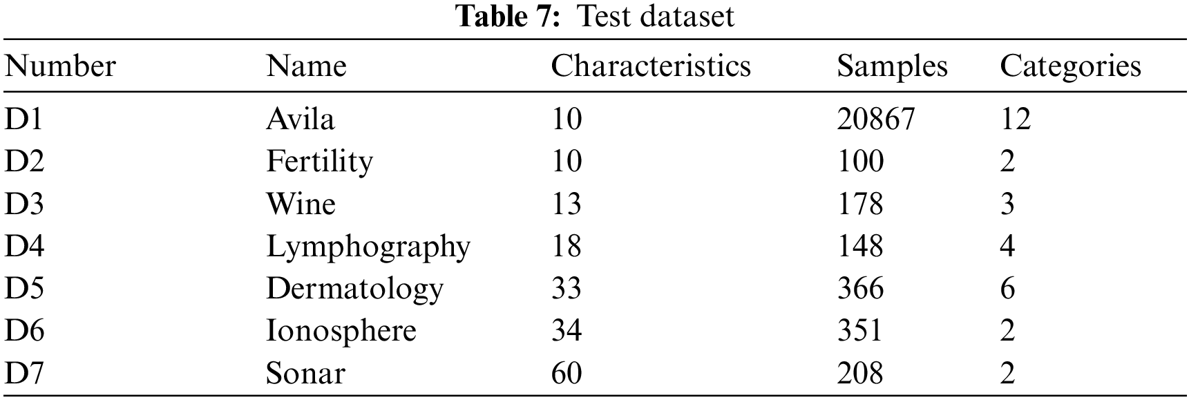
To prove the validity of the ISMO feature selection, we choose seven datasets from the University of California, which are all common test cases for machine learning. A description of the dataset is given in Table 7, including dataset number, name, number of characteristics, number of samples, and number of categories. Ten-fold cross-validation is used for training and testing samples. Every dataset is randomly divided into two groups with different ratios, 90% of the cases are training, and 10% are used for testing. The maximum number of iterations is Tmax = 100, and the result is chosen as the mean of 10 independent experiments. Details of the test dataset are given in Table 7.

5.3 Experimental Results

To compare the overall performance of ISMO, it is compared with other methods, such as grey wolf optimizer (GWO), whale optimization algorithm (WOA), sine cosine algorithm (SCA), and K-nearest neighbor (KNN). Tables 8–10 compare WOA, GWO, SCA, and KNN performance on seven datasets in terms of mean fitness, average classification accuracy, and average feature selections, respectively. The population size is 50, and the maximum number of iterations is 100. Each experiment is run ten times.

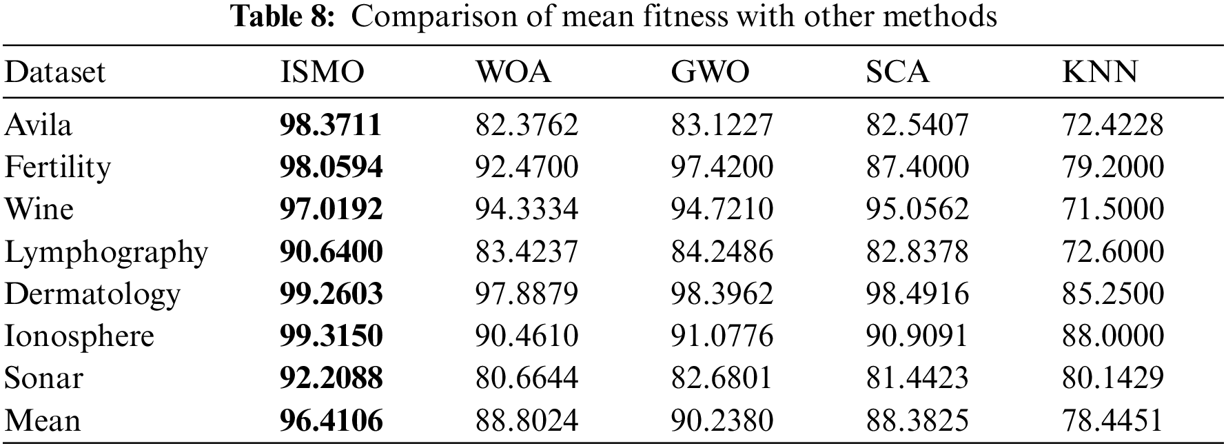
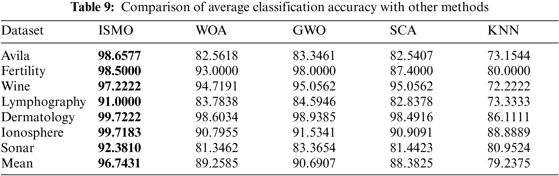
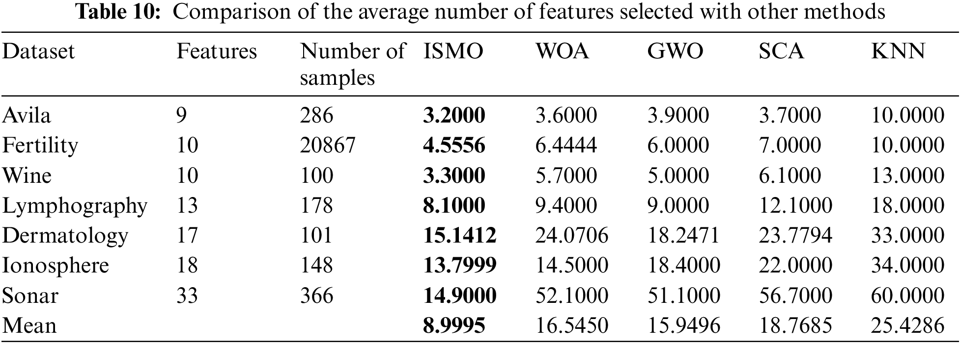
Table 8 shows that the mean fitness of ISMO is superior to WOA, GWO, SCA, and KNN. Notably, ISMO performs significantly better than the KNN, particularly the larger datasets. It is demonstrated that ISMO has excellent performance. Details are given in Table 8 and Fig. 4.

Figure 4: Mean fitness compared with other methods

Table 9 demonstrates that ISMO performs better than WOA, GWO, and SCA on average classification accuracy. The classification accuracy of the classifier trained by the selected feature subset is superior to that of the whole feature set. It is proven that ISMO is effective in reducing the effects of irrelevant and redundant features and improving classification performance. Details are given in Table 9 and Fig. 5.

Figure 5: Average classification accuracy compared with other methods

From Table 10, ISMO achieves the minimum feature count based on the average features. Based on the general average, ISMO finds the least efficient subset of features and performs better than all the other competing algorithms. Therefore, ISMO can be used to select features efficiently, reduce the data dimensionality and simplify the learning model. Details are illustrated in Table 10 and Fig. 6.

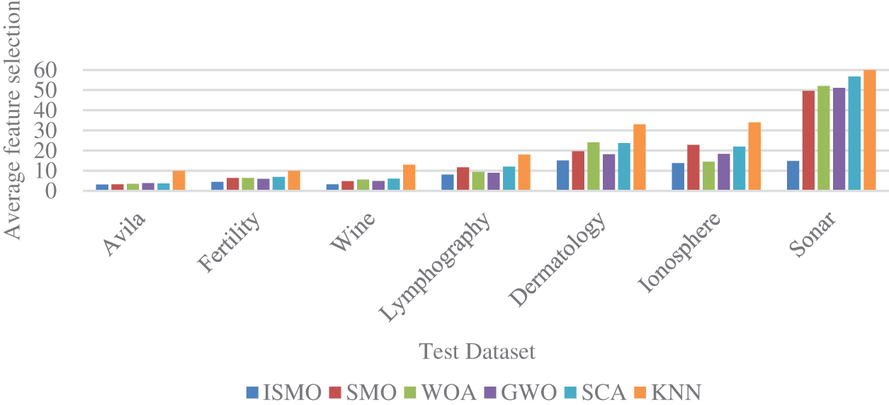
Figure 6: Comparison of average feature selection with other methods

6  Conclusions and Future Research

Aiming at the weakness of SMO, this study presents a new algorithm based on multi-strategy (ISMO). It can draw the following conclusions from the simulation test.

Firstly, inspired by the ideas of refracted opposition-based learning strategy, crisscross strategy, and Gauss-Cauchy strategy, a new position update is proposed to increase the population diversity and enhance global exploration. Moreover, according to the crisscross and Gauss-Cauchy strategies, the target value is updated with mutation to prevent it from getting into the local optimum. Furthermore, to verify the validity of ISMO, we simulated ten benchmark functions and compared them with different methods. Compared with other methods, ISMO has better performance than other methods. Finally, the Wilcoxon signed-rank test and the Friedman test prove that there is a more remarkable difference in ISMO.

Then, the ISMO is validated by the feature selection, and it is proved that ISMO is effective in choosing the best feature subset, reducing the feature dimensionality, and increasing the precision of classification.

Thus, ISMO is likely an excellent solution to numerical optimization problems. In the future, it will be considered how to improve the performance of this algorithm, even in the case of more complicated optimization problems.

Acknowledgement: The authors thank the anonymous reviewers for their valuable comments and suggestions.

Funding Statement: The authors received no specific funding for this study.

Conflicts of Interest: The authors declare they have no conflicts of interest to report regarding the present study.

References

1. J. Gholami, F. Mardukhi and H. M. Zawbaa, “An improved crow search algorithm for solving numerical optimization functions,” Soft Computing, vol. 25, pp. 9441–9454, 2021. [Google Scholar]
2. Y. Rao, D. He and L. Qu, “A probabilistic simplified sine cosine crow search algorithm for global optimization problems,” Engineering with Computers, vol. 38, pp. 1–19, 2022. [Google Scholar]
3. J. L. J. Pereira, G. A. Oliver, M. B. Francisco, S. S. Cunha Jr and G. F. Gomes, “Multi-objective Lichtenberg algorithm: A hybrid physics-based meta-heuristic for solving engineering problems,” Expert Systems with Applications, vol. 187, pp. 115939, 2022. [Google Scholar]
4. I. Fister Jr, X. S. Yang, I. Fister, J. Brest and D. Fister, “A brief review of nature-inspired algorithms for optimization,” arXiv preprint arXiv: 1307.4186, 2013. [Google Scholar]
5. S. Mirjalili and A. Lewis, “The whale optimization algorithm,” Advances in Engineering Software, vol. 95, pp. 51–67, 2016. [Google Scholar]
6. S. Mirjalili, S. M. Mirjalili and A. Lewis, “Grey wolf optimizer,” Advances in Engineering Software, vol. 69, pp. 46–61, 2014. [Google Scholar]
7. S. Li, H. Chen, M. Wang, A. A. Heidari and S. Mirjalili, “Slime mould algorithm: A new method for stochastic optimization,” Future Generation Computer Systems, vol. 111, pp. 300–323, 2020. [Google Scholar]
8. J. Xue and B. Shen, “A novel swarm intelligence optimization approach: Sparrow search algorithm,” Systems Science & Control Engineering, vol. 8, no. 1, pp. 22–34, 2020. [Google Scholar]
9. M. Khishe and M. R. Mosavi, “Chimp optimization algorithm,” Expert Systems with Applications, vol. 149, pp. 113338, 2020. [Google Scholar]
10. J. C. Bansal, H. Sharma, S. S. Jadon and M. Clerc, “Spider monkey optimization algorithm for numerical optimization,” Memetic Computing, vol. 6, no. 1, pp. 31–47, 2014. [Google Scholar]
11. J. H. Holland, “Genetic algorithms,” Scientific American, vol. 267, no. 1, pp. 66–73, 1992. [Google Scholar]
12. R. Storn and K. Price, “Differential evolution a simple and efficient heuristic for global optimization over continuous spaces,” Journal of Global Optimization, vol. 11, no. 4, pp. 341–359, 1997. [Google Scholar]
13. S. Kirkpatrick, C. D. Gelatt and M. P. Vecchi, “Optimization by simulated annealing,” Science, vol. 220, no. 4598, pp. 671–680, 1983. [Google Scholar] [PubMed]
14. R. A. Formato, “Central force optimization: A new metaheuristic with applications in applied electromagnetics,” Prog Electromagnet Res, vol. 77, pp. 425–491, 2007. [Google Scholar]
15. A. W. Mohamed, A. A. Hadi and A. K. Mohamed, “Gaining-sharing knowledge based algorithm for solving optimization problems: A novel nature-inspired algorithm,” International Journal of Machine Learning and Cybernetics, vol. 11, no. 7, pp. 1501–1529, 2020. [Google Scholar]
16. Y. Xu, H. Chen, A. A. Heidari, J. Luo, Q. Zhang et al., “An efficient chaotic mutative moth-flame-inspired optimizer for global optimization tasks,” Expert Systems with Applications, vol. 129, pp. 135–155, 2019. [Google Scholar]
17. P. Agrawal, T. Ganesh and A. W. Mohamed, “Chaotic gaining sharing knowledge-based optimization algorithm: An improved metaheuristic algorithm for feature selection,” Soft Computing, vol. 25, no. 14, pp. 9505–9528, 2021. [Google Scholar]
18. K. Hussain, N. Neggaz, W. Zhu and E. H. Houssein, “An efficient hybrid sine-cosine Harris hawks optimization for low and high-dimensional feature selection,” Expert Systems with Applications, vol. 176, pp. 114778, 2021. [Google Scholar]
19. G. Hu, B. Du, X. Wang and G. Wei, “An enhanced black widow optimization algorithm for feature selection,” Knowledge-Based Systems, vol. 235, pp. 107638, 2022. [Google Scholar]
20. A. Sharma, A. Sharma, B. K. Panigrahi, D. Kiran and R. Kumar, “Ageist spider monkey optimization algorithm,” Swarm and Evolutionary Computation, vol. 28, pp. 58–77, 2016. [Google Scholar]
21. P. Kalpana, S. Nagendra Prabhu, V. Polepally and J. R. DB, “Exponentially-spider monkey optimization based allocation of resource in cloud,” International Journal of Intelligent Systems, vol. 37, no. 3, pp. 2521–2542, 2022. [Google Scholar]
22. R. Menon, A. Kulkarni and D. Singh, “Hybrid multi-objective optimization algorithm using Taylor series model and spider monkey optimization,” International Journal for Numerical Methods in Engineering, vol. 122, no. 10, pp. 2478–2497, 2021. [Google Scholar]
23. K. Gupta, K. Deep and J. C. Bansal, “Improving the local search ability of spider monkey optimization algorithm using quadratic approximation for unconstrained optimization,” Computational Intelligence, vol. 33, no. 2, pp. 210–240, 2017. [Google Scholar]
24. J. Mumtaz, Z. Guan, L. Yue, L. Zhang and C. He, “Hybrid spider monkey optimization algorithm for multi-level planning and scheduling problems of assembly lines,” International Journal of Production Research, vol. 58, no. 20, pp. 6252–6267, 2020. [Google Scholar]
25. H. R. Tizhoosh, “Opposition-based learning: A new scheme for machine intelligence,” in Int. Conf. on Computational Intelligence for Modelling, Control and Automation and Int. Conf. on Intelligent Agents, Web Technologies and Internet Commerce (CIMCA-IAWTIC’06), Vienna, Austria, IEEE, pp. 695–701, 2005. [Google Scholar]
26. T. K. Sharma and M. Pant, “Opposition-based learning ingrained shuffled frog-leaping algorithm,” Journal of Computational Science, vol. 21, pp. 307–315, 2017. [Google Scholar]
27. X. Yu, W. Xu and C. L. Li, “Opposition-based learning grey wolf optimizer for global optimization,” Knowledge-Based Systems, vol. 226, pp. 107139, 2021. [Google Scholar]
28. A. A. Ewees, M. Abd Elaziz and D. Oliva, “A new multi-objective optimization algorithm combined with opposition-based learning,” Expert Systems with Applications, vol. 165, pp. 113844, 2021. [Google Scholar]
29. Z. Wang, H. Ding, Z. Yang, B. Li, Z. Guan et al., “Rank-driven salp swarm algorithm with orthogonal opposition-based learning for global optimization,” Applied Intelligence, vol. 52, no. 7, pp. 7922–7964, 2021. [Google Scholar] [PubMed]
30. F. Zhao, L. Zhang, Y. Zhang, W. Ma, C. Zhang et al., “An improved water wave optimisation algorithm enhanced by CMA-ES and opposition-based learning,” Connection Science, vol. 32, no. 2, pp. 132–161, 2020. [Google Scholar]
31. Y. Shi and R. Eberhart, “A modified particle swarm optimizer,” in 1998 IEEE Int. Conf. on Evolutionary Computation Proc., Anchorage, AK, USA, IEEE, pp. 69–73, 1998. [Google Scholar]
32. A. B. Meng, Y. C. Chen, H. Yin and S. Z. Chen, “Crisscross optimization algorithm and its application,” Knowledge-Based Systems, vol. 67, pp. 218–229, 2014. [Google Scholar]
33. W. C. Wang, L. Xu, K. Chau and D. M. Xu, “Yin-Yang firefly algorithm based on dimensionally Cauchy mutation,” Expert Systems with Applications, vol. 150, pp. 113216, 2020. [Google Scholar]
34. J. Derrac, S. García, D. Molina and F. Herrera, “A practical tutorial on the use of nonparametric statistical tests as a methodology for comparing evolutionary and swarm intelligence algorithms,” Swarm and Evolutionary Computation, vol. 1, no. 1, pp. 3–18, 2011. [Google Scholar]
Cite This Article
Copyright © 2023 The Author(s). Published by Tech Science Press.
This work is licensed under a Creative Commons Attribution 4.0 International License , which permits unrestricted use, distribution, and reproduction in any medium, provided the original work is properly cited.
Downloads
Citation Tools