Adaptive Kernel Firefly Algorithm Based Feature Selection and Q-Learner Machine Learning Models in Cloud

1  Introduction

Cloud CC platforms restrict global complex business models in their services where network play a major role in servicing customers. CC networks are analyzed and researched from all angles [1,2]. CC networks need to be resilient in interactions, security and performances both at administration/user levels [3]. CC’s virtualizations, traffic patterns, networking configurations, and connections are very dynamic and change very often where telemetry signals pass through several transient values in distributions.

PRSs (Pattern Recognition Systems) and MLTs have been used to build predictive models for assessing application performances based on telemetry signals. PRSs train on labelled or unlabelled data to identify unknown patterns. MLTs, based on AI (Artificial Intelligence) are strongly related to recognition of pattern where algorithms aim at providing reasonable outputs for all inputs while considering statistical variations. The success of PRSs and MLTs depend mainly on their suitable selection of features which is also the base for their performances. Thus, FS (Feature Selection) is the core for MLTs success [4,5]. Data features train MLTs while FSs influences their performances with their subset selections from the original feature set and achieve this without transformations and changes to original data. FSs are evaluated based on their ability to discriminate classes based on labelled data and its relevance. FSs work in three types namely filters, wrappers and embedded types. Many studies have found wrappers help in accuracy of FSs which can be also be treated as a combinatorial problem that needs optimization. Bio-inspired algorithms have been used to solve complex combinatorial problems and examples of such optimizations are PSO (Particle Swarm Optimization) and ACO (Ant Colony Optimization). FA (Firefly Algorithm), a bio-inspired algorithm, uses three main procedures namely distance update between fireflies, changing the step size, and solution updates. FA has been found to perform better than traditional PSOs and GAs (Genetic Algorithms) in benchmarks. Further, FAs are popular and generally used on wrapper based FSs. Distributions refer to splitting data and elements between learning models and amongst several nodes for a in large, complex and dynamic variations of data.

This work also uses many algorithms using supervised learning for generating a network security dataset and clustered (unsupervised learning) for segmenting the generated dataset for better classification accuracy. EML (Ensemble Machine Learning) is implemented for benchmarking the proposed DevQMLOps framework. An exhaustive survey on auto-tuning ML models was also conducted in this work and is detailed in the next section.

2  Literature Review

Mabu et al. [6] proposed projections of profits in stock trading systems using EL and rule based MLPs (Multi-Layer Perceptrons). The scheme generated pools of stock trading rules based on a rule-based evolutionary algorithm which were the converted to pools adaptively by MLP selections. These selected rule pools took cooperative decisions on trading of stocks. The scheme’s simulations showed better results in terms of higher profits or losses than methods not using ELs while buying or holding stocks. Sparks et al proposed in their study proposed architecture for automatic scaling of MLTs which included advanced hyper-parameter tuning methods, cost-based cluster resource allocation estimators, and runtime algorithmic introspections for bandwidth allocations, optimal resource allocation and physical resource optimizations. Their TuPAQ (Training-supported Predictive Analytic Query planner) a variation of MLP automatically trained models for user’s predictions. TuPAQ could scale itself to handle Terabytes of data across hundreds of machines more efficiently than standard baseline approaches.

Sparks et al. [7] presented an automatic scaling scheme for MLTs. Their proposal consisted of a NNs (Neural Networks) performance modelling based on an online black-box scheme and a regression based predictor for estimation of metrics after application scaling. Their implementations on varied MLTs showed scaled application’s application-agnostic in terms of reductions in resource costs by 50% when compared with optimal static policy based application scaling, less than 15% reduction of the cost of dynamic policy optimality and equal cost-performance tradeoffs without tuning when compared to threshold-based tuning. Auto scaling for CC applications was proposed by Chen et al. The scheme called SSCAS (Studies on Self-adaptive Cloud Auto-scaling Systems) showed satisfactory results.

Wajahat et al. [8] proposed DevOps practices for MLTs. Their proposal integrated development and operation environments effortlessly. MLT developments and deployments in experimentation phases may be simple, but only careful and proper designs can reduce complexity and execution times. Lack of which can result in significant effects in terms of maintenance or monitoring or improvements. Their proposal applied CI (Continuous Integration) and CD (Continuous Delivery) principles to reduce wastages, support rapid feedbacks, examine hidden technical debts and improve delivery/maintenance/operation functions for applications of MLTs in real-world scenarios.

Chen et al. [9] examined AutoML (Automated MLTs) tools. The study conducted evaluations of these tools with different datasets and data segments. They listed their advantages and disadvantages with test cases. Karamitsos et al. [10] used EL on MLTs for crash analysis. The proposal used k-fold cross-training and averages of RF (Random Forest), ERT (Extremely Randomized Trees), adaptive boosting and gradient tree boosting techniques. The experimental results indicated the superiority of EM based MLT achievements in crash frequency analysis when compared to boosting based EM MLT models in terms of generalization ability/stability and predictive accuracy. They also proposed safety standards in transportation.

Truong et al. [11] studied MLTs on the University of New South Wales UNSW-NB15 dataset for their applicability in detecting new types of intrusions. The MLTs chosen for the study were TS (Tabu Search), TS-RF and RF with wrapper based FS. Their evaluations found TS-RF showed an improved overall intrusion detection accuracy by reduces computational complexity as it eliminated around 60% of the features.

Zhang et al. [12] aimed at NIDS (Network Intrusion Detection System) feature selections. The proposed scheme combined PSO (Particle Swarm Optimization), GWO (Grey Wolf Optimizer), FIFA (FireFly Optimization) and GA (Genetic Algorithm) for improved performances of NIDS. The scheme deployed wrapper-based methods with GA, PSO, GWO and FIFA algorithms for FS using Anaconda Python Open Source and filtered MI (Mutual Information) of the algorithms and generated a set of 13 rules. The derived features were then evaluated using SVM (Support Vector Machine) and J48 classifiers on the UNSW-NB15 dataset. The study’s GA results had better TPRs (True Positive Rates) and FNRs (False Negative Rates). The proposed rule based FS model for NIDS showed improvements in pattern recognitions which could effectively be used for determining novel network attacks as per the Symmetry journal.

Nazir et al. [13] proposed misuse based IDS to find network attacks including DoS (Denial-of-Service), Generic network attacks and Probes. The proposal designed the system based on offline UNSW-NB15 data set for detecting malicious network activities. Their integrated classification model showed better results in comparison to DTs (Decision Trees) based models. The study’s benchmark results of UNSW-NB15 dataset with RTNITP18 set showed higher values on the metrics, false alarm rates, attack detection rates, F-measure, average/attack accuracies in comparison to other existing approaches. Automatic MLT selection for CC was proposed by Almomani [14]. The study tuned the selected MLT models for better builds and better than similar existing methods. The study found that unsupervised learning could explore data spaces quite well until supervised learning models for automations were introduced

3  Proposed Method

This research proposes a dynamic model AKFA for selecting appropriate features ion monitoring CC network operations. This scheme uses DevQLMLOps and Q Learner in its model selections. This work implements different classification (supervised learning) algorithms on the data spaces generated by clustering (unsupervised learning) from the network security dataset in order to segment the data set for better classification accuracy. Most relevant features used for detections are selected via the Adaptive Kernel Firefly Algorithm (AKFA) based FS algorithm. Q learning is mainly used to learn about the quality of FS and advice agents on the features that can used for dynamic classifications. Also, the MLTs introduced for detection have their parameters tuned automatically. The scaling MLTs are analyzed by a Scaling Analyzer and the models are combined using ensemble model AdaBoost. The final outputs are then evaluated using performance metrics. Fig. 1 depicts the overall flow of the proposed research work.

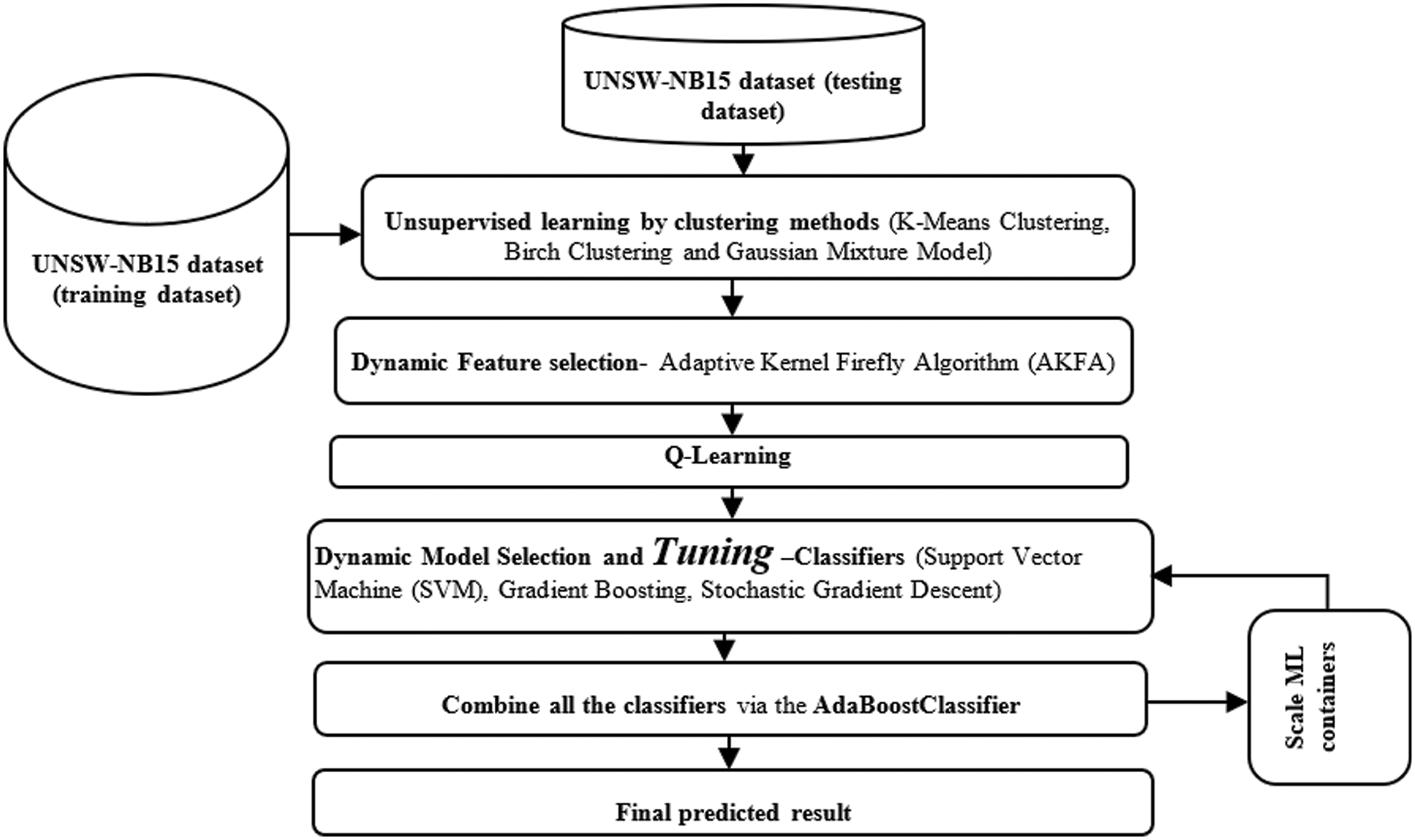
Figure 1: Overall flow of the proposed research work

3.1 UNSW-NB15 Dataset

This study chose the UNSW-NB15 dataset [15–20] to train proposed MLTs as the dataset contains network anomaly and IDS data collected from online data generated using known traffic generators like IXIA, Bro-IDS and Argus [21–26]. Three categorical variables namely proto, state and service are in text form. The fist describes the protocols used in packet transmissions like TCP, UDP etc. Service refers to the network service used by the protocols like SSH, SSL etc. The state parameter refers to the status/type of request like interrupts, connection etc. Network pakets captured in the dataset indicate features of normal transmissions and attack details. The dataset has 82,332 training samples and 1,75,341 testing samples. The data types used are text, binary, nominal, float and integer. Information on port numbers, IP (Internet Protocols) addresses also exist with labels on attacks and normal packets. Most MLTs process text based categorical values by converting them into numeric values using label encoding techniques and also normalizes large values measured with different scales to common scales.

3.2 Label Categorization for Supervised Learning

The dataset’s attack name feature with 10 categorical text defines 9 different attacks and NO-ATTACK description. This label can be used by supervised MLTs for multi-class classification by converting them into multiplicity of binary classifiers which assign 1 or 0 to the data samples based on presence or absence of an attack type. The classifiers are iterated 10 times once for each categorical and their accuracies are stored.

3.3 Unsupervised Learning for Clusters

Labels like Fuzzers or Exploits generate lower prediction accuracies which are improved using unsupervised algorithms as they easily find inherent groups/clusters in such samples. They are also highly similar in their intra-cluster values with low inter-cluster values. MLTs first partition the UNSW-NB15 training dataset to form clusters which are then processed using clustering techniques K-Means, Birch and Gaussian mixture models. The accuracies of label predictions for the different clusters are measured.

3.4 DFS (Dynamic Feature Selection)

DFS is an automatic selection of features from the dataset for predictions. DFSs select minimal and probable features that represent a miniature set of actual features. DFSs have other advantages like reducing dimensionality, over fitting and training times. Adaptive Kernel Firefly Algorithm (AKFA’s) DFS is a novel technique based on evolutionary computation and inspired by firefly’s behaviour. Different MLTs find feature importance which change in time slots i.e. Feature set Fs = {f1,f2, f3} to time slot ts1 but not be the same for time slot ts2 in label predictions. Thus, a new model that uses most important features is needed where DFS and tuning are used. FA used in this work is based on three things as detailed below where Fireflies are features and brightness implies accuracy:

(i) Fireflies get attracted to others in the species based on brightness (Fitness Function).

(ii) Fireflies having higher brightness values attract other fireflies.

(iii) Fireflies with lesser brightness values move towards brighter ones.

These basic behaviors fireflies inspired in building the FA optimization algorithm where their behaviours is connected to the construction of FA. Each dynamic feature analogous to an optimal solution is based on its brightness value or classification accuracy. Features with lower accuracy values tend to move towards higher accuracies mimicking brightness. FA iterates this new solution of feature based on brightness comparison between old and new. Only newly selected feature solution sets are retained replacing older ones. Assuming each solution firefly i (Fi) is a feature position of an iteration, the classification accuracy of i is higher than another solution j and the distance between them can be computed using Eq. (1).

rij=(Fi−Fj)2 (1)

The distance computations are followed by updates substituted in Eq. (2) to computer new attractiveness and the new feature position for ith firefly can be found corresponding to newly selected ith solution and the procedure is carried out based on Eq. (3).

β=β0e−γrij2 (2)

Fijnew=Fi+β.rand.ΔFij+rand (3)

where, rand–random number of i, β0 –attractiveness at 0 distance and is generally set to 1, Fj –fitness function < Fi and .ΔFij –updated step size using Eq. (4),

ΔFij=(Fj−Fi) (4)

Eqs. (1)–(3) determine the ith solution iteratively until no solution lesser than lower fitness function exists. Thus, each selected feature solution i may have a higher solution or no solution based on fitness comparison between i and other solutions in the current dataset (population) and can be equated to Eq. (5)

Finew={Fi, if Fiis FGbestFiGbestnew, if Fiis FGbestFijnew with FTbest else (5)

If selected feature solution i Eq. (5) is the global best feature solution, further feature solutions are not generated. In case it is second, only one new feature solution, FiGbestnew is generated for Fi and FGbest is the global best solution amongst samples. For third best or worse than the third best solution s for Fi , two new solutions to Npop − 1 and Fijnew are generated. Thus, the set of new solutions of i is evaluated to compare the best with the lowest and best is retained while others are discarded. FAs have many disadvantages like premature convergence to local optimum or convergence to near global optimum with high iterations. To overcome these difficulties this work uses three parameters namely attractiveness β (kernel), updated step size ΔFij , and random number (rand) in Eq. (3). These improvements are detailed below

Improvement Stage 1: This work uses FGbest for computing values based on RBF (Radial Basis Function) kernel depicted in Eq. (6) instead of considering distances i and better feature solution to determine the kernel. RBF kernel’s features Fi and FGbest are feature vectors in the input space

Kibest=exp⁡(−||Fi−FGbest||22σ2) (6)

FGbest Replaces Fj in Eq. (1) as it is more effective in scaling β which is a function of radius Eq. (1). This improvement showed as better AKFA results in comparison to FA results in terms of optimal solutions found by AKFA’s search ability and reflected via SD (Standard Deviation) values.

Improvement Stage 2: AKFA in the second stage generates an updated step size. The updated step size of Eq. (4) is similar to DEA (Differential Evolution Algorithm) mutations where β is the mutation factor between 0 and 2. The proposed improvements are depicted in Eqs. (7) and (8).

ΔF1ij=FGbest−FWorst (7)

ΔF2ij=(Fj−Fi+Fr1−Fr2) (8)

where, r1, r2 denote random numbers. It is evident that ΔF1ij (1st updated step size) < ΔF2ij (2nd updated step size). The use of ΔF1ij or ΔF2ij is based on fitness ratio values given in Eq. (9)

ΔFij={ΔF1ij,  ifFRi>FRNpopΔF2ij, else (9)

where, FRi , FRNpop are not control parameters and assume variable values given by Eqs. (10) and (11)

FRi=FTi−FTGbestFTGbest   (10)

FRNpop=FTNpop−FTGbestFTGbest (11)

It is evident that two possibilities for comparison between FRi and FRNpop exist and FRi can be lesser or higher than FRNpop . Updated step size ΔF2ij should be > ΔF1ij to eliminate obtained new selected feature selection solution from current good feature solutions and thus avoid falling into the local optimum zone and effectively avoid premature convergence. When feature solution of i is lesser than the average solution, it is not near to good solutions and searches around using a larger step size.

Improvement Stage 3: The proposed work in the third stage of improvement uses normal distributions (randn) in place of uniform distributions (rand) based on Eq. (12):

FijNew=Fi+β.Randn.ΔFij+Randn (12)

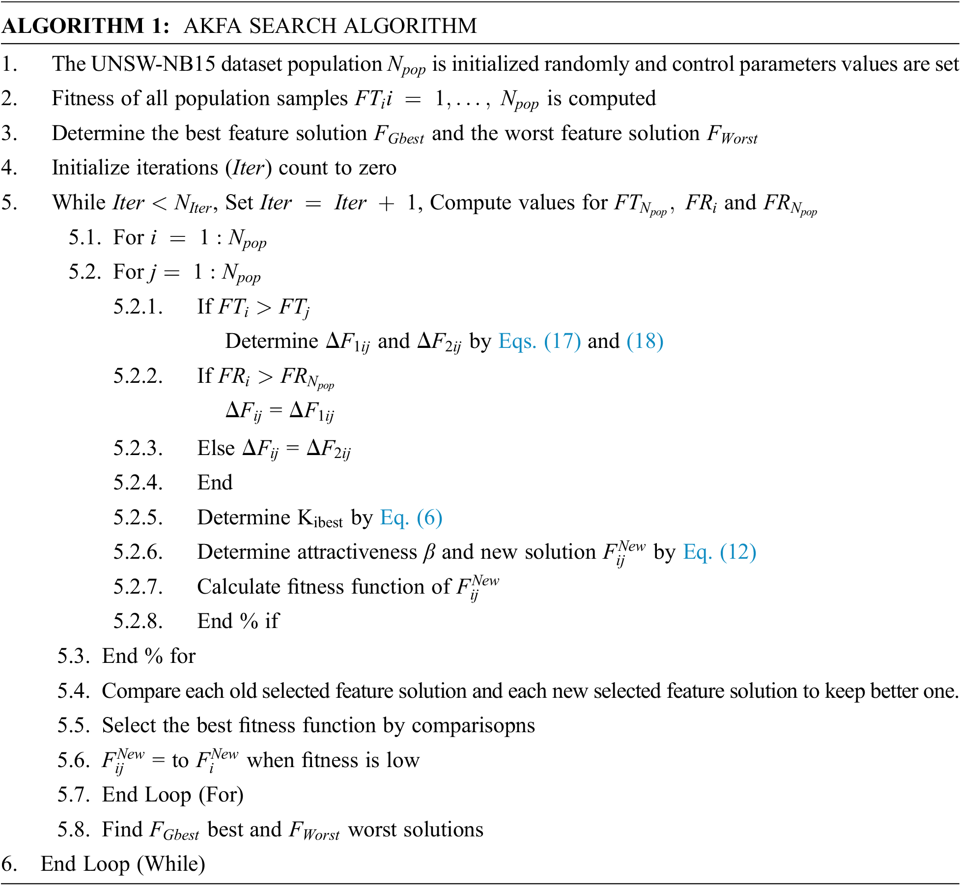
The AKFA DFS architecture is depicted in Fig. 2 which is followed by the description of AKFA search in Algorithm 1.

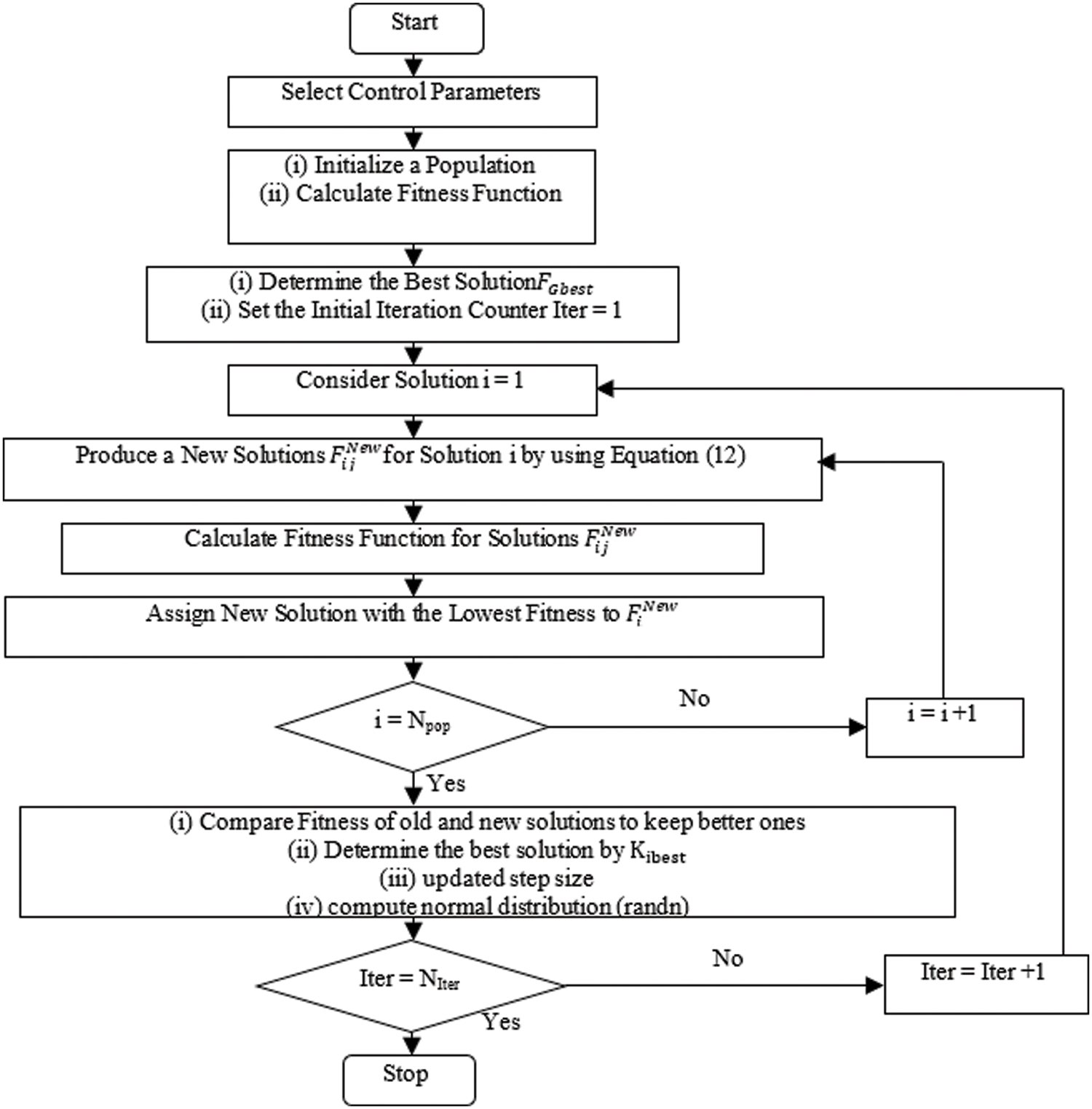
Figure 2: AKFA DFS architecture

3.5 Q-Learning

Q-learning is a RL (Reinforcement Learning) that is non-dependent on models and learns quality of classifications by instructing agents to consider classifiers based on criteria. The operation includes an agent, a set of states S (Selected Features) and set A(classifiers) per state. In a classification  (a∈A) the agent transits from one state to another. This execution of classificationin a specific state generates classification accuracy (reward). On performing this sequence of actions, the agent finally obtains a total reward called the Q-value given as Eq. (13)

Q(s,a)=r(s,a)+γmaxa⁡Q(s′,a)  (13)

From Eq. (13), Q-value obtained from state s on performing action a is the reward r(s,a) in addition to highest obtainable Q-value from the next state s′.γ controls the contribution of future classification accuracy and Q(s′,a) is dependent on Q(s′′,a) where a coefficient of γ 2. Hence, Q-value depends on Q-values of future states as shown in Eq. (14).

Q(s,a)=γQ(s′,a)+γ2Q(s′′,a)….,γnQ(s′′….n,a) (14)

Changing the value of γ gamma change the contribution levels of classification accuracy. Being a recursive Eq., it starts with arbitrary assumptions for q-values and over a period of time/experience, it converges to optimality. In applications it is an update given by Eq. (15)

Q(St,At)←Q(St,At)+α[Rt+1+γmaxa⁡Q(St+1,a)−Q(St,At)]                   (15)

where α –step size (learning rate) or determines the extent of overwriting of old information by new information.

3.6 Dynamic Model Selection and Tuning

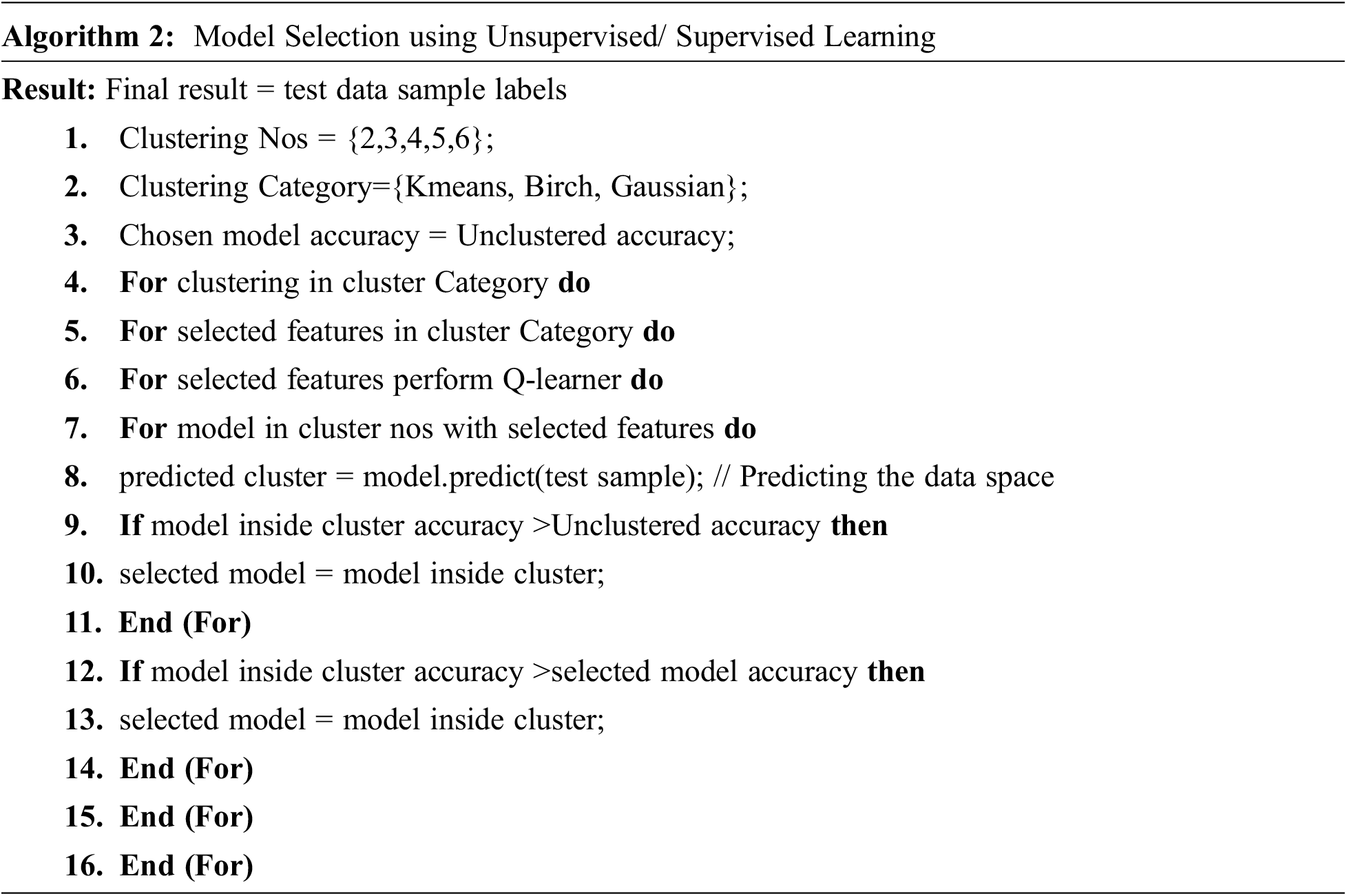
There is a need for automatically selecting accurate models based on the real time data. As explained in the previous section, multiclass classification can be converted into a multiple binary classifications for improving cross validation accuracy. Using weighted majority rule based on voting is one technique for the aforesaid automatic selections. Voting weights are determined by generated prediction accuracies of models. If escalating cluster counts does not enhance classifier accuracies in clusters, then accurate classifiers are identified by using their cross-validation accuracy score across clusters. This model selection is listed as Algorithm 2 [23]. The model auto-selection DevQLMLOps using weighted majority voting is depicted as Fig. 3.

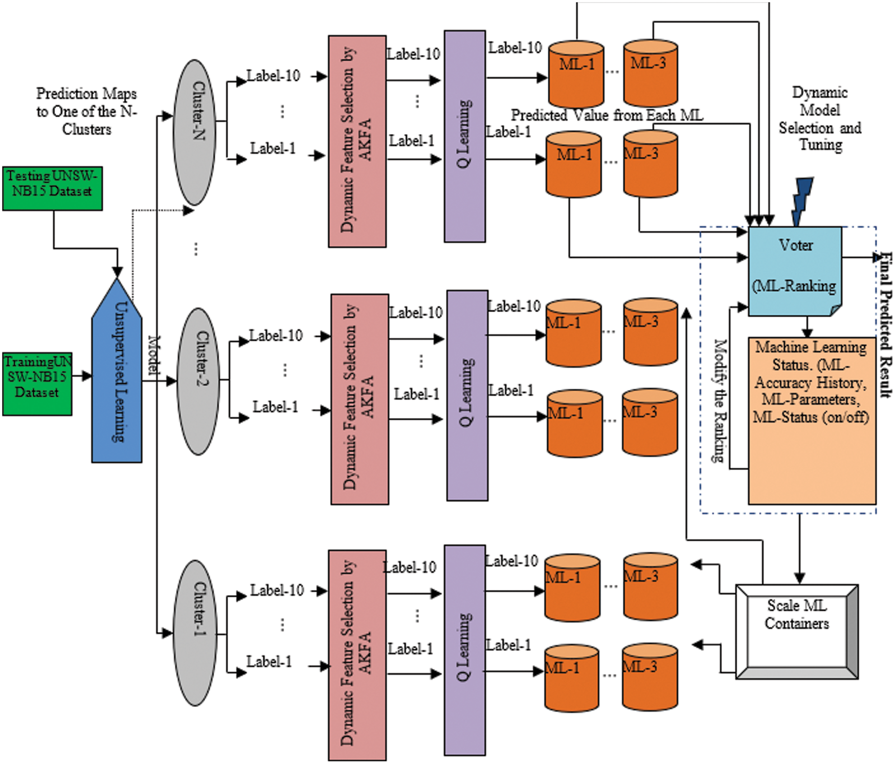
Figure 3: Reflexive devqlmlops architecture for autoselection and autotuning

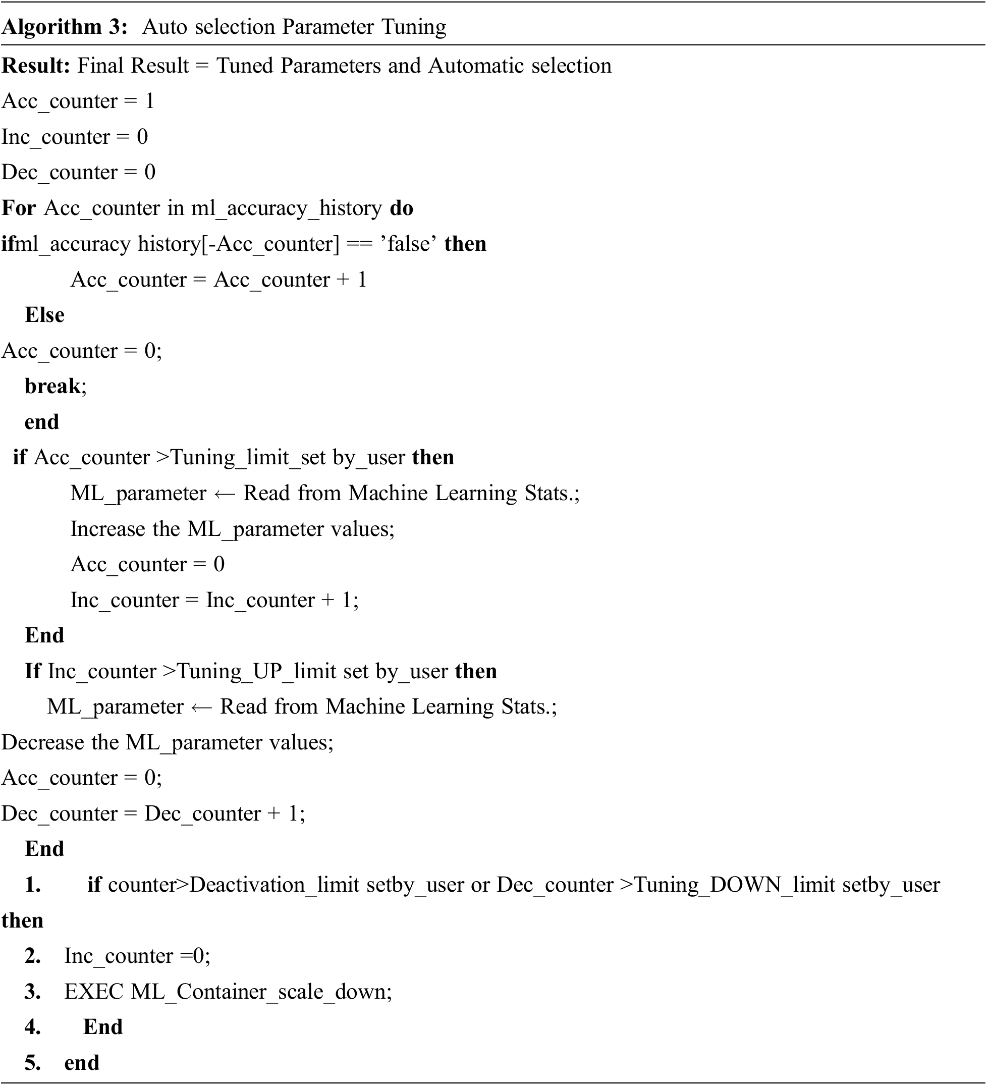
DevQLMLOps is used in this work as its parameters get adapted while tracing accuracy in models and records significant accuracy improvements. This work’s adaptive methodology is a necessary parameter tuning step before a model is discarded in automatic selections of models. This tuning of parameter is depicted in Fig. 3 and listed as Algorithm 3.

“ML Stats” which stores each ML model’s parameters and a sub-module of “Dynamic Model Selection and Tuning”. Models crossing threshold value of consecutive erroneous predictions have their parameters tuned accordingly based on the direction of threshold crossing (UP/DOWN). The tuned parameters are passed again to the model’s docker containers through Scaling Analyzer module. On reaching all limits which are set by the user based on dataset’s pattern or a data space time window, the docker is deactivated. As an example, an online dynamically changing data stream based on time frames was simulated for data spaces creation. Test data was split into 17 time windows with ten thousand records in each time window. The selected auto-tuning parameters were estimators (n), individual regression estimator’s maximum depth (max depth) for limiting tree node counts, minimum count of samples in splitting an internal node (min samples split), and feature count to be considered for best split (max features) The default values used in initial experiments of data spaces were n = 100, max features = none, max depth = 3 and min samples split = 2. Further experimentations parameters were tuned UP based on Algorithm 3 for every data space time window’s beginning and differences between the two experimental accuracy values was observed in most of the data spaces.

3.7 EML

EMLs have been used quite extensively with the aim of combining predictions of multiple estimator’s learning model for improved robustness and accurate outputs. AdaBoost and XgBoost are famous EML models. This research work uses AdaBoost.

3.7.1 SVMs (Support Vector Machines)

SVMs operate on a single principle that of creating the best demarcation boundary (hyperplane) for n dimensional data into two predictable classes i.e. attacker or normal. SVMs select extreme vectors (support vectors) in their process of hyperplane creations. SVM’s classification is depicted as Fig. 4 where the decision boundary is demonstrated. The advantage of SVM is that it works relatively well when there is a clear margin of separation between classes. SVM is more effective in high dimensional spaces.

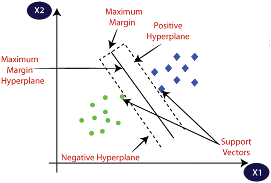
Figure 4: SVM hyperplane classification

SVMs creation of the hyperplane can be depicted as Eq. (16)

w.x+ b= 0, xi∈Rn (16)

Separation of data points xi in the UNSW-NB15 dataset amount to isolating xi as a class on the same side of the plane based on a decision rule [17] given as Eq. (17):

g(x)= sign(w.x+b) (17)

Assuming l patterns exist where each pattern has a pair {xi, yi}i=1N and vector xi∈Rn(patterns) has a label yi∈{−1, 1} . If X⊂Rn and Y (labels)⊂{−1, 1} . SVMs aims to classify using Eq. (18)

y(x)= sign[∑i=1N⁡αiyiK(xi,x)+b] (18)

where αi , b–real constants, K(xi,x)=⟨ϕ(xi),ϕ(x)⟩,⟨.,.⟩ –inner product operation, ϕ(x) –nonlinear mapping from original data space to a high dimensional space. Assuming the data can be demarcated using a linear hyperplane in the high dimensional space, it can be depicted as Eq. (19),

yi[wTϕ(xi)+b]≥1, i=1,….N (19)

And when a hyperplane is not found/exists, a slack variable n is used as in Eq. (20)

yi[wTϕ(xi)+b]≥1−ξi, i=1,….N, ξi≥0, i=1,….N   (20)

Thus attacks are detected from the UNSW-NB15 dataset.

3.7.2 GBA (Gradient Boosting Algorithm)

GB is a MLT that can classify the dataset UNSW-NB15 and can join weak learners into a strong learner iteratively. The least-squares regression setting for teaching a model F to predict values can be equated to Eq. (21)

y^=F(x) (21)

And mean squared error reductions are done using Eq. (22)

MSE=1n∑i=1n⁡(y^i−yi)2 (22)

where, I–training set indices, y–output variable (attack detection), y^i –predicted value of F(x), yi –observed value from x, n–samples count in y.

If GBA has M stages, then at each stage of GB, an imperfect model Fm for low m returns y^i=y¯ }, where the RHS (Right Hand Side) is the mean of y. Estimator hm(x) is added to improve the model as depicted in Eq. (23),

Fm+1(x)=Fm(x)+hm(x)=y (23)

GBA will fit h to residual y − Fm(x) . Boosting variants ( Fm+1 ) correct predecessor’s errors. Generalization of function losses other than squared error in classification/ranking problems, it can be observed that residuals hm(x) of s model are negative gradients of loss MSE (Mean Squared Error) w.r.t F(x) as in Eqs. (24) and (25)

LMSE=12(y−F(x))2 (24)

hm(x)=−∂LMSE∂F=y−F(x) (25)

GB could be specific to a gradient descent, generalizing its entails to loss and gradient. The advantage of GBA is Often provides predictive accuracy that cannot be trumped. Lots of flexibility which can optimize on different loss functions and provides several hyper parameter tuning options that make the function fit very flexible.

3.7.3 Stochastic Gradient Descent

SGD (Stochastic Gradient Descent) is an iterative optimizing objective function with appropriate smoothness properties like differentiable or sub-differentiable properties. It is a stochastic approximation of gradient descent optimizations as replaces actual gradients computed from the whole data setby estimating randomly selected subsets. GDA trains all samples in training set for one update of one parameter in an iteration. SGDs use only one training sample from the training to update a parameter in an iteration. The algorithm is used in logistic regression to update the weights. SGD being an online learning algorithm, can incrementally update classifier as new data arrives instead of updating all at once. GDA’s update parameter θ of the objective F(θ) is given as Eq. (26),

θ=θ−α∇θE[F(θ)] (26)

where, E[F(θ)] − GDA evaluation cost over the complete training set. SGD uses only one or limited training examples and its update is given by Eq. (27),

Θ=θ−∇αF(a(i),b(i)) (27)

In the pair (a(i), b(i)) from the training set. Ultimately, majority voting over the current voting set ensues for combining results of the aforesaid classifiers. The advantage of SGD is for larger datasets it can converge faster as it causes updates to the parameters more frequently.

3.8 ML Container Scaling

Scaling Analyzer module tunes ML model parameters stored in ML Stats sub-module and follows rules for scaling which are listed below:

(A) Prediction Error Rule: A model making erroneous predictions for S (User Defined) consecutive samples is given the state ”OFF” as it results in inaccuracies affecting weighted majority voting.

(B) Time-out Rule: Every model is executed within a docker container and might get timed out due to congestion in the network or on completion of its allotted time limit. A model scoring R (User Defined) consecutive timeouts is set to the ”OFF” state, the container is discarded and another container with similar parameter values is activated.

(C) Tie-breaking Rule: If M is count of models and voting results of two labels for P (User Defined) consecutive samples are closer to a tie and count of active models <M, an OFF model is turned on for getting out of the tie-breaking situation.

(D) Inaction Rule: If active ML model count <M for Q (User Defined) consecutive samples, OFF models are activated for including their predictions in the weighted majority vote and models go OFF based on Time-out Rule or Prediction Error Rule.

4  Results and Discussions

The measured results of classifiers are displayed in this section. UNSW-NB15 dataset was used in training/ testing MLT implementations. These algorithms explained in Section 3.1 were applied on the dataset and measured for precision, recall, F-measure and accuracy. Precision is the fraction of accurately classified attacks against all attack records. Recall is a fraction of perfectly classified attacks against the number of accurately classified attacks and misclassified attacks. Precision is depicted in Eq. (28),

Precision=TPTP+FP (28)

Recall=TPTP+FN (29)

Recall evaluates in terms of TP (True Positive) in relation to FN (False Negative) entities and mathematically as Eq. (29):

F1-Measure is the computed average of recall and precision and computed using Eq. (30):

F1−Measure=2∗Precision∗RecallPrecision+Recall (30)

Accuracy=TP+TNTP+FP+FN+TN (31)

Accuracy is correctly classified instances as normal/attack classes and the percentage of correctly classified records over the count of data set rows irrespective of correctly or incorrectly classified, as reflected in the following Eq. (31)

In this section the above mentioned metrics have been measured using the classifiers like AdaBoostClassifier, XgBoost, Dynamic Auto selection and Auto tuning (DASAT), and proposed DASAT with Q Learner (DASATQL) (See Table 1).

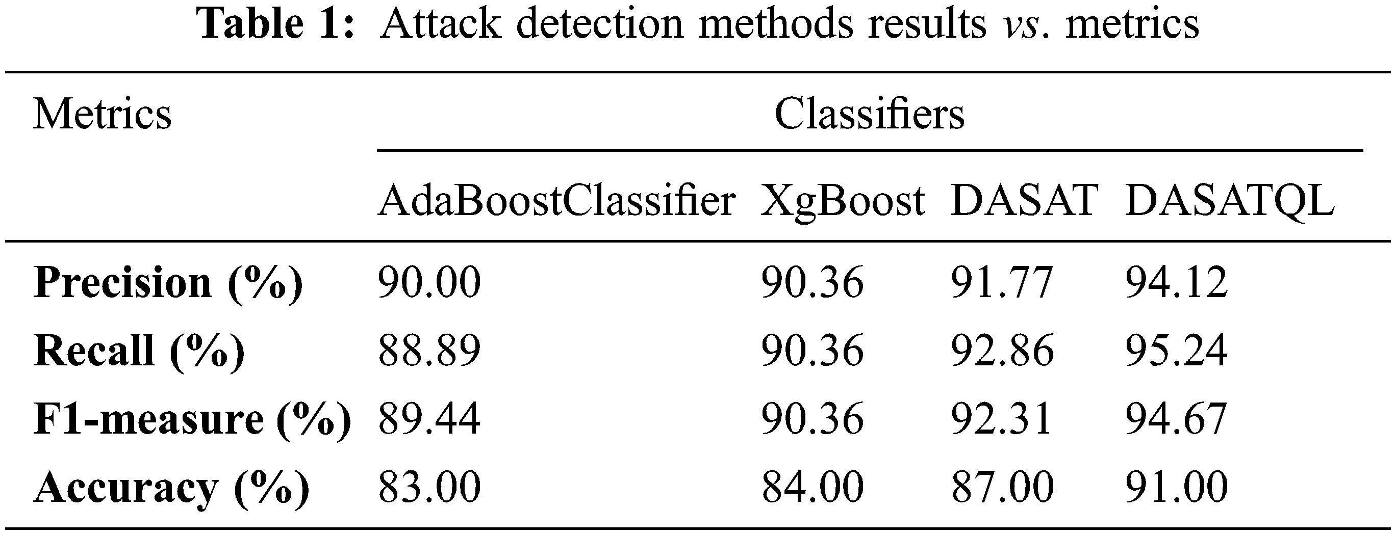
Fig. 5 shows the performance comparison results of proposed DASATQL classifier and existing classifiers such as AdaBoostClassifier, XgBoost, and DASAT via the metrics like precision, and recall. DASATQL classifier has shown the best results for both metrics when compared to existing traditional machine learning models. The proposed DASATQ classifier gives higher precision results of 94.12%, whereas other methods such as AdaBoostClassifier, XgBoost, and DASAT achieves precision of 90.00%, 90.36%,& 91.77% (See Table 1). It is found that proposed DASATQL classifier show great results in attack detection since the proposed work Q learner is introduced to existing methods which may increases the results of the attack detection than the normal classifier. Finally, DASATQL classifier exhibits high performance on metrics. The results comparison of proposed DASATQL classifier and existing classifiers such as AdaBoostClassifier, XgBoost, and DASAT with respect to F1-measure and accuracy results are shown in the Fig. 6. The proposed DASATQL classifier gives higher accuracy results of 91.00%, whereas other methods such as AdaBoostClassifier, XgBoost, and DASAT achieves accuracy of 83.00%, 84.00%,& 87.00% (See Table 1). It is found that proposed DASATQL classifier show great results in attack detection since the proposed work optimal features are selected via AKFA and Q –learner is introduced between the feature selection and classifier. The Q leaner will automatically update the selected features to the training set, so there is no need for the creation of the dynamic classifier each and every time. Once the features are selected it is automatically updated for present features which may overcome the gap between the feature selection and classifiers with increased accuracy. Finally, DASATQL classifier exhibits high performance on metrics.

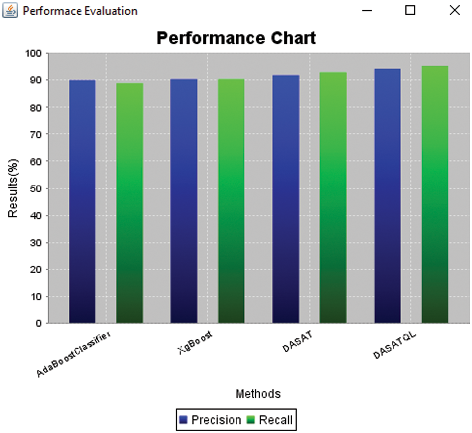
Figure 5: Precision and recall results comparison of attack detection methods

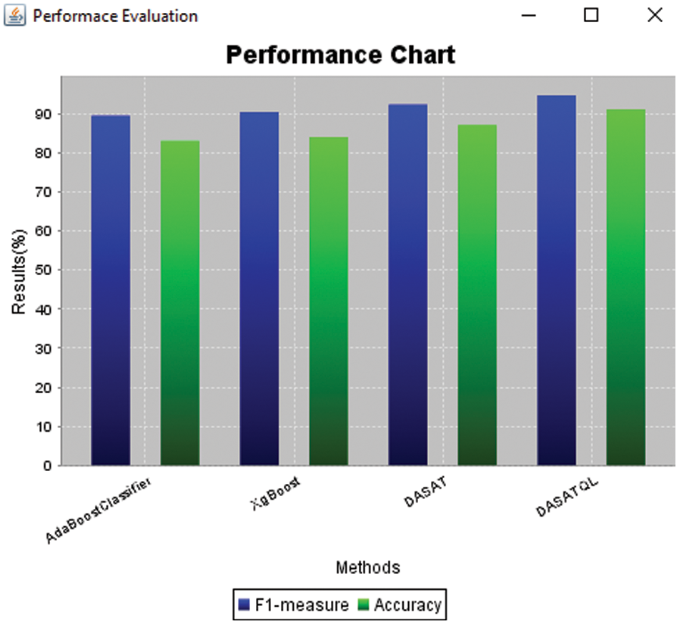
Figure 6: F1-measure and accuracy results comparison of attack detection methods

From Fig. 7 it is evident that the proposed DASATQL classifier has higher cross validation with 94.835% than other classifiers cross validation scores of 86.81%, 89.78%, and 92.545% for 10 dataset labels. Cross-validation accuracies of label predictions are depicted in Fig. 8. The Reflexive DevMLOps setup’s accuracy is better with 85% for all the label predictions (Refer Table 2).

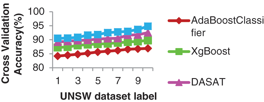
Figure 7: Statically-tuned el accuracy

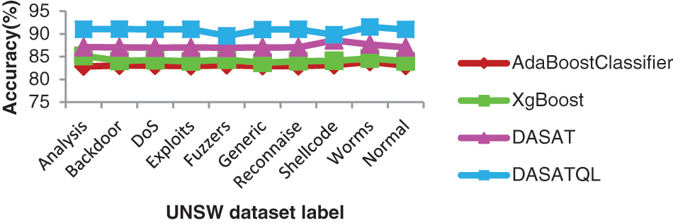
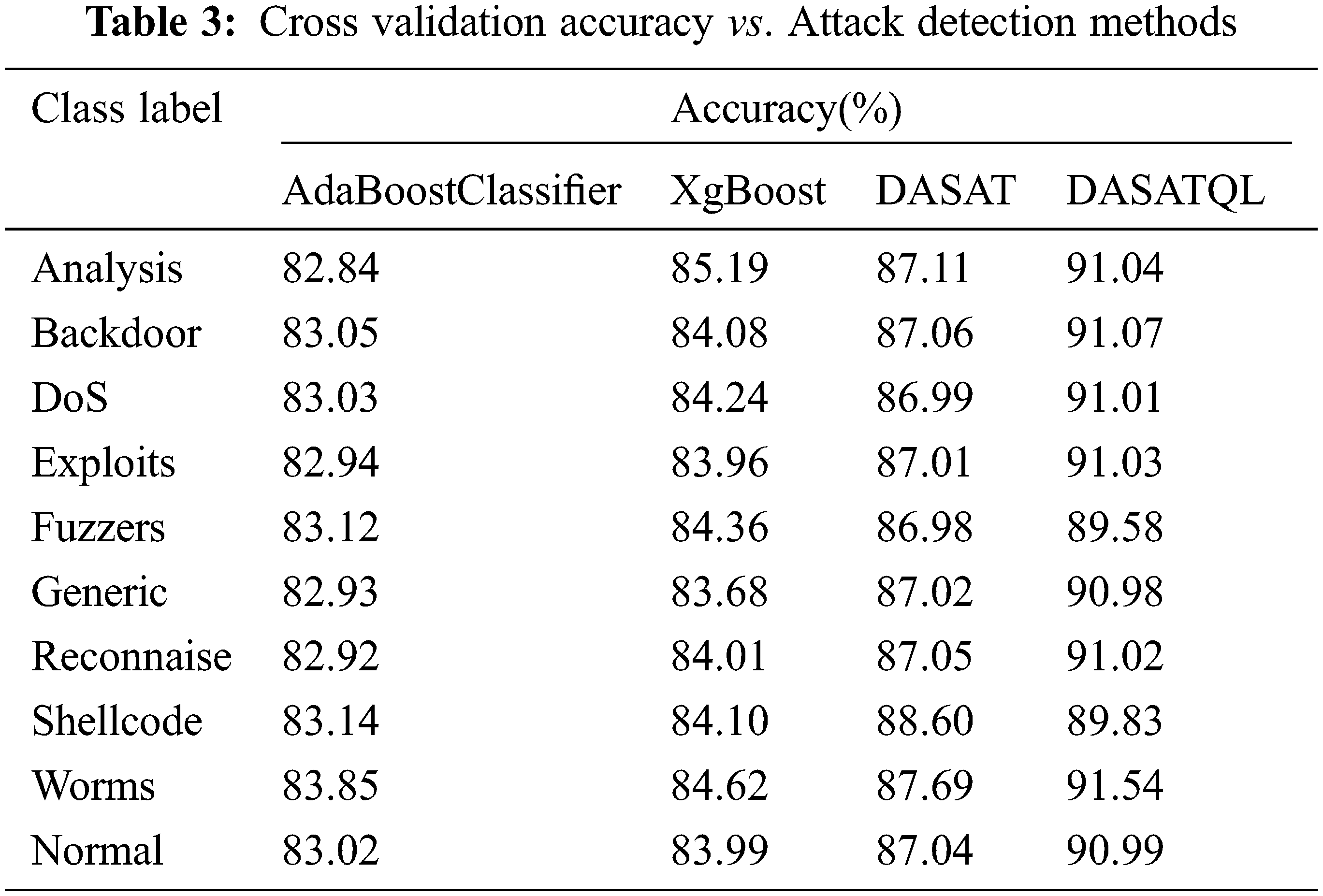
Figure 8: Attack detection methods accuracies for each label

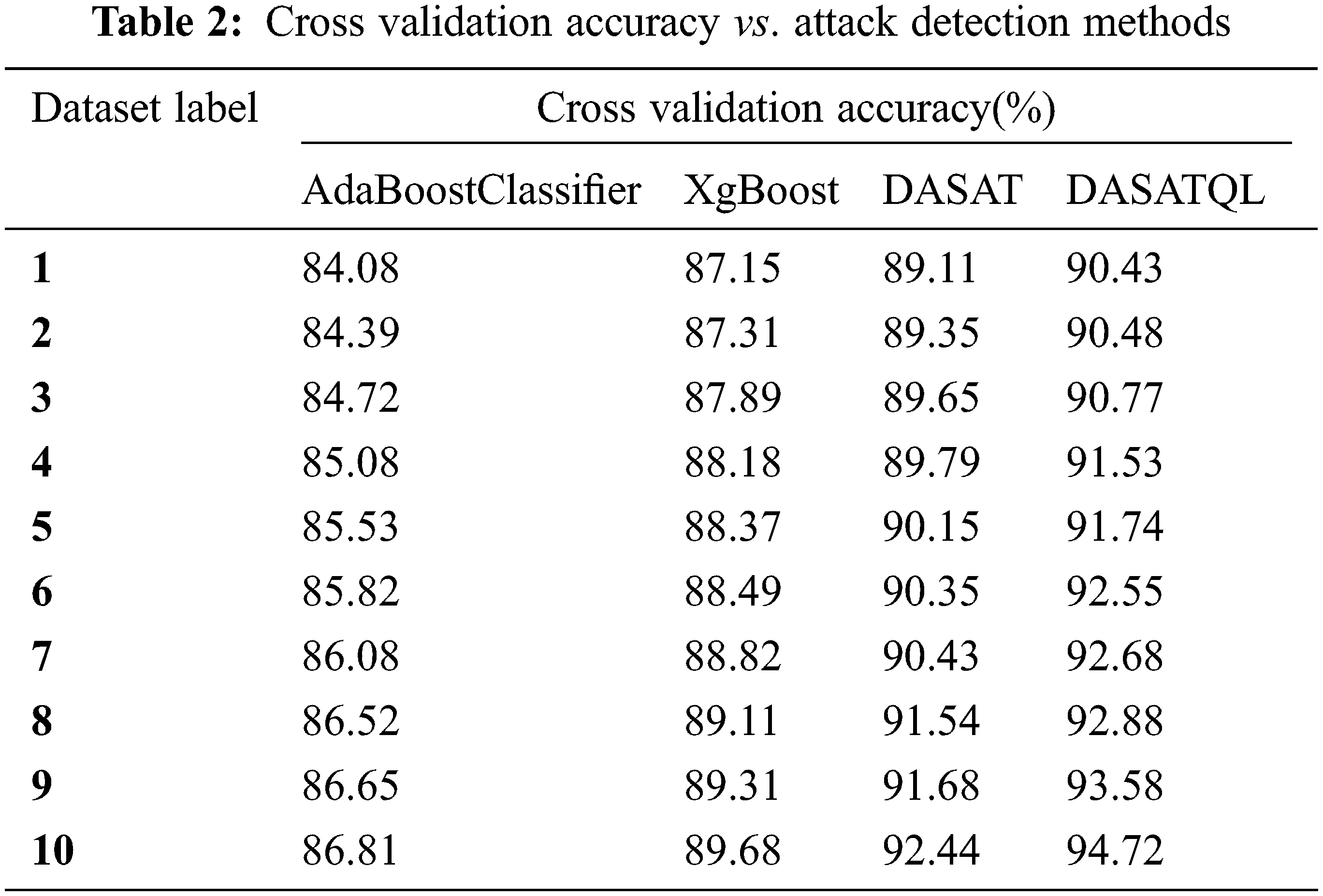
Fig. 8 shows the accuracy comparison results of four classifiers with respect to nine categories of attacks such as Fuzzers, Analysis, Backdoors, DoS, Exploits, Generic, Reconnaissance, Shellcode and Worms. Accuracy of the proposed system is compared with the existing methods for all dataset labels, especially in a dynamic environment. In Fig. 8 its shows that the proposed DASATQL classifier gives higher accuracy of 91.54% for worm attack, whereas other methods such as AdaBoostClassifier, XgBoost, and DASAT gives lesser accuracy of 83.85%, 84.62%, and 87.69% respectively for this attack (See Table 3).

5  Conclusion and Future Work

This research work has combined both supervised and unsupervised MLTs for detecting attacks in the cloud. The proposed work has achieved higher accuracy by its use of multiple classifiers namely SVM, GB and SGD for predicting security attacks. The study has also proposed a new algorithm AKFA for FS from cloud security data. AKFA, based on FA uses major improvements in kernel computations, step size updates and distribution functions to overcome FA’s disadvantages to prove its worthiness in FS when compared to other techniques. The study has also explained requirements of DFS in the context of distributed learning vividly. The proposed addition of a Q learner between FSs and classification acts as an agent to adjust MLTs accuracy results in training/testing of samples. DevQLMLOps model is proposed for automatic selection based on dynamic data evolutions where models scale using Scaling Analyzer and combine via ensemble AdaBoost Classifier. The experimental results have been verified using the metrics of precision, recall, F-measure and accuracy. It can be concluded that the proposed work shows better performance than other classifiers in evaluations. This work aims to add Reinforcement learning model based tool for MLT models in the frame of auto-tuning and auto-selection.

Funding Statement: The authors received no specific funding for this study.

Conflicts of Interest: The authors declare that they have no conflicts of interest to report regarding the present study.

References

1. A. Botta, W. De Donato, V. Persico and E. A. Pescap, “Integration of cloud computing and internet of things: A survey,” Future Generation Computer Systems, vol. 56, no. 7, pp. 684–700, 2016. [Google Scholar]
2. D. F. Ferguson and V. M. Mu, “Journal of grid computing, special issue of cloud computing and services science,” Journal of Grid Computing, vol. 15, no. 2, pp. 139–140, 2017. [Google Scholar]
3. H. J. Syed, A. Gani, R. W. Ahmad, M. K. Khan and A. I. A. Aahmed, “Cloud monitoring: A review, taxonomy, and open research issues,” Journal of Network and Computer Applications, vol. 1, no. 9, pp. 786–797, 2017. [Google Scholar]
4. Z. Li, W. Xie and T. Liu, “Efficient feature selection and classification for microarray data,” PLOS ONE, vol. 13, no. 8, pp. 359–368, 2018. [Google Scholar]
5. D. Jain and V. Singh, “Feature selection and classification systems for chronic disease prediction: A review,” Egyptian Informatics Journal, vol. 19, no. 3, pp. 179–189, 2018. [Google Scholar]
6. S. Mabu, M. Obayashi and T. Kuremoto, “Ensemble learning of rule-based evolutionary algorithm using multi-layer perceptron for supporting decisions in stock trading problems,” Applied Soft Computing, vol. 36, pp. 357–367, 2015. [Google Scholar]
7. E. R. Sparks, A. Talwalkar, D. Haas and M. Franklin, “Automating model search for large scale machine learning,” in Proc. of the Sixth ACM Symp. on Cloud Computing (2015ACM, India, pp. 368–380, 2015. [Google Scholar]
8. M. Wajahat, A. Gandhi, A. Karve and A. Kochut, “Using machine learning for black-box autoscaling,” in 2016 Seventh Int. Green and Sustainable Computing Conf. (IGSC0), USA, pp. 1–8, 2016. [Google Scholar]
9. T. Chen and R. bahsoon, “Survey and taxonomy of self-aware and self-adaptive autoscaling systems in the cloud,” arXiv preprint arXiv:1609.03590, 2016. [Google Scholar]
10. I. Karamitsos, S. Albarhami and C. Apostolopoulos, “Applying devops practices of continuous automation for machine learning,” Information, vol. 11, no. 7, pp. 1–15, 2020. [Google Scholar]
11. A. Truong, A. Walters, J. Goodsitt, K. Hines, C. B. Bruss et al., “Towards automated machine learning: Evaluation and comparison of automl approaches and tools,” 2019 IEEE 31st Int. Conf. on Tools with Artificial Intelligence (ICTAI), vol. 1, pp. 1471–1479, 2019. [Google Scholar]
12. X. Zhang, S. T. Waller and P. Jiang, “An ensemble machine learning-based modeling framework for analysis of traffic crash frequency,” Computer-Aided Civil and Infrastructure Engineering, vol. 35, no. 3, pp. 258–276, 2020. [Google Scholar]
13. A. Nazir and R. A. Khan, “Combinatorial optimization based feature selection method,” A Study on Network Intrusion Detection, pp. 235–249, 2019. [Google Scholar]
14. O. Almomani, “A feature selection model for network intrusion detection system based on pso, gwo, ffa and ga algorithms,” Symmetry, USA, vol. 12, no. 6, pp. 1–20, 2020. [Google Scholar]
15. V. Kumar, D. Sinha, A. K. Das, S. C. Pandey and R. T. Goswami, “An integrated rule based intrusion detection system: Analysis on UNSW-NB15 data set and the real time online dataset,” Cluster Computing, vol. 23, no. 2, pp. 1397–1418, 2020. [Google Scholar]
16. R. R. Karn, P. Kudva and I. A. M. Elfadel, “Dynamic autoselection and autotuning of machine learning models for cloud network analytics,” IEEE Transactions on Parallel and Distributed Systems, vol. 30, no. 5, pp. 1052–1064, 2018. [Google Scholar]
17. UNSW-NB15, “Dataset features and size description,” 2017. Available: https://www.unsw.adfa.edu.au/australiancentre-for-cybersecurity/ [Google Scholar]
18. N. Moustafa and J. Slay, “Unsw-nb15: A comprehensive data set for network intrusion detection systems (unswnb15 network data set),” in Military Communications and Information Systems Conf. (MilCIS), Canberra, ACT, Australia, pp. 1–6, 2015. [Google Scholar]
19. N. Moustafa and J. Slay, “The evaluation of network anomaly detection systems: Statistical analysis of the unsw-nb15 data set and the comparison with the kdd99 data set,” Information Security Journal: A Global Perspective, vol. 25, no. 1–3, pp. 18–31, 2016. [Google Scholar]
20. A. K. Qin, V. L. Huang and P. N. Suganthan, “Differential evolution algorithm with strategy adaptation for global numerical optimization,” IEEE Transactions on Evolutionary Computation, vol. 13, no. 2, pp. 398–417, 2009. [Google Scholar]
21. V. Ho-Huu, T. Nguyen-Thoi, M. H. Nguyen-Thoi and L. le-Anh, “An improved constrained differential evolution using discrete variables (D-ICDE) for layout optimization of truss structures,” Expert Systems with Applications, vol. 42, no. 20, pp. 7057–7069, 2015. [Google Scholar]
22. C. Mu, Q. Zhao, Z. Gao and C. Sun, “Q-learning solution for optimal consensus control of discrete-time multiagent systems using reinforcement learning,” Journal of the Franklin Institute, vol. 356, no. 13, pp. 6946–6967, 2019. [Google Scholar]
23. R. Garreta and G. Moncecchi, Learning scikit-learn: Machine learning in python. Packt Publishing Ltd, Livery Place, Brimingham UK, pp. 1–118, 2013. [Google Scholar]
24. N. H. Sweilam, A. A. Tharwat and N. A. Moniem, “Support vector machine for diagnosis cancer disease: A comparative study,” Egyptian Informatics Journal, vol. 11, no. 2, pp. 81– 92, 2010. [Google Scholar]
25. W. Sun, X. Chen, X. R. Zhang, G. Z. Dai, P. S. Chang et al., “A multi-feature learning model with enhanced local attention for vehicle re-identification,” Computers, Materials & Continua, vol. 69, no. 3, pp. 3549–3560, 2021. [Google Scholar]
26. W. Sun, G. C. Zhang, X. R. Zhang, X. Zhang and N. N. Ge, “Fine-grained vehicle type classification using lightweight convolutional neural network with feature optimization and joint learning strategy,” Multimedia Tools and Applications, vol. 80, no. 20, pp. 30803–30816, 2021. [Google Scholar]
Cite This Article
Copyright © 2023 The Author(s). Published by Tech Science Press.
This work is licensed under a Creative Commons Attribution 4.0 International License , which permits unrestricted use, distribution, and reproduction in any medium, provided the original work is properly cited.
Downloads
Citation Tools