Wind Speed Prediction Using Chicken Swarm Optimization with Deep Learning Model

1  Introduction

Weather conditions certainly affect various aspects of life in modern society. Unfavorable weather conditions and events have direct as well as indirect impacts on a large number of businesses and economic fields, like agriculture, transport, and logistics [1]. Precise and prompt weather predictions are significant for various applications facilitating management and planning related to climatic conditions [2]. Forecasting weather is crucial for predicting natural calamities like hurricanes, extreme rainfall, heat waves, and floods. As wind power has gained significance as a renewable energy over the past few years, wind speed prediction is becoming a prominent tool for productive the effectual and adaptive maintenance of wind parks [3]. However, weather forecasting commonly depends on numerical weather prediction (NWP) techniques for solving complicated arithmetical equations, which pretend thermodynamics and fluids within the natural world’s environment as much as possible [4]. This method needs enormous computational power; with current technological tools and equipment, it may take numerous hours to process. Because of its wide computational requisites, the application of NWP methods is practically limited and restricted to more long-run estimations [5]. Therefore, NWP algorithms are utilized for prediction, for example, 3 h ahead. However, as the time to process this forecast takes more than 3 h, the practical usage of this method is limited. These results become a significant gap for short-run weather forecasting, enabling short-term planning [6].

Through technological development and fortifying advocacy for ecological protection, wind energy production is more commercially competitive than coal-fired power production [7]. As wind power can be directly linked to the wind speed, the volatility and instability of wind speed would cause instability in wind energy production, which has a massive effect on the power grid [8]. To minimize the cost of maintenance caused by system failures and performance degradation, precise forecasting of short-term wind speed is greatly needed. To precisely forecast the wind speed and overcome the uncertainty of its changes, several prediction approaches have been devised over the last decades [9]. As per the forecasting duration and application cases, wind speed prediction is classified into two categories, long-term prediction and short-term prediction. In short-term prediction, the wind speed once every 10 or 20 min or an hour is predicted. In the long-term prediction, the forecast can be made after some days or a month [10]. However, the predicting horizon of long-term forecasting becomes comparatively long, and several unknown elements would affect the forecasting outcomes. Thus, short-term prediction is more versatile and realistic in real applications.

This paper presents an Intelligent Wind Speed Prediction using Chicken Swarm Optimization with Hybrid Deep Learning (IWSP-CSODL) model. The presented IWSP-CSODL model estimates the wind speed using a hybrid deep learning and hyperparameter optimizer. In the presented IWSP-CSODL model, the prediction process is performed via CNN-based long short-term memory with autoencoder (CBLSTMAE) model. To optimally modify the hyperparameters related to the CBLSTMAE model, the CSO algorithm is utilized and thereby reduces the mean square error (MSE). The experimental validation of the IWSP-CSODL model is tested using wind series data under three distinct scenarios.

The remainder of the paper is organized as follows, Section 2 analysis the related works involved in Wind Speed Prediction. Section 3 describes the Proposed Wind Speed Prediction Model and estimates the wind speed using a hybrid deep learning and hyperparameter optimizer. Section 4 then analyses the experimental data and results, including a performance comparison with alternative methodologies. Finally, Section 5 concludes the critical results of the proposed research.

2  Related Works

In Trebing and Mehrkanoon [11], a new paradigm based on a convolutional neural network (CNN) is introduced to predict wind speed. Notably, we have shown that, in contrast to the traditional CNN-based models, the presented method can be able to better characterize the spatio-temporal evolution of the wind dataset by learning the basic structure of the input-output relationship from different views (dimensions) of the input dataset. The suggested technique uses the spatiotemporal multivariate multi-dimensional, past weather dataset to learn novel representations intended for wind prediction. With the information attained from the South African Wind Atlas Project, Daniel et al. [12] addressed the prediction of wind speed, an initial input needed for wind energy generation. Prediction can be performed on two days in advance time horizon. Then, we examine the forecasting efficiency of an artificial neural network (ANN) that is trained by using a decision tree, stochastic gradient boosting (SGB), and Bayesian regularization-based generalized additive models (GAMs).

Lin and Zhang [13] established a new hybrid mechanism that might forecast the upcoming wind speed precisely. At first, the original wind speed duration is decomposed through the fast assembling empirical mode decomposition into different subsets that are additionally incorporated by the run test. The space reconstruction occurs by energetically choosing every incorporated subset input and output vector for the forecasting method. In addition, a better whale optimization algorithm was used for optimizing the weight and bias of the extreme learning machine (ELM) model. The authors in [14] predicted the wind speed at a target station in the north of Iran. The grouping of a multi-layer perceptron (MLP) with a whale optimization algorithm (WOA) was utilized for building a novel model with a restricted amount of information (2004–2014). Next, the MLP-WOA method was applied at every ten target stations, with the tenth station for testing and nine stations for training to improve the performance of the succeeding hybrid mechanism. The ability of the hybrid mechanism in wind speed prediction in every target station was contrasted with MLP improved by the genetic algorithm (GA) called MLP-GA and individual MLP without the WOA optimizer.

Geng et al. [15] developed a wind speed forecasting model with robust integration of principal component analysis (PCA) and long short-term memory (LSTM) networks. Initially, PCA is used to decrease the dimension of the original multi-dimension meteorological information that affects wind speed. Furthermore, a differential evolution (DE) technique is developed for optimizing the learning rate, several hidden layer nodes, and batch size of the LSTM network. Liu et al. [16] implement the industry’s application of the ML method of support vector regression (SVR) and optimization techniques for control variables that can not only reduce energy use and costs. Also fundamentally improve the efficiency of filter press operation. This will open up some possibilities for the intelligent dewatering process and other forms of industrial production optimization. Zhang et al. [17] designed a combined Wind Speed Prediction Model using a convolutional neural network. The work achieved prediction results that have significant advantages in the spatio-temporal features of Wind farms. The disadvantages of the work is utilized limited parameters to measure the performance.

An enhanced deep learning (DL)-based hybrid model for forecasting wind speed is projected in [18]. The new architecture applies stacked LSTM and system architecture evolution (SAE) networks. The SAE extracts abstract and more profound features from the actual wind speed data. An experimental test was performed to identify an optimum stacked LSTM. The feature extracted from SAE is later transported to the optimum stacked LSTM for the wind speed prediction.

3  The Proposed Wind Speed Prediction Model

In this study, a new IWSP-CSODL model has been developed for effectual and precise wind speed forecasting. The presented IWSP-CSODL model estimates the wind speed using a hybrid deep learning and hyperparameter optimizer.

3.1 Level I: CBLSTMAE-Based Prediction Process

In the presented IWSP-CSODL model, the prediction process is performed by the CBLSTMAE model. The architecture encompasses different frameworks comprising 2 CNN layers and an autoencoder (AE) framework composed of a single LSTM layer as a decoder and a CBLSTM as an encoder [19]. The proposed IWSP-CSODL model used hybrid deep learning technique that combine long short-term memory (LSTM) networks, convolutional neural networks (CNN), and autoencoder (AE) are built and tested on wind datasets for wind speed prediction.

Especially, CNN is skilled in extracting complicated features and might save many different unequal trends [20]. Extracting of complicated features decreases the parameters necessary to make the prediction, hence decreasing the network computation when machinating the performance. The feature extraction of CNN and its down-sampling model decreased the computational time, which makes them better suited for the projected applications [21–24]. In this work, the CNN layer receives eight input constraint parameters influencing the forecasting energy consumption, comprising the week indices (bank, holiday, and weekday weekends) and weather conditions (temperature, dew point, and humidity wind speed). They are additionally processed via the hidden layer to generate an output prepared for the AE framework. The output of the CNN layer was given to the input of CBLSTM, which assists as an input to the AE layer [25–28]. Although CNN extracts significant features from datasets, the CBLSTM-AE layer can be used for sequence prediction and data analysis. To reduce the difficulty of the presented framework, a single LSTM is employed in an AE decoder vs. the CBLSTM of the encoder. Furthermore, a single LSTM can learn from temporal dependency from one order to others [29–31]. The encoded data from the output of CBLSTM-AE can be decoded through a single layer of LSTM-AE beforehand, taking place to 2 total connection layers for the final forecasted output. It can be mathematically expressed in the following.

Assume the input vector xim={x1, x2,⋯, xn} , whereby xm indicates the different input vectors, containing weather data, energy consumption, week index, and so on., of m∈M , and n refers to the number of normalized thirty min  units for each observation window, which fed as an input vector xim into CNN layer, the resultant the output is formulated as follows.

yijm=σ(bjm+∑m=1M⁡wm,j1xi+m−1,j0)  (1)

In Eq. (1), yijm denotes output vector xijm of the preceding layer. bjm indicates the bias for j‐th feature maps, m shows the index value of the filter, w indicates the weight of the kernel, and σ denotes the activation function for CNN. Eq. (2) indicates the output vector for k‐th convolution layers. In such case, the next convolution layer in the architecture is equated as

yijm(k)=σ(bjm(k)+∑m=1M⁡wm,jm(k)xi+m−1,j0)  (2)

The pooling layer of the convolution layer samples the activation from mapping features to decrease the parameter count and computational network cost. The max-pooling layer characterized in Eq. (3) uses the maximal values from the preceding layer for its downsampling that assists in adjusting the overfitting model.

Pijm(k)=maxrεR⁡ yi×T+rjk−1  (3)

where y characterizes the pooling size and T denotes stride determining the length of the input dataset.

The output from the maximal pooling layer was given to the input of the BLSTM layer via the gate components. BLSTM comprises dissimilar gates (forget, input, and output gates) in forward and backward directions, and every gate is activated. At the same time, memory cells upgrade the state, characterized as follows in Eqs. (4)–(6) respectively.

it=σ(WpiPi+Whiht−1+Wci⋅ct−1+bi)  (4)

ft=σ(WpfPt+Whfht−1+Wcfct−1+bf)  (5)

0t=σ(WPopt+Whoht−1+WC0⋅ct+b0)  (6)

In the following equation, σ denotes the activation function, b indicates the bias, and ct shows the cell state. Pt indicates the output of the max pooling layer at t time that encompasses the energy utilization dataset and additional parameters utilized as input to AE through the CBLSTM layer. it, ft , and 0t indicates the input, forget, and output gates; correspondingly, ht denotes the hidden state of the BLSTM cell that was upgraded at each t step in backward and forward directions [32–36]. Fig. 1 depicts the infrastructure of the AE technique.

Figure 1: Structure of AE

The cell and hidden states are defined by the gate function of CBLSTM for the hidden and cell states, correspondingly in Eqs. (7) and (8)

ct=ft⋅ct−1+it⋅σ(Wpcpt+Whcht−1+bc)  (7)

ht=0t⋅σ(ct)  (8)

The output of the BLSTM layer was concatenated with backward and forward directions, formulated in Eq. (9).

y^=σ(Wyht→+by)  (9)

The output of BLSTM y^ was given as an input of the LSTM decoder, whereby the resultant output y^=σ(Wyht+by) signifies the input to the two fully connected (FC) dense layers for the last projected output in Eq. (10).

dik=∑j ⁡wjik−1(σ(y^ik−1)+bik−1)  (10)

The CNN layer extracts spatial characteristics from the input dataset, and CBLSTM-AE accepts the feature from a CNN for learning temporal dependency from an estimated output.

3.2 Level II: CSO-Based Hyperparameter Tuning Process

To optimally modify the hyperparameters related to the CBLSTMAE model, the CSO algorithm is utilized and thereby reduces the mean square error (MSE). The CSO approach is preferred over other optimization techniques due to its high parallelism and simplicity [37–40]. The CSO mimics the performance of a chicken swarm and the chicken movement; the CSO is described in the following: CSO contains various groups, and each group has some chicks, hens, and a predominant rooster [41]. The number of chicks, roosters, and hens in the group is established based on the fitness function. The rooster (group head) refers to the chicken that is an optimal fitness value. However, the chick is the chicken that contains the worst fitness value. Most chickens are hens and are arbitrarily chosen to remain in that group. The mother-child and dominance connections in the group stay unchanged and upgraded in the (G) time step. The chicken movement is formulated below is used for rooster updating location given as follows in Eq. (11).

Xijr+1=Xi,jt ∗ (1+randn(0,  σ2))  (11)

where:

σ2={1if fi≤fkexp(fk−fi|fi+ϵ|)Otherwise

where k∈[1,  Nr], k≠i, and Nr denote the rooster count. Xi,j denotes the position of rooster count i in jth dimension at t and t+1 iteration, randn (O,  σ2) generates arbitrary Gaussian number with mean 0 and variance σ2; ϵ indicates the constant with minimal value, and fi indicates the fitness value of the corresponding rooster i. The formula that employs the hen updating position is shown below in Eq. (12).

Xi,jt+1=Xi,jt+S1randn(Xr1,jt−Xi,jt)+S2randn(Xr2,jt−Xi,jt)  (12)

In which, Eq. (13) calculates the  S1

S1=exp⁡(fi−fr1|fi|+ϵ)  (13)

Then replace the  S1 calculation in Eq. (14).

S1= exp (fr2−fi)  (14)

whereas r1, r∈[1,…,N],  r1≠rr denotes the index of the rooster, but r2 indicates the chicken in the swarm hen or rooster, and a uniformly distributed arbitrary value is produced using randn . At last, the formula that applies the chick updating position is given as follows in Eq. (15):

Xi,jt+1=Xi,jt+FL(Xm,jt−Xi,jt),  FL∈[0, 2]  (15)

Now Xm,jt shows the place of i‐th chick mother.

Fig. 2 depicts the flowchart of the CSO technique.

Figure 2: Flowchart of CSO technique

4  Results and Discussion

This section investigates the wind speed prediction outcomes of the IWSP-CSODL model under three distinct scenarios. This proposed work measured the wind speed data of a wind farm, starting from February 1, 2022, to July 30, 2022, with an interval of 3 h, each containing 100 data points in the Kotdwara location. Fig. 3 demonstrates the actual vs. predicted wind speed of the IWSP-CSODL model under scenario 1.

Figure 3: Actual vs. predicted analysis of IWSP-CSODL method under scenario 1

The major hardware requirements are a cloud-based supercomputer, server, virtual machine (VM), several sensors, and meet towers for wind speed prediction. The various sensors are wind speed and direction sensors, humidity sensors, radiation sensors, precipitation sensors, modems, and data loggers. It implied that the IWSP-CSODL model has accurately forecasted the wind speed under all data points. The current work uses climate data information that has been downloaded from the website of https://www.indianclimate.com/show-data.php, and the geographical locations of Kotdwara (a City on Uttarakhand state, India country) have been tabulated in this website.

Fig. 4 illustrates the actual vs. predicted wind speed of the IWSP-CSODL method under scenario 2. It is implicit that the IWSP-CSODL algorithm has precisely forecasted the wind speed under all data points.

Figure 4: Actual vs. predicted analysis of the IWSP-CSODL method under scenario 2

Fig. 5 signifies the actual vs. predicted wind speed of the IWSP-CSODL approach under scenario 3. It represented the IWSP-CSODL technique has accurately forecasted the wind speed under all data points.

Figure 5: Actual vs. predicted analysis of IWSP-CSODL method under scenario 3

Table 1 provides an overall wind speed prediction outcome of the IWSP-CSODL model using scenario 1 [42]. Fig. 6 represents a comparison study of the IWSP-CSODL model with other models under scenario 1. The experimental values ensured the effectual predictive outcomes of the IWSP-CSODL model with minimal values of MSE, Mean Absolute Error (MAE), and Mean Absolute Percentage Error (MAPE) [43–46]. Concerning MSE, the IWSP-CSODL model has offered a lower MSE of 0.5318. In contrast, the Jaya algorithm based-support vector machines (SVM), absolute shrinkage and selection operator (LASSO), Extreme Gradient Boosting (XGBoost) algorithm, Machine learning and pattern recognition (MLPR), deep belief network (DBN), Gaussian processing regression (GPR), Stacked Sparse Auto-Encoder (SSAE), and governance, risk, and compliance (GrC) models have accomplished increased MSE of 0.6492, 0.6508, 0.6699, 0.6769, 0.7032, 0.7094, 0.7159, and 0.8310 respectively. Moreover Concerning, MAE, the IWSP-CSODL algorithm has presented a lower MAE of 0.4967. In contrast, the Jaya-SVM, LASSO, XGBoost, MLPR, DBN, GPR, SSAE, and GrC algorithms have accomplished increased MSE of 0.5899, 0.6089, 0.6203, 0.6215, 0.6236, 0.6385, 0.6505, and 0.6938 correspondingly. At the same time, Concerning MAPE, the IWSP-CSODL technique has offered lower MAPE of 10.1240%, the Jaya-SVM, LASSO, XGBoost, MLPR, DBN, GPR, SSAE, and GrC techniques have accomplished increased MSE of 11.6891%, 12.3410%, 12.7580%, 12.8411%, 12.8487%, 13.0254%, 13.5843%, and 14.3853% correspondingly.

Figure 6: Comparative analysis of IWSP-CSODL approach under scenario 1

A detailed MAPE inspection of the IWSP-CSODL model with recent models for scenario 1 is given in Fig. 7. Here, R2 is the coefficient of determination of the MAPE, scaled between 0 and 1. The IWSP-CSODL model has gained effectual outcomes with a higher R2 value of 0.9687. At the same time, the Jaya-SVM, LASSO, XGBoost, MLPR, DBN, GPR, SSAE, and GrC models have reached reduced R2 values of 0.9468, 0.9428, 0.9413, 0.9204, 0.9116, 0.9064, 0.8927, and 0.8863 respectively.

Figure 7: MAPE analysis of IWSP-CSODL approach under scenario 1

Table 2 provides an overall wind speed prediction outcome of the IWSP-CSODL model in scenario 2. Fig. 8 denotes a comparative study of the IWSP-CSODL model with other models under scenario 2. The experimental values ensured the effectual predictive outcomes of the IWSP-CSODL approach with minimal values of MSE, MAE, and MAPE. Concerning MSE, the IWSP-CSODL algorithm has offered a lower MSE of 1.0114, whereas the Jaya-SVM, LASSO, XGBoost, MLPR, DBN, GPR, SSAE, and GrC approaches have accomplished increased MSE of 1.1309, 1.1523, 1.1550, 1.1704, 1.1784, 1.2027, 1.2036, and 1.4720 correspondingly. In addition, concerning MAE, the IWSP-CSODL model has offered a lower MAE of 0.6834, whereas the Jaya-SVM, LASSO, XGBoost, MLPR, DBN, GPR, SSAE, and GrC models have accomplished increased MSE of 0.7961, 0.8125, 0.8412, 0.8756, 0.8562, 0.8209, 0.8618, and 0.9527 correspondingly. In the meantime, with respect to MAPE, the IWSP-CSODL model has provided lower MAPE of 12.5490, whereas the Jaya-SVM, LASSO, XGBoost, MLPR, DBN, GPR, SSAE, and GrC algorithms have accomplished increased MSE of 15.1714%, 16.2675%, 17.3406%, 15.8917%, 16.3558%, 15.3223%, 15.7527%, and 19.1790% correspondingly.

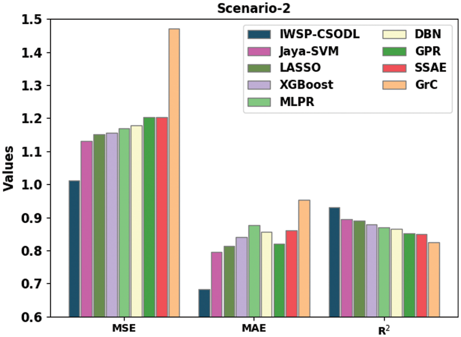
Figure 8: Comparative analysis of IWSP-CSODL approach under scenario 2

A brief MAPE inspection of the IWSP-CSODL approach with current methods on scenario 2 is given in Fig. 9. It demonstrated that the IWSP-CSODL model had obtained effectual outcomes with a higher R2 value of 0.9312 in the MAPE. Meanwhile, the Jaya-SVM, LASSO, XGBoost, MLPR, DBN, GPR, SSAE, and GrC models have reached reduced R2 values of 0.8955, 0.8904, 0.8791, 0.8708, 0.8646, 0.8511, 0.8486, and 0.8246 correspondingly.

Figure 9: MAPE analysis of IWSP-CSODL approach under scenario 2

Table 3 presents the overall wind speed prediction outcomes of the IWSP-CSODL approach on scenario 3. Fig. 10 denotes a comparative study of the IWSP-CSODL approach with other models under scenario 3. The experimental values ensured the effectual predictive outcomes of the IWSP-CSODL model with minimal values of MSE, MAE, and MAPE. With respect to MSE, the IWSP-CSODL model has offered lower MSE of 1.2654, whereas the Jaya-SVM, LASSO, XGBoost, MLPR, DBN, GPR, SSAE, and GrC algorithms have accomplished increased MSE of 1.6437, 1.7420, 1.7547, 1.7670, 1.8035, 1.8051, 1.8115, and 2.4062 correspondingly. Furthermore, concerning MAE, the IWSP-CSODL model has offered a lower MAE of 0.9185, whereas the Jaya-SVM, LASSO, XGBoost, MLPR, DBN, GPR, SSAE, and GrC models have accomplished increased MSE of 1.0179, 1.0124, 1.0714, 1.0584, 1.0431, 1.0214, 1.0667, and 1.2386 respectively. Meanwhile, concerning MAPE, the IWSP-CSODL model has provided a lower MAPE of 16.3842%, whereas the Jaya-SVM, LASSO, XGBoost, MLPR, DBN, GPR, SSAE, and GrC models have accomplished increased MSE of 19.2791%, 18.7221%, 20.2979%, 18.9103%, 18.7322%, 19.9954%, 20.3918%, and 23.5756% correspondingly.

Figure 10: Comparative analysis of IWSP-CSODL approach under scenario 3

A detailed MAPE review of the IWSP-CSODL technique with recent models on scenario 3 is given in Fig. 11. It establishes that the IWSP-CSODL approach has achieved effectual outcomes with a higher R2 value of 0.8432. Meanwhile, the Jaya-SVM, LASSO, XGBoost, MLPR, DBN, GPR, SSAE, and GrC models have reached reduced R2 values of 0.8086, 0.7837, 0.8120, 0.7760, 0.8686, 0.7813, 0.8166, and 0.7025 correspondingly.

Figure 11: MAPE analysis of IWSP-CSODL approach under scenario 3

5  Conclusion

In this study, a new IWSP-CSODL model has been developed for effectual and precise wind speed forecasting. The presented IWSP-CSODL model estimates the wind speed using a hybrid deep learning and hyperparameter optimizer. In the presented IWSP-CSODL model, the CBLSTMAE model performs the prediction process. The CSO algorithm is utilized to optimize the hyperparameters related to the CBLSTMAE model, and thereby reducing MSE. The experimental validation of the IWSP-CSODL model is tested using wind series data under three distinct scenarios. The comparative study pointed out the better outcomes of the IWSP-CSODL model over other recent wind speed prediction models. In the future, the predictive performance of the IWSP-CSODL method could be boosted by the use of hybrid metaheuristic algorithms. The IWSP-CSODL method will be applied for atmospheric pressure prediction.

Acknowledgement: The authors would like to thank the Deanship of Scientific Research at Umm Al-Qura University for supporting this work by Grant Code: (22UQU4281755DSR01).

Funding Statement: This research is funded by Deanship of Scientific Research at Umm Al-Qura University, Grant Code: 22UQU4281755DSR01.

Availability of Data and Materials: Available Based on Request. The datasets generated and/or analyzed during the current study are not publicly available due to the extension of the submitted research work. Still, they are available from the corresponding author on reasonable request.

Conflicts of Interest: The authors declare that they have no conflicts of interest to report regarding the present study.

References

1. S. H. Hur, “Short-term wind speed prediction using extended kalman filter and machine learning,” Energy Reports, vol. 7, no. 1, pp. 1046–1054, 2021. [Google Scholar]

2. V. Bali, A. Kumar and S. Gangwar, “Deep learning based wind speed forecasting-a review,” in Proc. of the 9th Int. Conf. on Cloud Computing, Data Science & Engineering (Confluence), Noida, India, IEEE, pp. 426–431, 2019. [Google Scholar]

3. S. Gangwar, V. Bali and A. Kumar, “Comparative analysis of wind speed forecasting using LSTM and SVM,” EAI Endorsed Transactions on Scalable Information Systems, vol. 7, no. 25, pp. 1–9, 2020. [Google Scholar]

4. M. M. Nezhad, A. Heydari, E. Pirshayan, D. Groppi and D. A. Garcia, “A novel forecasting model for wind speed assessment using sentinel family satellites images and machine learning method,” Renewable Energy, vol. 179, no. 1, pp. 2198–2211, 2021. [Google Scholar]

5. S. Salah, H. R. Alsamamra and J. H. Shoqeir, “Exploring wind speed for energy considerations in eastern Jerusalem-palestine using machine-learning algorithms,” Energies, vol. 15, no. 7, pp. 1–16, 2022. [Google Scholar]

6. P. A. Kulkarni, A. S. Dhoble and P. M. Padole, “Deep neural network-based wind speed forecasting and fatigue analysis of a large composite wind turbine blade,” Journal of Mechanical Engineering Science, vol. 233, no. 8, pp. 2794–2812, 2019. [Google Scholar]

7. D. Lagomarsino-Oneto, G. Meanti, N. Pagliana, A. Verri, A. Mazzino et al., “Physics informed shallow machine learning for wind speed prediction,” arXiv preprint arXiv:2204.00495, 2022. [Google Scholar]

8. H. Demolli, A. S. Dokuz, A. Ecemis and M. Gokcek, “Wind power forecasting based on daily wind speed data using machine learning algorithms,” Energy Conversion and Management, vol. 198, no. 111823, pp. 1–12, 2019. [Google Scholar]

9. Y. Chen, Z. Dong, Y. Wang, J. Su, Z. Han et al., “Short-term wind speed predicting framework based on EEMD-GA-LSTM method under large scaled wind history,” Energy Conversion and Management, vol. 227, no. 113559, pp. 1–16, 2021. [Google Scholar]

10. P. Malik, A. Gehlot, R. Singh, L. R. Gupta and A. K. Thakur, “A review on ANN based model for solar radiation and wind speed prediction with real-time data,” Archives of Computational Methods in Engineering, vol. 29, no. 1, pp. 3183–3201, 2022. [Google Scholar]

11. K. Trebing and S. Mehrkanoon, “Wind speed prediction using multidimensional convolutional neural networks,” in Proc. of the 2020 IEEE Symp. Series on Computational Intelligence (SSCI), Canberra, Australia, IEEE, pp. 713–720, 2020. [Google Scholar]

12. L. O. Daniel, C. Sigauke, C. Chibaya and R. Mbuvha, “Short-term wind speed forecasting using statistical and machine learning methods,” Algorithms, vol. 13, no. 6, pp. 1–30, 2020. [Google Scholar]

13. B. Lin and C. Zhang, “A novel hybrid machine learning model for short-term wind speed prediction in inner Mongolia, China,” Renewable Energy, vol. 179, no. 1, pp. 1565–1577, 2021. [Google Scholar]

14. S. Samadianfard, S. Hashemi, K. Kargar, M. Izadyar, A. Mostafaeipour et al., “Wind speed prediction using a hybrid model of the multi-layer perceptron and whale optimization algorithm,” Energy Reports, vol. 6, no. 1, pp. 1147–1159, 2020. [Google Scholar]

15. D. Geng, H. Zhang and H. Wu, “Short-term wind speed prediction based on principal component analysis and LSTM,” Applied Sciences, vol. 10, no. 13, pp. 1–15, 2020. [Google Scholar]

16. H. Liu and K. You, “Optimization of dewatering process of concentrate pressure filtering by support vector regression,” Scientific Reports, vol. 12, no. 7135, pp. 1–14, 2022. [Google Scholar]

17. J. Zhang, C. Yang, F. Niu, Y. Sun and R. Wang, “Combined wind speed prediction model considering the spatio-temporal features of wind farm,” in Proc. of 2022 2nd Int. Conf. on Computer, Control and Robotics (ICCCR), Shanghai, China, IEEE, pp. 132–138, 2022. [Google Scholar]

18. K. U. Jaseena and B. C. Kovoor, “A hybrid wind speed forecasting model using stacked autoencoder and LSTM,” Journal of Renewable and Sustainable Energy, vol. 12, no. 2, pp. 1–16, 2020. [Google Scholar]

19. P. Park, P. D. Marco, H. Shin and J. Bang, “Fault detection and diagnosis using combined autoencoder and long short-term memory network,” Sensors, vol. 19, no. 21, pp. 1–17, 2019. [Google Scholar]

20. S. S. Alotaibi, E. Alabdulkreem, S. Althahabi, M. A. Hamza, M. Rizwanullah et al., “Artificial fish swarm optimization with deep learning enabled opinion mining approach,” Computer Systems Science and Engineering, vol. 45, no. 1, pp. 737–751, 2023. [Google Scholar]

21. S. Rajendran, O. I. Khalaf, Y. Alotaibi and S. Alghamdi, “MapReduce-Based big data classification model using feature subset selection and hyperparameter tuned deep belief network,” Scientific Reports, vol. 11, no. 1, pp. 1–10, 2021. [Google Scholar]

22. A. M. Shatwan, “Visual pollution and the architecture of façade design: A case study in Jeddah,” Journal of Umm Al-Qura University for Engineering and Architecture, vol. 12, no. 2, pp. 26–29, 2021. [Google Scholar]

23. A. O. Kingsley, R. Surendran and O. I. Khalaf, “Optimal artificial intelligence based automated skin lesion detection and classification model,” Computer Systems Science and Engineering, vol. 44, no. 1, pp. 693–707, 2023. [Google Scholar]

24. H. H. Khan, M. N. Malik, R. Zafar, F. A. Goni, A. G. Chofreh et al., “Challenges for sustainable smart city development: A conceptual framework,” Sustainable Development, vol. 28, no. 5, pp. 1507–1518, 2020. [Google Scholar]

25. T. Tamilvizhi, R. Surendran, C. A. T. Romero and M. Sadish, “Privacy preserving reliable data transmission in cluster based vehicular adhoc networks,” Intelligent Automation & Soft Computing, vol. 34, no. 2, pp. 1265–1279, 2022. [Google Scholar]

26. Z. F. Liu, L. L. Li, M. L. Tseng and M. K. Lim, “Prediction short-term photovoltaic power using improved chicken swarm optimizer-extreme learning machine model,” Journal of Cleaner Production, vol. 248, no. 1, pp. 1–14, 2020. [Google Scholar]

27. M. Liu, Z. Cao, J. Zhang, L. Wang, C. Huang et al., “Short-term wind speed forecasting based on the jaya-SVM model,” International Journal of Electrical Power & Energy Systems, vol. 121, no. 1, pp. 1–9, 2020. [Google Scholar]

28. S. Sennan, D. Pandey, Y. Alotaibi and S. Alghamdi, “A novel convolutional neural networks based spinach classification and recognition system,” Computers, Materials & Continua, vol. 73, no. 1, pp. 343–361, 2022. [Google Scholar]

29. H. S. Gill, O. I. Khalaf, Y. Alotaibi, S. Alghamdi and F. Alassery, “Fruit image classification using deep learning,” Computers, Materials & Continua, vol. 71, no. 3, pp. 5135–5150, 2022. [Google Scholar]

30. T. Tamilvizhi and P. Varthini, “Cessation of overloaded host by increase the inter-migration time in cloud data,” Journal of Theoretical and Applied Information Technology, vol. 95, no. 3, pp. 654–660, 2017. [Google Scholar]

31. Y. Yan, X. Wang, F. Ren, Z. Shao and C. Tian, “Wind speed prediction using a hybrid model of EEMD and LSTM considering seasonal features,” Energy Reports, vol. 8, no. 1, pp. 8965–8980, 2022. [Google Scholar]

32. Q. Wu, H. Zheng, X. Guo and G. Liu, “Promoting wind energy for sustainable development by precise wind speed prediction based on graph neural networks,” Renewable Energy, vol. 199, no. 1, pp. 977–992, 2022. [Google Scholar]

33. R. Ye, S. Feng, X. Li, Y. Ye, B. Zhang et al., “SPLNet: A sequence-to-one learning network with time-variant structure for regional wind speed prediction,” Information Sciences, vol. 609, no. 1, pp. 79–99, 2022. [Google Scholar]

34. Y. Huang, B. Zhang, H. Pang, B. Wang, K. Y. Lee et al., “Spatio-temporal wind speed prediction based on clayton copula function with deep learning fusion,” Renewable Energy, vol. 192, no. 1, pp. 526–536, 2022. [Google Scholar]

35. U. B. Filik, “A new hybrid approach for wind speed prediction using fast block least mean square algorithm and artificial neural network,” Mathematical Problems in Engineering, vol. 2016, no. 8395751, pp. 1–9, 2016. [Google Scholar]

36. H. Wang, M. Xiong, H. Chen and S. Liu, “Multi-step ahead wind speed prediction based on a two-step decomposition technique and prediction model parameter optimization,” Energy Reports, vol. 8, no. 1, pp. 6086–6100, 2022. [Google Scholar]

37. Y. Li, X. Chen, C. Li, G. Tang, Z. Gan et al., “A hybrid deep interval prediction model for wind speed forecasting,” IEEE Access, vol. 9, no. 1, pp. 7323–7335, 2021. [Google Scholar]

38. R. Ye, X. Li, Y. Ye and B. Zhang, “DynamicNet: A time-variant ODE network for multi-step wind speed prediction,” Neural Networks, vol. 152, pp. 118–139, 2022. [Google Scholar] [PubMed]

39. Y. Zhang, H. Sun and Y. Guo, “Wind power prediction based on PSO-SVR and grey combination model,” IEEE Access, vol. 7, no. 1, pp. 136254–136267, 2019. [Google Scholar]

40. G. An, Z. Jiang, X. Cao, Y. Liang, Y. Zhao et al., “Short-term wind power prediction based on particle swarm optimization-extreme learning machine model combined with adaboost algorithm,” IEEE Access, vol. 9, no. 1, pp. 94040–94052, 2021. [Google Scholar]

41. C. Zhang, C. Ji, L. Hua, H. Ma, M. S. Nazir et al., “Evolutionary quantile regression gated recurrent unit network based on variational mode decomposition, improved whale optimization algorithm for probabilistic short-term wind speed prediction,” Renewable Energy, vol. 197, no. 1, pp. 668–682, 2022. [Google Scholar]

42. Z. Sun, H. Sun and J. Zhang, “Multistep wind speed and wind power prediction based on a predictive deep belief network and an optimized random forest,” Mathematical Problems in Engineering, vol. 2018, no. 6231745, pp. 1–15, 2018. [Google Scholar]

43. J. Jin, B. Wang, M. Yu, J. Liu and W. Wang, “A novel self-adaptive wind speed prediction model considering atmospheric motion and fractal feature,” IEEE Access, vol. 8, no. 1, pp. 215892–215903, 2020. [Google Scholar]

44. Y. Nie, H. Bo, W. Zhang and H. Zhang, “Research on hybrid wind speed prediction system based on artificial intelligence and double prediction scheme,” Complexity, vol. 2020, no. 9601763, pp. 1–22, 2020. [Google Scholar]

45. Z. Tian and J. Wang, “A novel wind speed interval prediction system based on neural network and multi-objective grasshopper optimization,” International Transactions on Electrical Energy Systems, vol. 2022, no. 5823656, pp. 1–23, 2022. [Google Scholar]

46. W. Hu, Q. Yang, P. Zhang, Z. Yuan, H. Chen et al., “A novel two-stage data-driven model for ultra-short-term wind speed prediction,” Energy Reports, vol. 8, no. 1, pp. 9467–9480, 2022. [Google Scholar]