Statistical Data Mining with Slime Mould Optimization for Intelligent Rainfall Classification

1  Introduction

Data mining represents extracting or mining knowledge from massive quantities of data. In other words, data mining is the science, art, and technology of discovering huge and complex bodies of data for beneficial patterns. Practitioners and Theoreticians are constantly searching for more appropriate approaches to make the process accurate, more efficient, and cost-effective [1]. The statistical data mining (SDM) technique is established for effectively processing massive quantities of data that are usually multi-dimensional and probably of many complex types [2]. Some traditional statistical methods for data analysis, particularly for numerical data. This method has been extensively used for scientific records (viz., records from experiments in manufacturing, physics, engineering, medicine, and psychology) and data from the social sciences and economics. Rainfall prediction remains a serious concern and has drawn the consideration of industries, governments, the scientific community, and risk management entities [3]. Rainfall is a climatic factor that affects several human events, such as construction, agricultural production, forestry and tourism, and power generation, amongst others [4]. In that regard, rainfall prediction is crucial since this parameter has the maximum correlation with adversarial natural disasters like flooding, landslides, avalanches, and mass movements. This incident has adversely impacted society in recent years. As a result, having an improved technique for rainfall prediction could allow taking mitigation and preventive measures for these natural phenomena [5].

Besides, this prediction facilitates the supervision of construction, agriculture activities, transport, health, and tourism, amongst others [6]. For events accountable for disaster prevention, providing precise meteorological prediction helps decision-making despite the probable occurrence of natural events [7]. To achieve this prediction, there exist different methodologies, which ranges from naive method to those that use complicated approaches like artificial intelligence (AI), and artificial neural network (ANN), has been the most attractive and valuable approaches for the prediction task [8]. ANN, vs. conventional approaches in meteorology, depends on a self-adaptive mechanism that learns from examples and captures functional relationships amongst data. However, the relationship still needs to be determined or explained [9]. Recently, the Deep Learning (DL) algorithm has been used as an effective method in ANN for resolving difficult challenges. DL is a common term used to represent a sequence of multi-layer architecture that can be trained using unsupervised algorithms [10]. The major development is learning a valid, non-linear, and compact presentation of data through unsupervised methods, hoping that the novel data presentation contributed to the prediction technique.

Suparta et al. [11] intend to forecast rainfall by exploring the implementation of AI methods like Adaptive NeuroFuzzy Inference System (ANFIS). The modelled approach compiles NN learning capabilities having transparent linguistic representations of fuzzy systems. The ANFIS approach has several input structures and membership functions tested, constructed, and trained to evaluate the model’s ability. Dada et al. [12] presented 4 non-linear approaches like Artificial Neural Networks (ANN) for predicting rainfall. ANN is capable of mapping various output and input patterns. The Elman Neural Network (ENN), FFNN, RNN, and Cascade Forward Neural Network (CFNN) are employed for rainfall prediction. Wang et al. [13] inspect the applicability of numerous predicting methods based on wavelet packet decomposition (WPD) in the annual prediction of rainfall, and a novel hybrid precipitation prediction structure (WPD-ELM) was devised with WPD and ELM. These works are described as follows: WPD can be employed for decomposing creative precipitation data into numerous sublayers; ELM method, BPNN, and ARIMA were used to realize the decomposed sequences’ forecasting computation.

Manoj et al. [14] modelled the rainfall predictive method related to the DL network, the convolutional LSTM (convLSTM) method that promises to forecast related to the spatial-and-temporal paradigms. The convLSTM weights were fine-tuned utilizing the projected Salp-stochastic gradient descent algorithm (S-SGD) that can be the amalgamation of the Salp swarm algorithm (SSA) presented in stochastic gradient descent (SGD) approach for facilitating the global fine-tuning of the weights and for assuring a superior predictive accuracy. In contrast, the formulated DL structure can be constructed in the MapReduce structure, allowing the potential big data management. Liyew et al. [15] study was to find the related atmospheric features which might cause rainfall and forecast the intensity of daily rainfall utilizing ML approaches. The Pearson correlation method has been utilized for selecting related environmental parameters employed as input for the ML approach. The dataset has been gathered for measuring the performances of 3 ML methods (Extreme Gradient Boost (XGBoost), Multivariate Linear Regression, and Random Forest (RF)).

This paper introduces an effective statistical Data Mining for Intelligent Rainfall Prediction using Slime Mould Optimization with Deep Learning (SDMIRP-SMODL) model. In the presented SDMIRP-SMODL model, the feature subset selection process is performed by the SMO algorithm, which in turn minimizes the computation complexity. For rainfall prediction. Convolution neural network with long short-term memory (CNN-LSTM) approach is exploited. At last, this study involves the pelican optimization algorithm (POA) as a hyperparameter optimizer. A wide-ranging simulation analysis was executed to highlight the betterment of the SDMIRP-SMODL model. The comparative outcomes reported the supremacy of the SDMIRP-SMODL model compared to existing techniques.

2  The Proposed Rainfall Prediction Model

This study established a new SDMIRP-SMODL system for rainfall prediction systems. The SDMIRP-SMODL technique comprises SMO based on feature subset selection, CNN-LSTM prediction, and POA hyperparameter tuning. Fig. 1 illustrates the overall process of the SDMIRP-SMODL approach.

Figure 1: Overall process of the PODTL-BIR approach

2.1 SMO-Based Feature Selection

In the presented SDMIRP-SMODL method, the feature subset selection process was performed by the SMO algorithm. The projected SMO encompasses many distinctive characteristics involving mathematical modelling, which employs adaptive weight to mimic the procedure of generating positive and negative feedback in slime mold propagative waves [16]. The feature depends on a bio-oscillator, creating the optimal pathway to interconnect food with highly exploring capability and exploitation tendency. A summary of the SMO algorithm is shown as follows:

Approach Food: The following rules are provided to characterize the behaviour of SM as an arithmetical formula for replicating the contraction method:

X(t+1)→={Xb(t)→+vb→. (W⟶⋅XA(t)→−XB(t)→), r<p vc⟶⋅X(t)→, r≥p (1)

In Eq. (1), W⟶ indicates the weight of SM, and v→b denotes a variable within [−a, a], vc⟶ linearly reduces from [0, 1]. t characterizes the current iteration, Xb⟶ characterizes the different positions with the maximum odor smell, X embodies the SM position, XA⟶ and XB⟶ characterize two individuals arbitrarily chosen from the swarm, and W⟶ denotes the SM weight. The formulation of p is shown below:

p=tanh|S(i)−DF|(2)

where i∈1,2,…,n, S(i) signifies fitness of X⟶. The optimal fitness attained in every iteration is represented as the DF. And it is given in the following:

vb⟶=[−a,a],(3)

a=arctanh (−(tmax−t)+1),(4)

The equation of W⟶ is represented in the following:

W(SmellIndex(i))→={1+r⋅log(bF−S(i)bF−wF+1), condition 1−r⋅log(bF−S(i)bF−wF+1), others(5)

Smell Index=sort(S)(6)

Now, the condition signifies that S(i) ranks the initial half of the population, r symbolizes the arbitrary integer within [0,1], and bF and wF signify the optimum and worst fitness attained in the existing iteration method, correspondingly. The smell Index characterizes the series of fitness values arranged.

Wrap Food: The subsequent defines the updating location of SM:

X∗→={rand .(UB−LB)+LB, rand<zXb(t)→+vb⟶⋅(W⋅XA(t)→−XB(t)→),r<pvc⟶⋅X(t)→, r≥p(7)

Here LB and UB characterize the lower and upper limits, and rand and r represent the arbitrary number in [0,1].

Grabble Food: As the iteration count rises, the value of vb→ oscillates arbitrarily within [−a, a] and eventually tends to zero. The value of vc→ oscillates amongst [1, 1] and progressively approaches zero.

The fitness function (FF) employed from the SMO system is to contain a balance amongst the count of particular features from every solution (min) and classifier accuracy (max) attained by employing these chosen features, Eq. (8) signifies the FF for measuring solutions.

Fitness=αγR(D)+β|R||C|(8)

where γR(D) denotes the classifier error rate of the presented classification. |R| stands for the cardinality of chosen subset, and |C| signifies the entire amount of features from the dataset α and β are 2 parameters equivalent to the significance of classifier quality and subset length. ∈ [1, 0] and β=1−α.

2.2 CNN-LSTM-Based Rainfall Prediction

In this work, the CNN-LSTM model is exploited to predict rainfall. Long short-term memory is the development of recurrent neural networks (RNN) [17]. LSTM presents a memory block instead of a traditional RNN unit to overcome gradient exploding and vanishing problems. Then, a cell state is added to store the long-term state, that is, its major dissimilarity from RNN. An LSTM connects and remembers preceding data to the dataset attained in the present. LSTM is coupled with 3 gates. Namely, input, forget, and output gates, whereby χt represent the existing inputs; Ct and Ct−1 denote the previous and new cell states, correspondingly; and ht and ht−1 indicate the current and preceding outputs, correspondingly. The standard of input gates of LSTM is presented in the succeeding formula.

it=σ(Wi⋅[ht−1)xt]+bi)(9)

C~=tanh(Wi⋅[ht−1, xt]+bi)(10)

Ct=ftCt−1+itc~t(11)

For passing ht−1 and χt via a sigmoid layer for deciding where part of the dataset needs to be appended using Eq. (9). Consequently, to achieve novel data afterwards, ht−1 and χt are passed by the tanh layer using (10). The present moment dataset, C~ and long-term memory dataset Ct−1 into Ct are integrated with (11), Wi represents a sigmoid output, and Ct~ denotes a tanh output. Now, Wi represents the weight matrix, and bi epitomizes the input gate bias of LSTM. Next, the LSTM forget gate enables data extraction using a dot product and a sigmoid layer. Eq. (12) is used to decide whether forgetting a relevant dataset from a primary cell with a specific probability is implemented. Wf denotes the weight matrix, bf represents the offset, and σ characterizes the sigmoid operation.

ft=σ(Wf⋅[ht−1)xt]+bf)(12)

The LSTM output gate determines the state essential for continuance by ht−1 and χt inputs. The concluding output is attained and multiplied with the state decision vector that passes novel Ct data via the tanh layer.

Ot=σ(Wo⋅[ht−1,xt]+bo)(13)

ht=Ottanh(Ct)(14)

From the expression, bo and Wo correspondingly, the LSTM bias and output gate weighted matrices. Fig. 2 demonstrates the structure of CNN-LSTM.

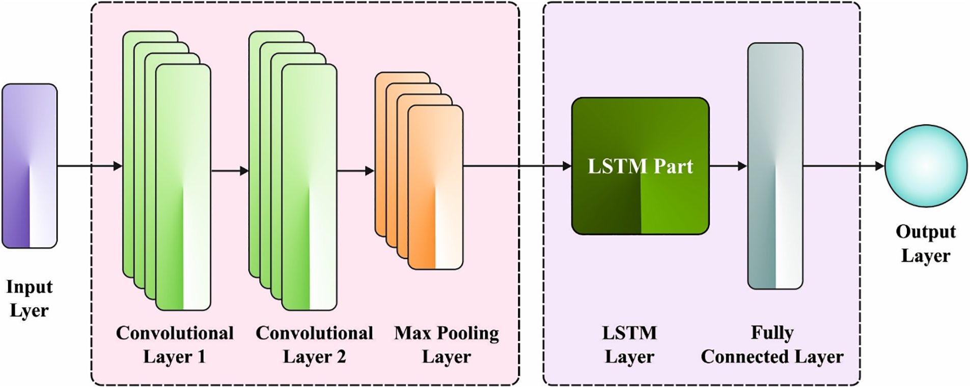
Figure 2: Structure of CNN-LSTM

An integrated approach has been intended for automatic rainfall detection and combining LSTM and CNN networks from which the CNN is applied to extract complicated features from an image. LSTM is also employed as a classification. The network has twenty layers: 1 LSTM layer, 1 FC layer, 5 pooling layers, twelve convolution layers, and 1 output layer using the softmax operation. Every convolutional block is integrated into 1 pooling layer and multiple 2D-CNNs. Subsequently, a dropout layer is considered a twenty-five percent dropout rate. A size of 3× 3 convolution kernel layers is exploited to extract features activated through the ReLU operation. The max− pooling function with a size of 2×2 convolution layers is applied to reduce the dimension of the input image. In the final portion, the mapping function is transported to the LSTM for extracting time data. Afterwards, the convolution blocks, the output form, are considered as (none, 7, 7, and 512).

2.3 POA-Based Hyperparameter Tuning

At the final stage, the POA as a hyperparameter optimizer of the CNN-LSTM model helps enhance classification output. POA is a population-based methodology whereby the pelican is a member of the population [18]. In this work, every population member implies a solution candidate. All the population members propose a value for the optimization variable along with the location of the problem. Initially, the population member is initialized randomly, as stated by the lower and upper bounds of the searching domain,

xi,j=lj+rand⋅(uj−lj), i=1,2,…, N, j=1,2,…,m,(15)

In Eq. (15), xi,j indicates the value of the j-th parameter specified by the i-th solution candidate, N indicates population member count, m illustrates the parameter number, rand indicates an arbitrary integer within [0, 1], lj and uj show the j-th lower, and j-th upper bounds in the search space. The population member of pelicans in the projected POA is recognized by a matrix named population matrix in Eq. (16). The matrix column signifies the suggested value in the search space. In contrast, every row of the matrix characterizes a solution candidate.

X=[X1⋮Xi⋮XN]N×m=[χ1^{'}1…χ1^{'}j…χ1^{'}m⋮⋱⋮ ⋮χi^{'}1…χi^{'}j…χi^{'}m⋮ ⋮⋱⋮xN^{'}1⋯xN,j…xN,m]N×m(16)

In Eq. (16), X indicates the population matrix of pelicans, and Xi shows the i-th pelican.

In this work, all the population members are a pelican whose solution candidate is given to the problem. As a result, an objective function is measured according to the solution candidate. The value attained for the objective function is defined by the vector named objective function vector, as given below.

F=[F1⋮Fi⋮FN]N×1=[F(X1) ⋮F(Xi) ⋮F(XN)]N×1(17)

In Eq. (17), F indicates the objective function vector, and Fi represents the objective function value of the i-th solution candidate [19,20].

The projected approach simulates the strategy and behavior of pelicans while hunting and attacking targets to upgrade the solution candidate, and it can be given in the following steps:

 i.   Moving to the target (exploration stage).

ii.   Flying on the water surface (exploitation stage).

Afterwards, each population member has been upgraded according to the first and second stages according to the original status of the population and values of an objective function, and the optimal candidate solution would be upgraded. Lastly, the optimal solution candidate is characterized by a quasi-optimum solution in the search space.

3  Results and Discussion

The SDMIRP-SMODL approach is simulated utilizing Python 3.6.5 on PC i5-8600k, 1TB HDD, GeForce 1050Ti 4 GB, 250 GB SSD, and 16 GB RAM. The following are the parameter settings: learning rate: 0.01, dropout: 0.5, batch size: 5, activation: ReLU and epoch count: 50. The experimental evaluation of the SDMIRP-SMODL approach is tested utilizing a dataset comprising 23682 instances in the negative class and 1865 instances in the positive class, as depicted in Table 1. The dataset holds 18 features, and the proposed model has chosen a set of 12 features. The dataset is split into 70:30 and 80:20 training (TR) and testing (TS) data for experimental validation.

The confusion matrix produced by the SDMIRP-SMODL system under varying training set (TRS) and testing set (TSS) data is given in Fig. 3. On 80% of the TRS, the SDMIRP-SMODL technique has identified 18619 instances into negative class and 1082 instances into positive class. Meanwhile, on 20% of TSS, the SDMIRP-SMODL approach identified 4645 instances as negative and 294 as positive classes. Eventually, on 70% of TRS, the SDMIRP-SMODL approach identified 16369 instances as negative and 926 as positive classes. At last, on 30% of the TSS, the SDMIRP-SMODL methodology has identified 7046 instances as a negative class and 399 as a positive class.

Figure 3: Confusion matrix of SDMIRP-SMODL methodology (a) 80% of TRS, (b) 20% of TSS,(c) 70% of TRS, and (d) 30% of TSS

Table 2 provides an overall classification outcome of the SDMIRP-SMODL approach with 80:20 of TRS/TSS.

Fig. 4 reports the rainfall classification outcome of the SDMIRP-SMODL model on 80% of the TRS. The SDMIRP-SMODL method has recognized negative samples with accuy, precn, recal, specy, and ER of 96.40%, 97.97%, 98.19%, 73.41%, and 3.60%, respectively. Also, the SDMIRP-SMODL model has categorized positive samples with accuy, precn, recal, specy, and ER of 96.40%, 75.88%, 73.41%, 98.19%, and 3.60%, respectively. Besides, the SDMIRP-SMODL model has obtained average accuy, precn, recal, specy, and ER of 96.40%, 86.91%, 85.80%, 85.80%, and 3.60%, respectively.

Figure 4: Result analysis of SDMIRP-SMODL method on 80% of TR data

Fig. 5 demonstrates a detailed classification outcome of the SDMIRP-SMODL model on 20% of TSS. The SDMIRP-SMODL algorithm has recognized negative samples with accuy, precn, recal, specy, and ER of 96.65%, 97.95%, 98.43%, 75.19%, and 3.35% correspondingly. Also, the SDMIRP-SMODL system has categorized positive samples with accuy, precn, recal, specy, and ER of 96.65%, 79.89%, 75.19%, 98.43%, and 3.35%, respectively. Moreover, the SDMIRP-SMODL methodology has achieved average accuy, precn, recal, specy, and ER of 96.65%, 88.92%, 86.81%, 86.81%, and 3.35%, correspondingly.

Figure 5: Rainfall classification results of SDMIRP-SMODL approach under 20% of the TSS

Table 3 offers an overall classification outcome of the SDMIRP-SMODL technique with a 70:30 TRS/TSS.

Fig. 6 depict a brief classification outcome of the SDMIRP-SMODL method on 70% of the TRS. The SDMIRP-SMODL methodology has recognized negative samples with accuy, precn, recal, specy, and ER of 96.72%, 97.61%, 98.88%, 69.78%, and 3.28%, respectively. The SDMIRP-SMODL approach has categorized positive samples with accuy, precn, recal, specy, and ER of 96.72%, 83.27%, 69.78%, 98.88%, and 3.28% correspondingly. In addition, the SDMIRP-SMODL technique has obtained average accuy, precn, recal, specy, and ER of 96.72%, 90.44%, 84.33%, 84.33%, and 3.28% correspondingly.

Figure 6: Rainfall classification results of SDMIRP-SMODL system on 70% of TR data

Fig. 7 showcases a detailed classification outcome of the SDMIRP-SMODL approach on 30% of TSS. The SDMIRP-SMODL model has recognized negative samples with accuy, precn, recal, specy, and ER of 97.13%, 98.07%, 98.86%, 74.16%, and 2.87% correspondingly. Simultaneously, the SDMIRP-SMODL technique has categorized positive samples with accuy, precn, recal, specy, and ER of 97.13%, 83.13%, 74.16%, 98.86%, and 2.87%, respectively. Moreover, the SDMIRP-SMODL algorithm has gained average accuy, precn, recal, specy, and ER of 97.13%, 90.60%, 86.51%, 86.51%, and 2.87%, correspondingly.

Figure 7: Rainfall classification results of SDMIRP-SMODL system on 30% of the TS database

The training accuracy (TRAY) and validation accuracy (VLAY) achieved by the SDMIRP-SMODL technique on the TSS is illustrated in Fig. 8. The results revealed that the SDMIRP-SMODL approach had achieved superior values of TRAY and VLAY. Mostly the VLAY appeared greater than TRAY.

Figure 8: TRAY and VLAY study of SDMIRP-SMODL methodology

The training loss (TRLS) and validation loss (VLLS) executed by the SDMIRP-SMODL approach on the TSS are shown in Fig. 9. The experimental result stated that the SDMIRP-SMODL technique had realized lower values of TRLS and VLLS. The VLLS is lesser than TRLS.

Figure 9: TRLS and VLLS study of SDMIRP-SMODL methodology

A clear precn−recal study of the SDMIRP-SMODL methodology on the TSS is revealed in Fig. 10. The obtained result exposed that the SDMIRP-SMODL technique has improved precn−recal values under every class.

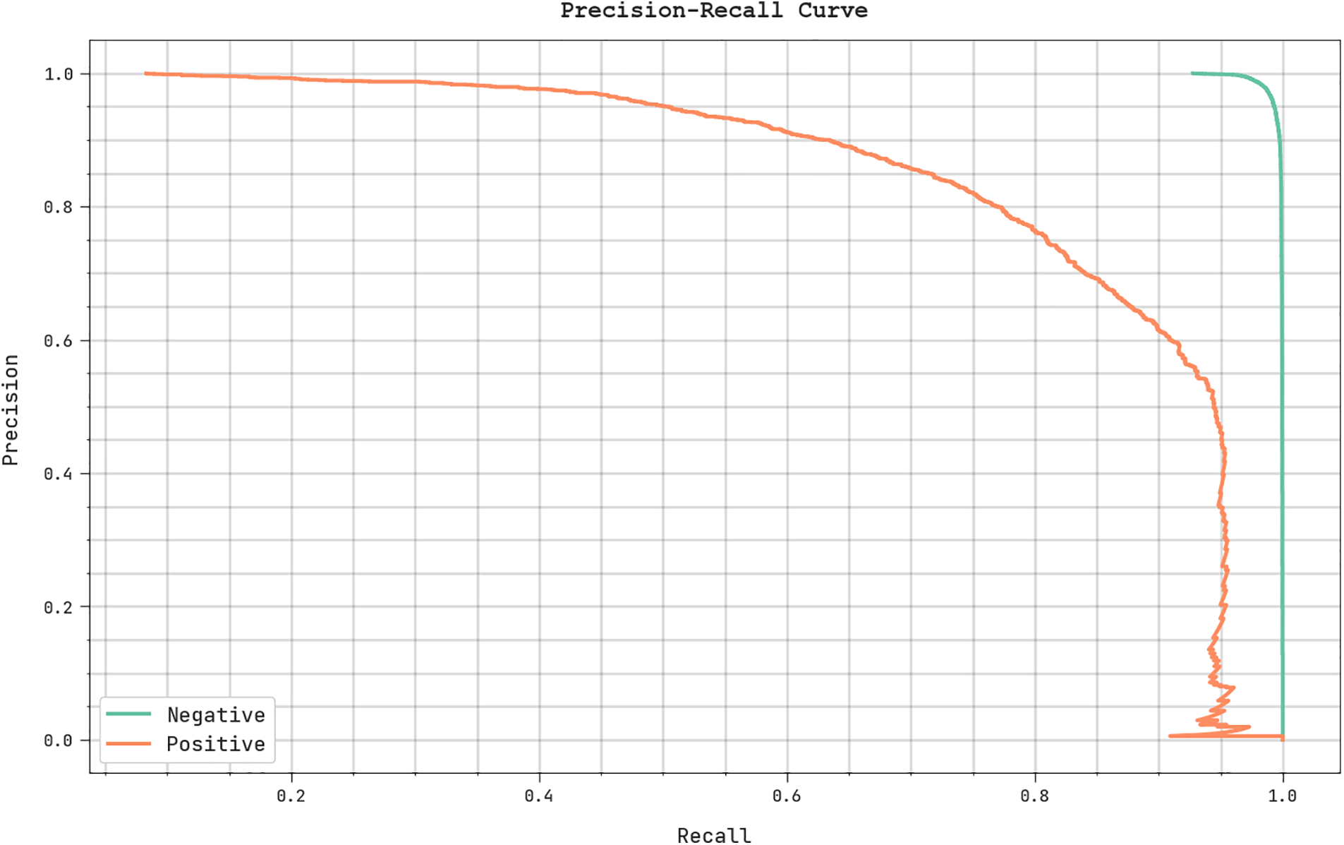
Figure 10: Precn−recal study of SDMIRP-SMODL approach

A brief ROC analysis of the SDMIRP-SMODL system on the TSS is illustrated in Fig. 11. The outcome revealed the SDMIRP-SMODL approach had presented its ability to categorize several classes on TSS.

Figure 11: ROC study of SDMIRP-SMODL approach

Table 4 provides a detailed accuracy and miss rate analysis of the SDMIRP-SMODL system with recent models. Fig. 12 provides an accurate comparative rate (ACR) analysis of the SDMIRP-SMODL system with contemporary techniques. The results implied that the DTSLIQ, NV, and PRNN-10 Neuron models had poor performance with lower ACR values of 72.21%, 78.55%, and 82.3%, respectively. Next, the INBC and Bayesian approaches have shown slightly enhanced ACR values of 90.17% and 90.93%, correspondingly. Likewise, the DT and SVM methods have reported reasonable ACR values of 91% and 92%, respectively. Though the fused ML model has accomplished a considerable ACR value of 94.22%, the SDMIRP-SMODL system has outperformed higher performance with a maximal ACR of 97.13%.

Figure 12: ACR analysis of SDMIRP-SMODL approach with existing methodologies

Fig. 13 offers a comparative miss rate (MSR) inspection of the SDMIRP-SMODL approach with recent algorithms. The outcomes revealed that the DTSLIQ, NV, and PRNN-10 Neuron techniques had worse performance with higher MSR values of 27.79%, 21.45%, and 17.7%, respectively. Next, the INBC and Bayesian methods have exhibited somewhat enhanced MSR values of 9.83% and 9.07%, respectively. Similarly, the DT and SVM techniques have correspondingly obtained reasonable MSR values of 9% and 8%. But, the fused ML system has accomplished a considerable MSR value of 5.78%, and the SDMIRP-SMODL approach has demonstrated higher performance with a lesser MSR of 2.87%.

Figure 13: MSR analysis of SDMIRP-SMODL approach with existing methodologies

From these discussions, it can be assured that the SDMIRP-SMODL technique has shown improved performance over other models.

4  Conclusion

This study established a new SDMIRP-SMODL system for rainfall prediction systems. The SDMIRP-SMODL technique comprises SMO based on feature subset selection, CNN-LSTM prediction, and POA hyperparameter tuning. In the presented SDMIRP-SMODL algorithm, the feature subset selection process is performed by the SMO algorithm, which minimizes the computation complexity. At the same time, the POA, as a hyperparameter optimizer of the CNN-LSTM model, helps accomplish enhanced classification output. A wide-ranging simulation analysis was applied to highlight the betterment of the SDMIRP-SMODL approach, and the comparative outcomes reported the supremacy of the SDMIRP-SMODL model compared to existing techniques with maximum accuracy of 97.13%. In the future, the presented model will be extended to the design of ensemble learning-based classification models with optimal clustering techniques.

Funding Statement: This research was partly supported by the Technology Development Program of MSS [No. S3033853] and by the National Research Foundation of Korea (NRF) grant funded by the Korea government (MSIT) (No. 2021R1A4A1031509).

Conflicts of Interest: The authors declare that they have no conflicts of interest to report regarding the present study.

References

1. J. Refonaa, M. Lakshmi, S. Dhamodaran, S. Teja and T. N. M. Pradeep, “Machine learning techniques for rainfall prediction using neural network,” Journal of Computational and Theoretical Nanoscience, vol. 16, no. 8, pp. 3319–3323, 2019. [Google Scholar]

2. A. Azizah, R. Welastika, A. N. Falah, B. N. Ruchjana and A. S. Abdullah, “An application of markov chain for predicting rainfall data at west java using data mining approach,” IOP Conference Series: Earth and Environmental Science, vol. 303, pp. 012026, 2019. [Google Scholar]

3. K. Kar, N. Thakur and P. Sanghvi, “Prediction of rainfall using fuzzy dataset,” International Journal of Computer Science and Mobile Computing, vol. 8, no. 4, pp. 182–186, 2019. [Google Scholar]

4. R. A. Colomo, D. C. Nieves and M. Méndez, “Comparative analysis of rainfall prediction models using machine learning in islands with complex orography: Tenerife island,” Applied Sciences, vol. 9, no. 22, pp. 4931, 2019. [Google Scholar]

5. S. Manandhar, S. Dev, Y. H. Lee, Y. S. Meng and S. Winkler, “A data-driven approach for accurate rainfall prediction,” IEEE Transactions on Geoscience and Remote Sensing, vol. 57, no. 11, pp. 9323–9331, 2019. [Google Scholar]

6. M. Chhetri, S. Kumar, P. P. Roy and B. G. Kim, “Deep BLSTM-GRU model for monthly rainfall prediction: A case study of Simtokha, Bhutan,” Remote Sensing, vol. 12, no. 19, pp. 1–13, 2020. [Google Scholar]

7. M. I. Khan and R. Maity, “Hybrid deep learning approach for multi-step-ahead daily rainfall prediction using gcm simulations,” IEEE Access, vol. 8, pp. 52774–52784, 2020. [Google Scholar]

8. C. Chen, C. Zhang, Q. Kashani, M. H. Jun, C. Bateni et al., “Forecast of rainfall distribution based on fixed sliding window long short-term memory,” Engineering Applications of Computational Fluid Mechanics, vol. 16, no. 1, pp. 248–261, 2022. [Google Scholar]

9. A. Rahman, S. Abbas, M. Gollapalli, R. Ahmed, S. Aftab et al., “Rainfall prediction system using machine learning fusion for smart cities,” Sensors, vol. 22, no. 9, pp. 3504, 2022. [Google Scholar] [PubMed]

10. I. Saputra and D. A. Kristiyanti, “Application of data mining for rainfall prediction classification in Australia with decision tree algorithm and c5. 0 algorithm,” Seminar Nasional Informatika (SEMNASIF), vol. 1, no. 1, pp. 71–87, 2021. [Google Scholar]

11. W. Suparta and A. A. Samah, “Rainfall prediction by using ANFIS times series technique in South Tangerang, Indonesia,” Geodesy and Geodynamics, vol. 11, no. 6, pp. 411–417, 2020. [Google Scholar]

12. E. G. Dada, H. J. Yakubu and D. O. Oyewola, “Artificial neural network models for rainfall prediction,” European Journal of Electrical Engineering and Computer Science, vol. 5, no. 2, pp. 30–35, 2021. [Google Scholar]

13. H. Wang, W. Wang, Y. Du and D. Xu, “Examining the applicability of wavelet packet decomposition on different forecasting models in annual rainfall prediction,” Water, vol. 13, no. 15, pp. 1–15, 2021. [Google Scholar]

14. S. O. Manoj and J. P. Ananth, “MapReduce and optimized deep network for rainfall prediction in agriculture,” The Computer Journal, vol. 63, no. 6, pp. 900–912, 2020. [Google Scholar]

15. C. M. Liyew and H. A. Melese, “Machine learning techniques to predict daily rainfall amount,” Journal of Big Data, vol. 8, no. 1, pp. 1–11, 2021. [Google Scholar]

16. J. Zhao and Z. M. Gao, “The hybridized harris hawk optimization and slime mould algorithm,” Journal of Physics: Conference Series, vol. 1682, no. 1, pp. 1–6, 2020. [Google Scholar]

17. C. Tian, J. Ma, C. Zhang and P. Zhan, “A deep neural network model for short-term load forecast based on long short-term memory network and convolutional neural network,” Energies, vol. 11, no. 12, pp. 1–13, 2018. [Google Scholar]

18. W. Tuerxun, C. Xu, M. Haderbieke, L. Guo, Z. Cheng et al., “A wind turbine fault classification model using broad learning system optimized by improved pelican optimization algorithm,” Machines, vol. 10, no. 5, pp. 1–19, 2022. [Google Scholar]

19. P. Trojovský and M. Dehghani, “Pelican optimization algorithm: A novel nature-inspired algorithm for engineering applications,” Sensors, vol. 22, no. 3, pp. 1–34, 2022. [Google Scholar]

20. G. P. Mohammed, N. Alasmari, H. Alsolai, S. S. Alotaibi, N. Alotaibi et al., “Autonomous short-term traffic flow prediction using pelican optimization with hybrid deep belief network in smart cities,” Applied Sciences, vol. 12, no. 21, pp. 1–16, 2022. [Google Scholar]