Predictive Multimodal Deep Learning-Based Sustainable Renewable and Non-Renewable Energy Utilization

1  Introduction

Sustainable growth can be determined as retaining humanity’s sources for day-to-day requirements at a level that won’t deny future generation requirements [1]. Sustainable growth contains 3 dimensions that are environmental, economic, and social. Consequently, there has been a need to cover the increasing energy for achieving sustainable developments; in other words, to minimize the pollution of the resource utilized in this process, to enrich the quality of life, and to realize the production essential for humanity [2]. Currently, most other countries cover their energy requirements from fossil fuels like natural gas and coal, and the energy utilization of the nation surges and carbon emission is also increasing. Once fossil fuel is employed, they leave a specific number of residues from gases and solid substances. This residue, i.e., created by fossil fuels, could not be reutilized in any way; thus, it creates environmental pollution [3–5]. In that regard, sustaining the growing energy needs from renewable energy (RE) sources like biofuels, geothermal, solar, wind and biomass would assist in maintaining the pollution of the source at the lower level for sustainable growth [4].

RE is becoming a traditional preferred energy solution [6]. Wind and Solar energy could increasingly follow conventional energy sources. Simultaneously, considering that RE is low carbon, affordable, stable, trustworthy, and environmentally friendly, the consumer in developing enterprises and markets have constantly raised the requirement for RE [7]. These demand trends and driving factors are highly significant worldwide. The system absorption ability should be enhanced, and the consumption of RE should be optimized. With the evolution of the worldwide energy industry, RE is slowly replacing conventional fossil energy. This transformation implies that power plants and energy systems need to coordinate the total performance of equipment and multiple sites, enhance the performance of RE generation forecast, and enhance the energy production assets output [8]. Simultaneously, it is essential to guarantee the economy accordingly and the impacts on the stability of the electric grids. A RE resource is gradually incorporated with NRE resources into the power grid to meet energy needs [9]. The historical information of power load is noted at a certain period and an ordered collection sampled; hence they are a time series. Incorporating solar energy into the energy system is growing; therefore, forecasting solar energy production has significantly improved system reliability and control energy quality [10]. In the field of artificial intelligence (AI), deep learning models have focused on gaining more accurate and reliable systems and have shown excellent tools to resolve several energy application challenges.

This study presents a new multimodal fusion-based predictive tool for energy consumption prediction (MDLFM-ECP) of RE and NRE power sources. The proposed MDLFM-ECP technique involves MDLFM-ECP technique involves the fusion of four deep learning (DL) approaches, namely long short-term memory (LSTM), bidirectional LSTM (BiLSTM), deep belief network (DBN), and gated recurrent unit (GRU). Also, the chaotic cat swarm optimization (CCSO) algorithm is applied to tune the hyperparameters of the DL models. A wide range of experimental analyses is carried out to examine the improved outcomes of the proposed model. In short, the key contributions are summarized as follows.

•   Developed a new MDLFM-ECP technique for the prediction of energy consumption under RE and NRE power sources.

•   Perform a fusion-based prediction process using four DL models namely LSTM, BiLSTM, GRU, and DBN.

•   Employ the CCSO algorithm as a hyperparameter optimizer to improve the predictive outcomes of the DL models.

2  Literature Review

Moradmand et al. [11] examine the energy management of this system in 3 corresponding scenarios. The 1st and 2nd scenarios are correspondingly appropriate for the markets with an inconstant and constant price. In addition, the 3rd scenario is presented for considering the uncertainty in RES, and it is proposed for recompensing the electricity shortages with NRE source. The legitimacy of the method can be examined in a residential region for 24 h, and the complete result demonstrates the presented model’s capability for reducing the operation cost. Nabavi et al. [12] predict commercial and residential energy requirements in Iran with 3 distinct ML algorithms involving logarithmic multiple linear regression methods, multiple linear regression, and non-linear autoregressive with exogenous input. This method is designed according to the various aspects involving the shares of RE resources in gross domestic production, total energy utilization, cost of natural gas, electricity, and the population.

Liu et al. [13] developed an inaccurate Bi-level optimization algorithm based on a regional-scale hybrid RE and NRE planning system. Elahi et al. [14] predicted energy use indices, the energy flow of buffalo farms, energy utilization target, production efficacy, sensitivity analysis of energy inputs impacts, and energy inputs on energy outcome. A well-structured questionnaire was utilized to collect information on 360 domestic buffalo farms from May–July 2017. The result shows that milk manufacture was based largely on millet, RE input, concentrates, sorghum, and minerals. Behera and Behera et al. [15] aim to examine the relationships between RE and NRE utilization and economic development in the G7 nations (France, the United States, the United Kingdom, Canada, Italy, and Germany). The research utilized the Pesaran CADF panel second-generation unit root testing to verify the variable’s stationary property. The research utilized the panel autoregressive distributed lag (P-ARDL) method to explore the short-run and long-run dynamics. Ikram [16] designed the incorporated grey architecture for forecasting the development trend of RE and NRE consumption and production in Asian and Oceania regions in the period of 2017–2025 through new grey prediction methods for measuring the performances of the grey model.

Zhao et al. [17] present an adjacent accumulation discrete grey method for enhancing the grey approach’s predictive performance and using novel information. The steadiness of the presented method is verified, and the novel model could attain high accuracy by using 3 cases. Also, it is employed to predict the NRE utilization in Asia-Pacific Economic Cooperation. It shows that the discrete grey approach using adjacent accumulation is efficient. Nadimi et al. [18] employ an econometrics method for forecasting the energy utilization of Japan till 2030. Next, it employs a stochastic substitution method for fitting appropriate RE. A significant part of the presented method is based on the Random Number generation and the recursive Bayesian filter to upgrade the distribution of RE systems via substitution.

3  The Proposed Model

This study presents a new MDLFM-ECP technique for predicting energy consumption on RE and NRE sources. The proposed MDLFM-ECP technique involves pre-processing, DL based fusion model for prediction, and CCSO-based hyperparameter optimization. Fig. 1 illustrates the overall workflow involved in the MDLFM-ECP model. The comprehensive operation of these progressions is demonstrated in the following:

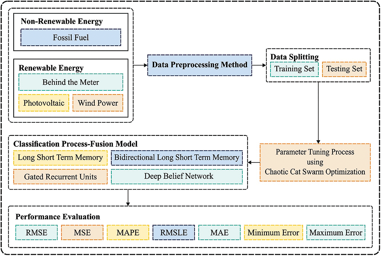
Figure 1: Overall process of MDLFM-ECP model

3.1 Stage 1: Data Pre-Processing

In the RE and NRE sources, missing data exist due to climate, preservation, abandoned winds, sensors fault, measurement error, etc. The new information from predicting techniques adversely affects outcomes’ forecast accuracy and consistency. Therefore, the pre-treatment of historical information to wind power forecasts is attracting considerable attention. During this analysis, a 2-manner comparative technique was utilized for identifying the abnormal information because of the inability of manual work to find the wrong information from huge datasets. The 2-manner comparative technique enhances the condition in which the typical lateral comparative approach could not effectually manage the loss and mutation of continuous data from the procedure of judgment and modification of abnormal information. Also, this work accepts the succeeding formula for completing the linear transformation to 0 and 1 [10]:

x_i=xi−xminxmax−xmin(1)

where x_i implies the normalisation of new data, xmax and xmin signify the maximal and minimum of new data correspondingly.

3.2 Stage 2: Fusion-Based Prediction Process

At this stage, the pre-processed data are applied to the fusion model, which consists of four DL models. The fusion of features is an important process that integrates multiple features. It mainly depends upon the features fusion using entropy, and the four vectors can be represented using Eqs. (2)–(4):

fGRU1×n={GRU1×1,GRU1×2GRU1×3,⋯,GRU1×n}(2)

fLSTM×m={LSTM1×1,LSTM1×2,LSTM1×3,⋯,LSTM1×m}(3)

fBiLSTM×l={BiLSTM1×1,BiLSTM1×2,BiLSTM1×3,⋯,BiLSTM1×l}

fDBN1×p={DBN1×1,DBN1×2,DBN1×3,⋯,DBN1×p}(4)

Integrating derived features into a single vector [19] using Eq. (5).

Fused(featuresvector)1×q=∑i=14 {fGRU1×n,fLSTM×m,fBiLSTM×l,fDBN1×p(5)

where f is the fused vector (1×1186). The entropy is utilized on the feature vectors to choose the optimum ones using the score.

3.2.1 GRU Model

GRU is a simple variant of LSTM, which consists of 2 gates, an “update gate” that has an input gate, forget gate and a “reset gate”. The GRU has no other memory cell for keeping the data. Hence, it could only control data inside the unit [20].

updategate=sigmoid(WugXt+Wught−1)(6)

restgate=siynoid(WrgXt+Wrght−1)(7)

h~=tanh(W(restgate)t⊗+Wht−1,Xt)(8)

hτ=(1−(updaτegate)t)⊗ht−1+(updaτegate)τ⊗h~(9)

Now, updategate in Eq. (6) determine how much data/contents is upgraded. In Eq. (7), restgate is the same as updategate; when the gate is fixed to 0, it reads the input sequence and forgets the formerly estimated state [20]. Furthermore, h~t demonstrates a similar function as in recurrent unit and ht of GRU at t time denotes the linear interpolation amongst the present h~t and prior ht−1 activation state.

3.2.2 LSTM and BiLSTM Models

RNN has been used for regression problems with the consideration of temporal dependency. The unfolded RNN holds the capacity to operate present data through preliminary data. In the meantime, RNN suffers from the issue of training the long-term dependency, i.e., resolved by the variations of RNN. Therefore, the LSTM is proposed as an advanced RNN network and addresses the limitations of RNN using hidden layer units called memory cells. It is controlled by 3 gates such as output, forget, and input gates [21]. Fig. 2 depicts the architecture of the LSTM model.

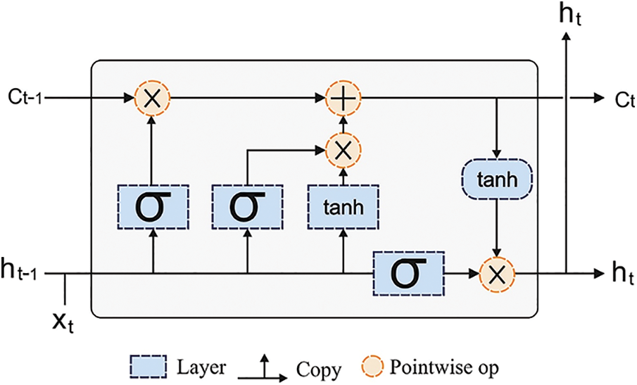
Figure 2: Structure of LSTM

The process of input, as well as output gates, is utilized for controlling the flow of memory cell input and output to the remaining networks. Additionally, forget gate was appended to the memory cell that passes the outcome data through higher weights before the following neurons. The data exist in memory based on the higher activation result; when the input unit holds higher activation, the data is saved in the memory cell. Furthermore, when the output element has higher activation later, it passes the data to the following neurons. Or else, input data with the highest weights reside in memory cells. LSTM model computes the map among output and input sequences, viz., X=(X1,X2,…,Xn) and =(y1,y2,…,yn). Calculate using the succeeding formula [21]:

forgetgate=sigmoid(WfgXt+Whfght−1+bfg)(10)

inputgate=sigmoid(WigXt+Whight−1+big)(11)

0utputgate=sigmoid(WogXt+Whoght−1+bog)(12)

(C)=(C)t−1⊗(forgetgate)t+(inputgate)t⊗(tanh(WCXt+WWhCht−1+bC))(13)

ht=outputgate⊗tanh((C)t−1)(14)

In Eqs. (9)–(13) Wig, Wog, WhC, Wfg and bfg, big, bog, bC represents the weight and bias parameter correspondingly of 3 gates as well as a memory cell. Now, ht−1 represents the previously hidden layer unit that element-wise added to the weight of 3 gates. Afterwards, the processing of Eq. (12), (C)t becomes the present memory cell unit. Eq. (13) demonstrates the element-wise multiplication of previously hidden unit output and prior memory cell unit. Add the non-linearity above the 3 gates through tanh and sigmoid activation functions that are demonstrated in Eqs. (9)–(13). Now, t−1 and t represent previous and present time steps.

To address the limitation of LSTM cell, i.e., capable of processing prior content but not utilising the upcoming one. It developed the BRNN method, i.e., contained 2 different LSTM hidden units with equivalent output in contradictory directions. This framework can employ prior and upcoming data in the output layer. The input series X=(X1,X2,…,Xn) in Bi-LSTM is evaluated in forwarding way as ht→=(h1→,h2→,hn→)and backward directions as ht←=(h1,h2,hn). The final out of this cell yt is created using ht→ and ht←, the last sequence of outlooks such as =(y1,y2,…yt…,yn). Fig. 3 illustrates the single-cell Bi-LSTM model.

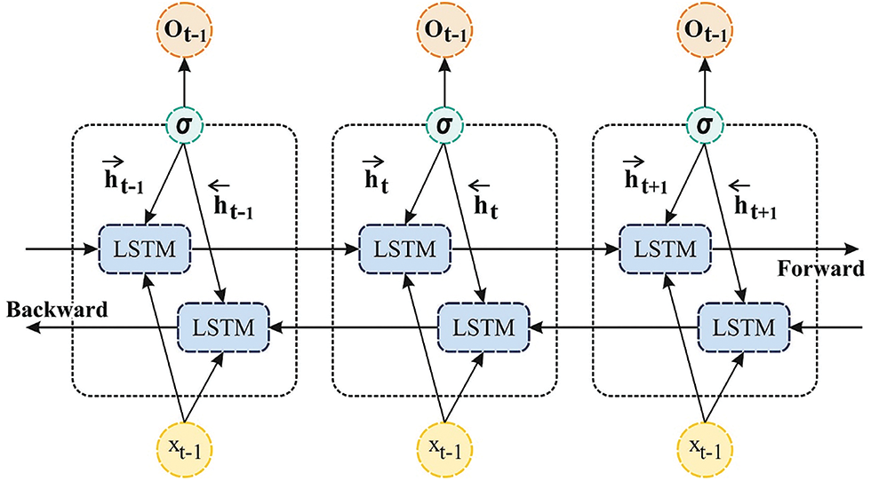
Figure 3: Framework of Bi-LSTM

3.2.3 DBN Model

DBN holds a bi-directional association known as RBM type connection on every peak layer while the underneath layer has only top/down association. They are trained layer-wise as pretraining. The pretraining exists by training the networking elements-wise bottom-up approach, viz., by processing the first 2 layers as an RBM, later preparing the 2nd and 3rd layers as another RBM, and eventually preparing for this parameter. Fig. 4 demonstrates the framework of the DBN model. The DBN model can be mathematically formulated by [22],

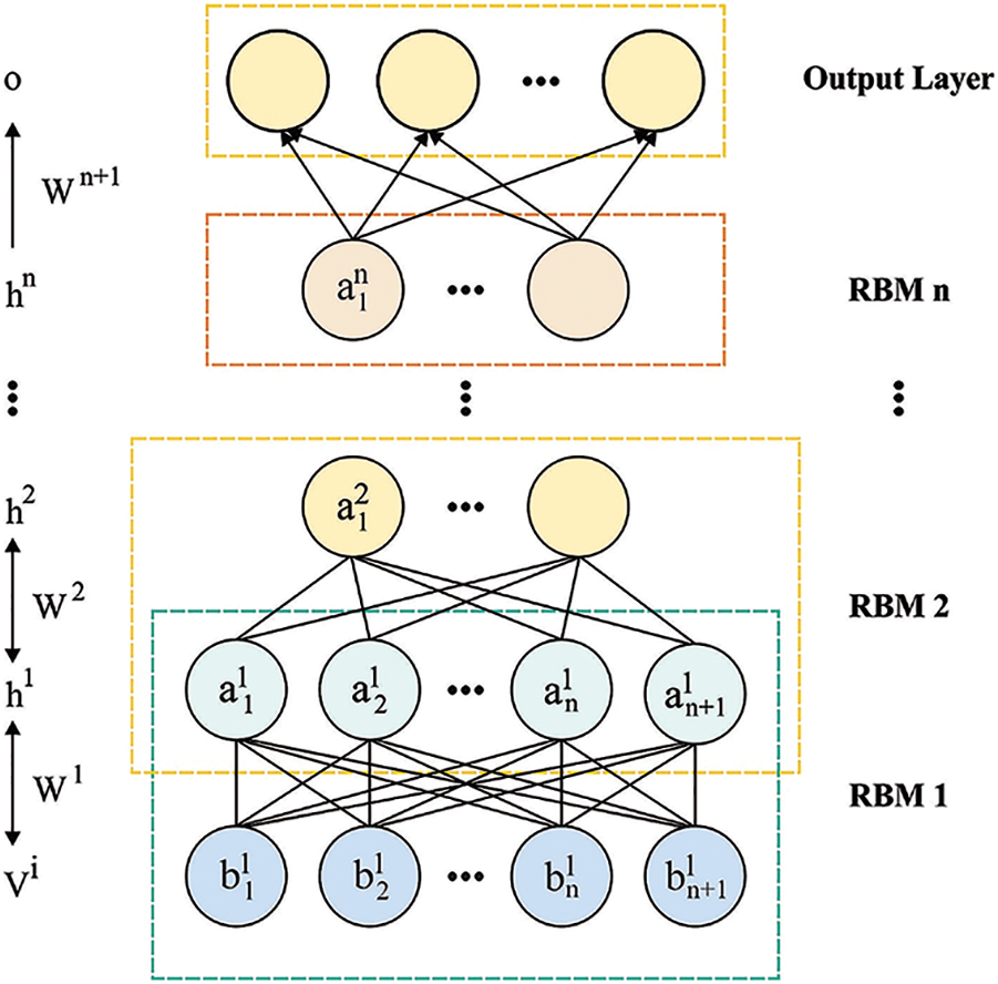
Figure 4: DBN structure

P(x,h1,…,h1)=(∏k=01−2P(hk|hk+1))P(h1−1,h1)(15)

whereas x=ho, P (hk|hk+1) represent a limited allocation for the observable unit habituated on the hidden unit of RBM at k-th level, and P (hl−1,h1) denotes the visible, hidden combined allocation in the top-level RBM [22]. DBN method for the combined allocation among hidden layers hk and the observed vector x. A graphic depiction of the DBN is demonstrated in Fig. 4.

3.3 Stage 3: Hyperparameter Tuning Using CCSO Algorithm

The CCSO is a population-based metaheuristic approach stimulated by the natural characteristics of cats and consists of two sub-models: tracing mode (TM) and seeking mode (SM), that defines the nature of the cats. This technique presented the optimization problem in the continuous field, as defined below.

f(x)(16)

where x∈RN, and M={x∈RN|li≤xi≤ui,i=1,2,⋯,N}⊆RN, with li and ui present the lower as well as upper bounds of xi correspondingly. The structure of the CCSO technique is explained in the subsequent 6 steps:

Step 1: Generate N cat from the procedure.

Step 2: Arbitrarily sprinkle the cat into the n-dimension solution space and arbitrarily choose values in the range of maximal velocity to the velocity of all the cats. Next, it randomly picks amount of cats by setting TM based on MR (mixture ratio) and another set as SM.

Step 3: Estimate the fitness value (FV) of all cats by implementing the places of cats into the fitness function (FF) that demonstrates the condition of our purpose and preserves the optimum cat as to memory. Noticeably, it can only require remembering the place of an optimum cat (xbest) because it signifies the optimum solution so far.

Step 4: Shift the cats based on the flags. When catk is in SM, implement the cat to the SM procedure or the trace mode procedure. These procedure steps are projected above.

Step 5: Re-pick the number of cats by setting a trace mode based on MR; afterwards, set another cat as SM.

Step 6: Verify the end criteria. If fulfilled, end the process; else, reiterate steps 3–5. The chaotic map has been discrete-time dynamical model

xk+1=f(xk),0<xk<1,k=0,1,2,⋯(17)

The chosen chaotic map takes chaotic numbers from 0 and 1. It offers novel techniques presenting a chaotic map in CCSO to improve global convergence by absconding the local solution.

Examining cat behaviors, the 2 behaviors of cats, such as TM and SM: Cats often remain attentive and move very slowly. This behavior of the cat is denoted as SM. Once the existence of prey is recognized, the cat chases it rapidly. This behavior of a cat, viz., chasing with higher speed, is denoted as TM. The cat’s location is utilised to represent the solution set [23]. All the cats have velocity and position for every fitness value and dimension. Besides this, a flag is utilized to identify the cat in TM/SM.

In TM, the solution search (Update the location of catk) of CCSO is determined as Eq. (18):

xk,i=xk,i+vk,i+r1×c1×(xbesti−xk,i)i=1,2,⋯,N(18)

Whereas xbest,i represent the cat’s location with optimal FV; xk,i indicates the location of catk. c1 signifies a constant, and r1 denotes an arbitrary number in zero and one [0, 1].

Based on Eq. (18), the arbitrary number r1 can be altered by the elected chaotic map, and the assimilation is altered as

xk,i=xk,i+vk,i+r1×{cs}×(xbest,i−xk,i),i=1,2,⋯,N(19)

whereas {cs} denotes a chaotic sequence depending on the elected map.

4  Performance Validation

This section investigates a comprehensive experimental validation of the MDLFM-ECP technique on the test data, and the results are examined under varying aspects. In this work, four kinds of energy sources in dataset namely fossil fuel (FF), behind the meter (BTM), wind power (WP), and power purchase agreement (PPA). Table 1 provides a detailed comparative results analysis of the MDLFM-ECP technique [24]. The proposed model is simulated using Python 3.6.5 tool on PC i5-8600k, GeForce 1050Ti 4GB, 16GB RAM, 250GB SSD, and 1TB HDD. The parameter settings are given as follows: learning rate: 0.01, dropout: 0.5, batch size: 5, epoch count: 50, and activation: ReLU.

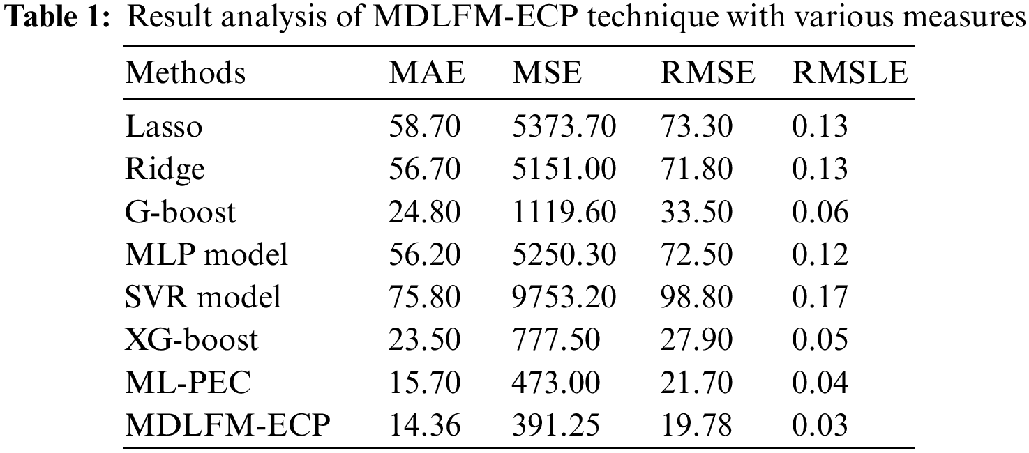
Fig. 5 offers the MAE and RMSE results of the MDLFM-ECP and existing techniques. Observing the results in terms of MAE, the results portrayed that the SVR, Lasso, Ridge, and MLP techniques have accomplished poor outcomes with higher MAE values of 75.8, 58.7, 56.7, and 56.2, respectively. In addition, the G-Boost and XGBoost techniques have resulted in moderately closer MAE of 24.8 and 23.5, respectively. Though the ML-PEC technique has gained near optimal MAE of 15.7, the proposed MDLFM-ECP technique has showcased effective outcomes with the least MAE of 14.36. Likewise, on detecting the outcomes for RMSE, the results exhibited that the SVR, Lasso, Ridge, and MLP approaches have accomplished the least result with the maximal RMSE values of 98.8, 73.3, 71.8, and 72.5, correspondingly. Moreover, the G-Boost and XGBoost systems have correspondingly resulted in moderately closer RMSE of 33.5 and 27.9. But, the ML-PEC manner has attained near optimum RMSE of 21.7, and the projected MDLFM-ECP technique has outperformed the effective outcome with the minimum RMSE of 19.78.

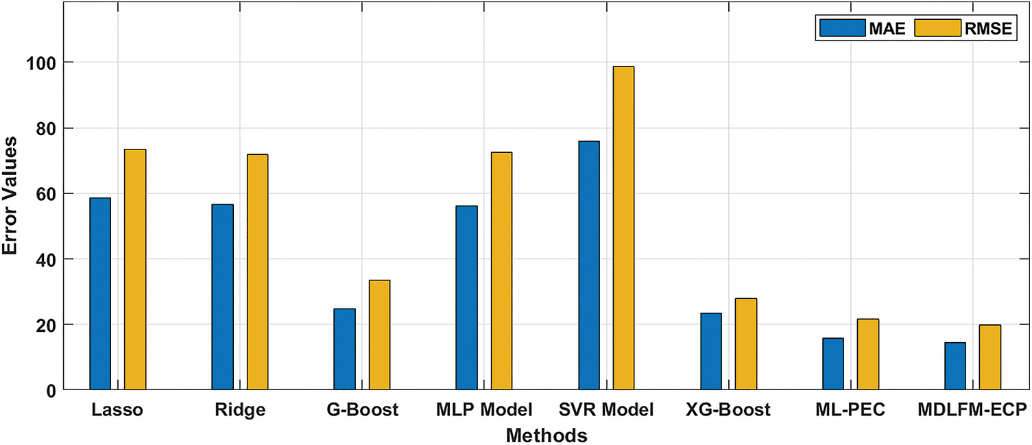
Figure 5: Result analysis of MDLFM-ECP technique in terms of MAE and RMSE

Fig. 6 provides the MSE analysis of the MDLFM-ECP manner with existing techniques. The figure shows that the SVR, Lasso, Ridge, and MLP systems have accomplished poor outcomes with higher MSE values of 9753.2, 5373.7, 5151.0, and 5250.3, respectively. In addition, the G-Boost and XGBoost approaches have resulted in moderately closer MSE of 1119.6 and 777.5, respectively. Though the ML-PEC scheme has gained near optimal MSE of 473.0, the presented MDLFM-ECP technique has outperformed effective outcomes with the least MSE of 391.25.

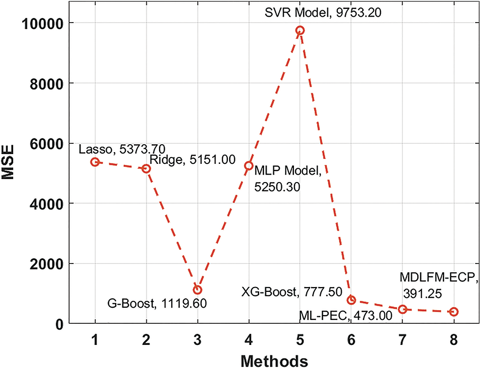
Figure 6: MSE analysis of MDLFM-ECP model with existing approaches

Fig. 7 gives the RMSLE results of the MDLFM-ECP and existing approaches. The results demonstrated that the SVR, Lasso, Ridge, and MLP techniques had accomplished poor outcomes with superior RMSLE values of 0.17, 0.13, 0.13, and 0.12. Followed by the G-Boost and XGBoost manners have resulted in moderately closer RMSLE of 0.06 and 0.05, respectively. Afterwards, the ML-PEC technique gained near optimal RMSLE of 0.04, and the presented MDLFM-ECP technique has portrayed a productive outcome with a minimal RMSLE of 0.03.

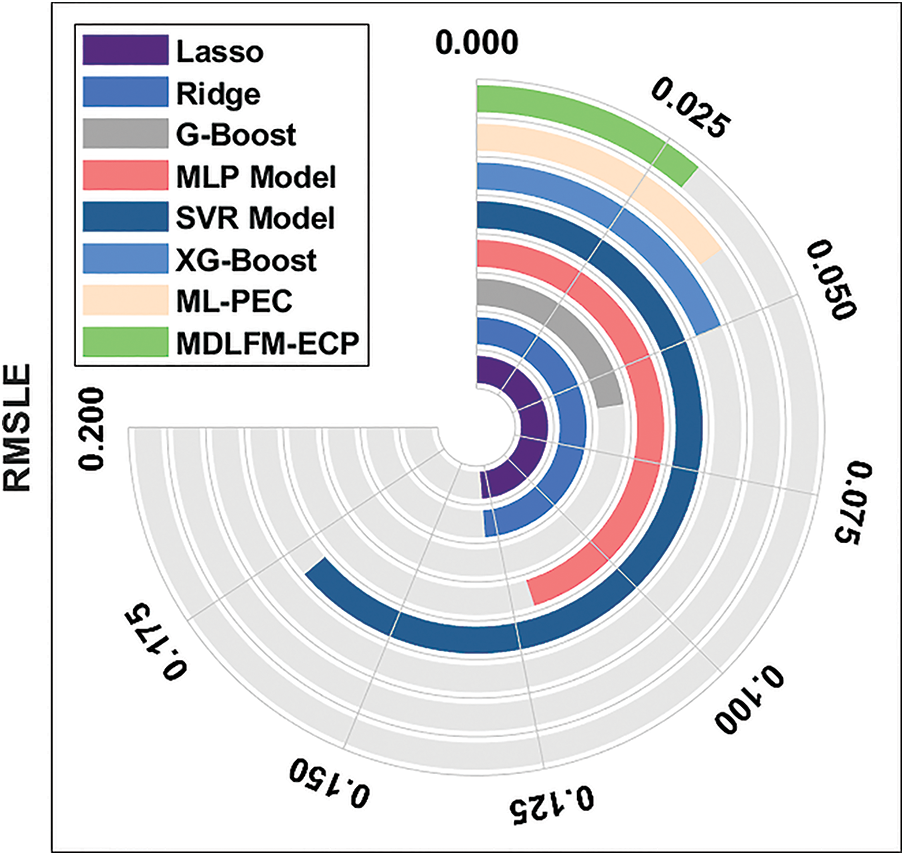
Figure 7: RMSE analysis of MDLFM-ECP model with existing manners

Table 2 provides the results analysis of the proposed model in terms of actual and predicted error under three runs. Fig. 8 demonstrates the results analysis of the MDLFM-ECP technique in terms of actual vs. predicted error under run-1. The results demonstrated that the proposed model had attained the least differences between the actual and predicted error.

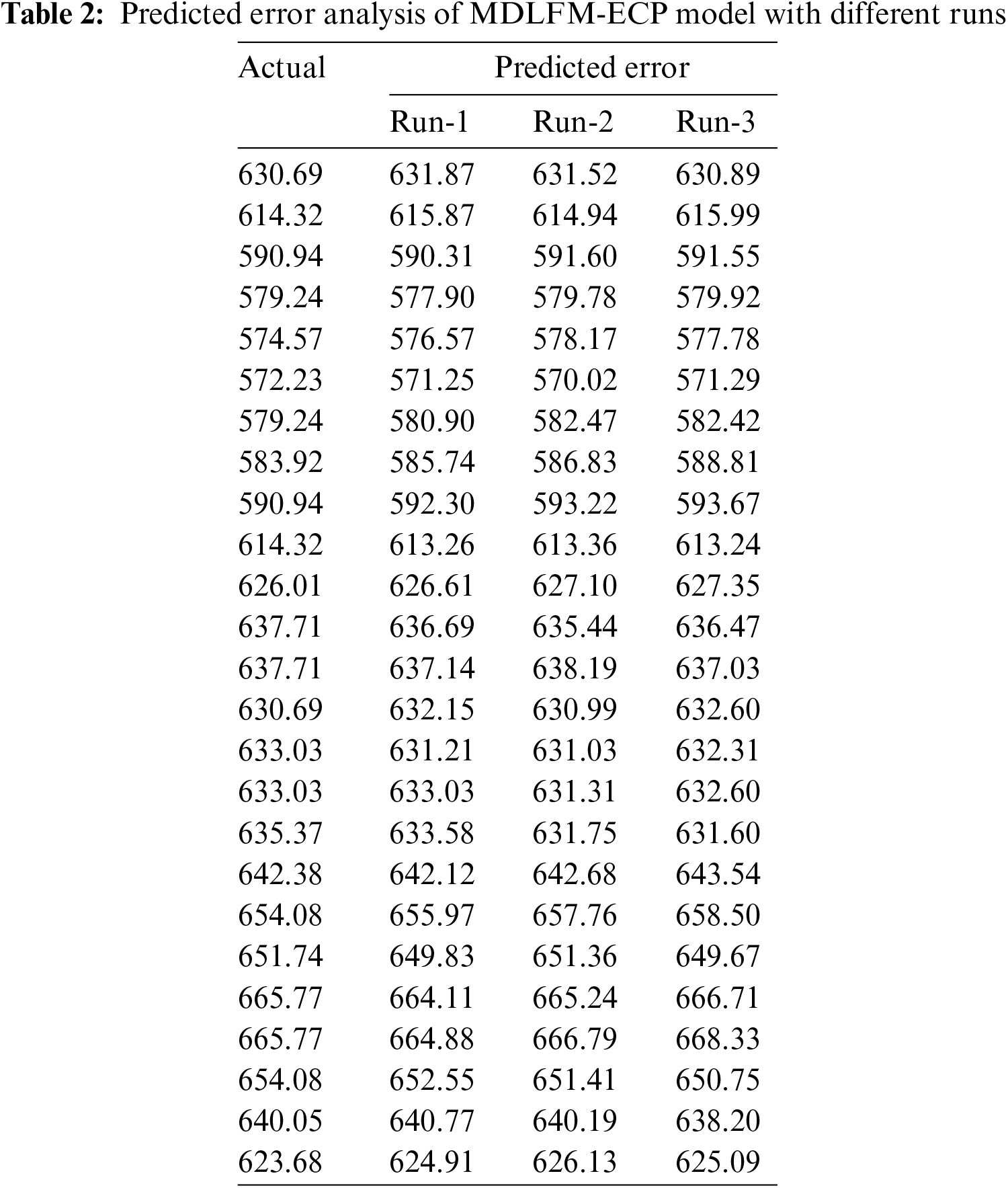
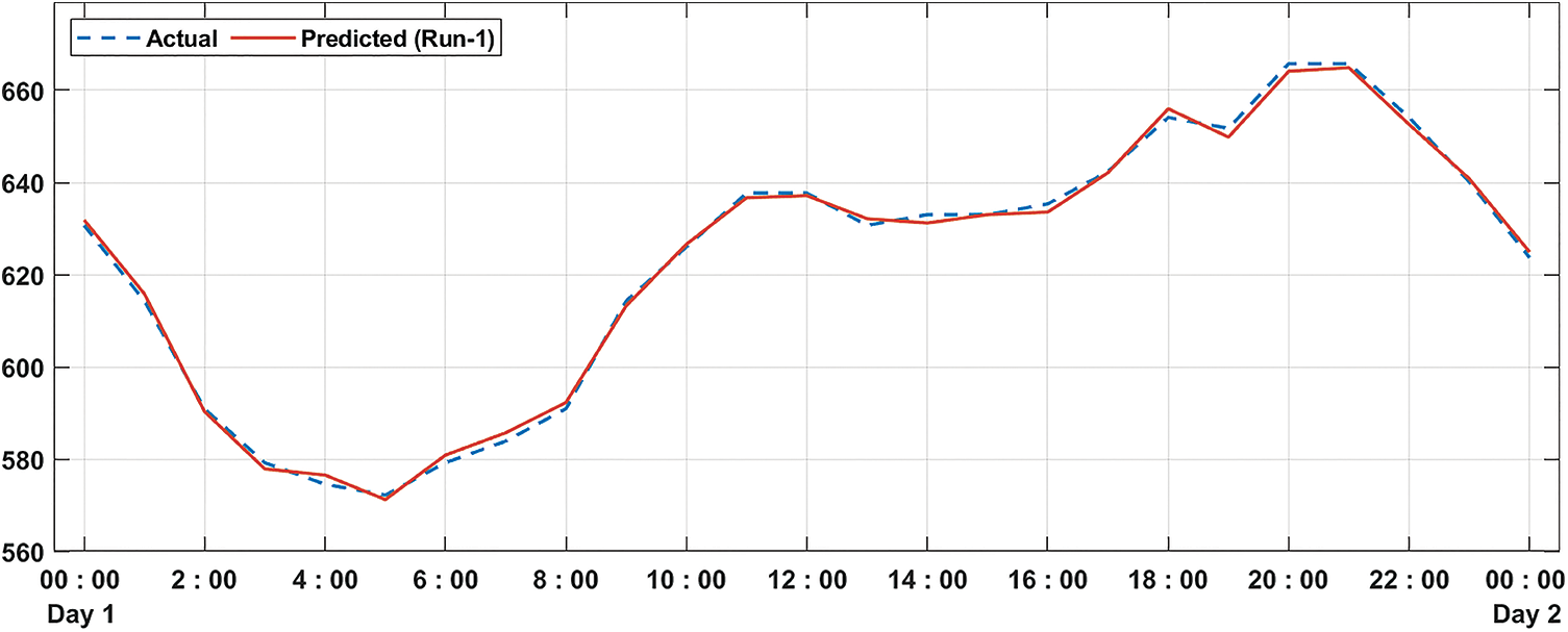
Figure 8: Predicted error analysis of MDLFM-ECP model on run-1

Fig. 9 showcases the performance analysis of the projected method in terms of actual vs. predicted error under run-2. The outcomes showed that the presented system had attained minimum differences between actual and predicted errors.

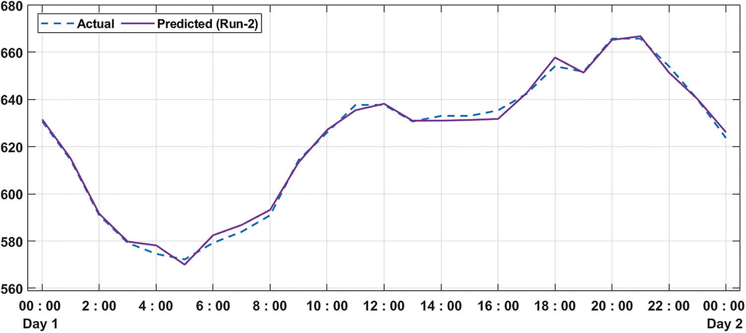
Figure 9: Predicted error analysis of MDLFM-ECP model on run-2

Fig. 10 illustrates the performance analysis of the proposed approach with respect to actual vs. predicted error under run-3. The results outperformed that the projected model has gained minimum differences between the actual and predicted error.

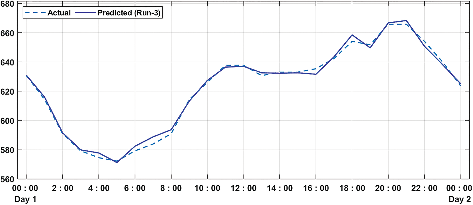
Figure 10: Predicted error analysis of MDLFM-ECP model on run-3

Finally, an overall MAPE analysis of the MDLFM-ECP technique with existing techniques takes place in Table 3 and Fig. 11. The experimental outcome has shown that the SVR, MLPRegressor, Ridge, and Lasso techniques have obtained higher MAPE of 21.61, 19.52, 10.41, and 10.39 respectively. In line with this, the XGBoost, Gradient Boosting, and ML-PEC-RE + NRE techniques have obtained moderately closer MAPE of 5.77, 6.86, and 4.29, respectively. However, the presented MDLFM-DCP technique has outperformed the other techniques with a MAPE of 3.58.

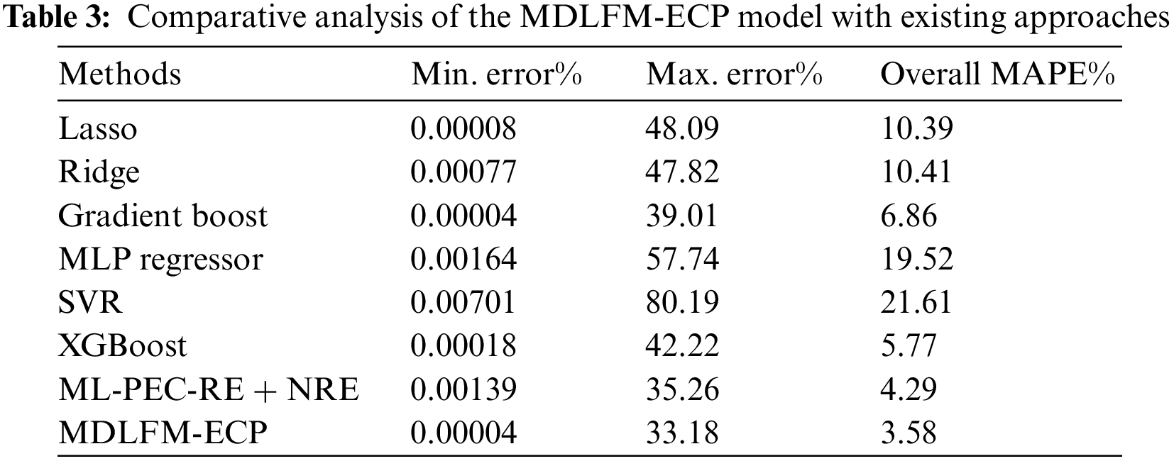
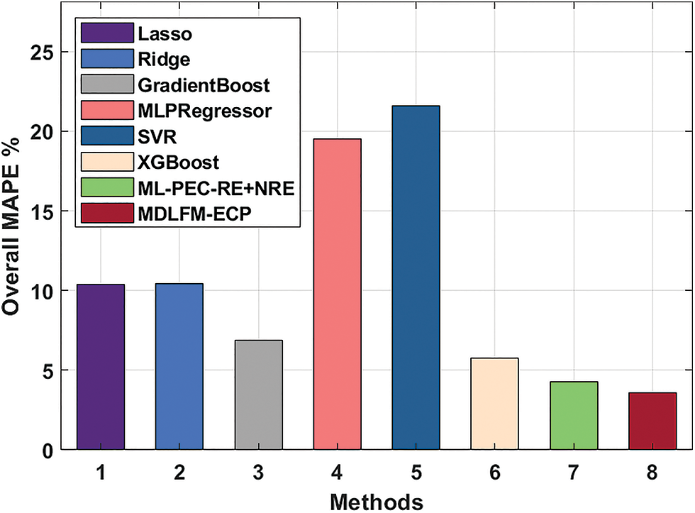
Figure 11: Comparative analysis of MDLFM-ECP model concerning overall MAPE

The results mentioned above ensure that the MDLFM-ECP technique has accomplished proficient outcomes with the minimum MAE, MSE, RMSE, RMSLE, and MAPE of 14.36, 391.25, 19.78, 0.03, and 3.58, respectively. Therefore, the proposed MDLFM-ECP technique is an effective tool for predicting energy utilization.

5  Conclusion

This study presents a new MDLFM-ECP technique for predicting energy utilization on RE and NRE sources. Actual data may influence the prediction performance of the results in prediction approaches. The proposed MDLFM-ECP technique involves pre-processing, DL based fusion model for prediction, and CCSO-based hyperparameter optimization. Moreover, the CCSO algorithm is applied to tune the hyperparameters of the DL algorithms. A series of simulations take place to ensure the superior efficiency of the MDLFM-ECP technique, and the simulation outcome emphasizes the improved results of the MDLFM-ECP technique over the other approaches. As a part of the future scope, the presented MDLFM-ECP technique can be tested using real-time data.

Funding Statement: The authors extend their appreciation to the Deanship of Scientific Research at King Khalid University for funding this work through the Large Groups Project under grant number (71/43). Princess Nourah bint Abdulrahman University Researchers Supporting Project number (PNURSP2023R203), Princess Nourah bint Abdulrahman University, Riyadh, Saudi Arabia. The authors would like to thank the Deanship of Scientific Research at Umm Al-Qura University for supporting this work by Grant Code: 22UQU4340237DSR61. This study is supported via funding from Prince Sattam bin Abdulaziz University project number (PSAU/2023/R/1444).

Conflicts of Interest: The authors declare that they have no conflicts of interest to report regarding the present study.

References

1. T. Güney, “Renewable energy, non-renewable energy and sustainable development,” International Journal of Sustainable Development & World Ecology, vol. 26, no. 5, pp. 389–397, 2019. [Google Scholar]

2. I. Ozturk and A. Acaravci, “Electricity consumption and real GDP causality nexus: Evidence from ARDL bounds testing approach for 11 MENA countries,” Applied Energy, vol. 8, no. 8, pp. 2885–2892, 2021. [Google Scholar]

3. M. B. Jebli, S. B. Youssef and I. Ozturk, “Testing environmental Kuznets curve hypothesis: The role of renewable and non-renewable energy consumption and trade in OECD countries,” Ecological Indicators, vol. 60, pp. 824–831, 2011. [Google Scholar]

4. N. Apergis and D. C. Danuletiu, “Renewable energy and economic growth: Evidence from the sign of panel long-run causality,” International Journal of Energy Economics and Policy, vol. 4, no. 4, pp. 578–587, 2014. [Google Scholar]

5. A. E. Abouelregal and M. Marin, “The response of nanobeams with temperature-dependent properties using state-space method via modified couple stress theory,” Symmetry, vol. 12, no. 8, pp. 1276, 2020. [Google Scholar]

6. L. Malka, A. Daci, A. Kuriqi, P. Bartocci and E. Rrapaj, “Energy storage benefits assessment using multiple-choice criteria: The case of drini river cascade,” Albania Energies, vol. 15, no. 11, pp. 4032, 2022. [Google Scholar]

7. N. Suwal, X. Huang, A. Kuriqi, Y. Chen, K. P. Pandey et al., “Optimisation of cascade reservoir operation considering environmental flows for different environmental management classes,” Renewable Energy, vol. 158, no. 4, pp. 453–464, 2020. [Google Scholar]

8. M. Pérez-Ortiz, S. Jiménez-Fernández, P. A. Gutiérrez, E. Alexandre, C. Hervás-Martínez et al., “A review of classification problem, algorithms in renewable energy applications,” Energies, vol. 9, no. 8, pp. 607, 2016. [Google Scholar]

9. M. L. Scutaru, S. Vlase, M. Marin and A. Modrea, “New analytical method based on dynamic response of planar mechanical elastic systems,” Bound Value Probability, vol. 2020, no. 1, pp. 104, 2020. [Google Scholar]

10. L. Munkhdalai, T. Munkhdalai, K. H. Park, H. G. Lee, M. Li et al., “Mixture of activation functions with extended min-max normalization for forex market prediction,” IEEE Access, vol. 7, pp. 183680–183691, 2019. [Google Scholar]

11. A. Moradmand, M. Dorostian and B. Shafai, “Energy scheduling for residential distributed energy resources with uncertainties using model-based predictive control,” International Journal of Electrical Power & Energy Systems, vol. 132, no. 4, pp. 107074, 2021. [Google Scholar]

12. S. A. Nabavi, A. Aslani, M. A. Zaidan, M. Zandi, S. Mohammadi et al., “Machine learning modeling for energy consumption of residential and commercial sectors,” Energies, vol. 13, no. 19, pp. 5171, 2020. [Google Scholar]

13. Y. Liu, L. He and J. Shen, “Optimization-based provincial hybrid renewable and non-renewable energy planning-A case study of Shanxi, China,” Energy, vol. 128, no. 6095, pp. 839–856, 2017. [Google Scholar]

14. E. Elahi, C. Weijun, S. K. Jha and H. Zhang, “Estimation of realistic renewable and non-renewable energy use targets for livestock production systems utilising an artificial neural network method: A step towards livestock sustainability,” Energy, vol. 183, no. 1, pp. 191–204, 2019. [Google Scholar]

15. J. Behera and A. K. Mishra, “Renewable and non-renewable energy consumption and economic growth in G7 countries: Evidence from panel autoregressive distributed lag (P-ARDL) model,” International Economics and Economic Policy, vol. 17, no. 1, pp. 241–258, 2020. [Google Scholar]

16. M. Ikram, “Models for predicting non-renewable energy competing with renewable source for sustainable energy development: Case of asia and oceania region,” Global Journal of Flexible Systems Management, vol. 22, no. 2, pp. 133–160, 2021. [Google Scholar]

17. H. Zhao and W. Lifeng, “Forecasting the non-renewable energy consumption by an adjacent accumulation grey model,” Journal of Cleaner Production, vol. 275, no. 7, pp. 124113, 2020. [Google Scholar]

18. R. Nadimi and K. Tokimatsu, “Analyzing of renewable and non-renewable energy consumption via bayesian inference,” Energy Procedia, vol. 142, pp. 2773–2778, 2017. [Google Scholar]

19. T. Saba, A. S. Mohamed, M. El-Affendi, J. Amin, M. Sharif et al., “Brain tumor detection using fusion of hand crafted and deep learning features,” Cognitive Systems Research, vol. 59, no. 1, pp. 221–230, 2020. [Google Scholar]

20. R. Dey and F. M. Salem, “Gate-variants of gated recurrent unit (GRU) neural networks,” in IEEE 60th Int. Midwest Symp. on Circuits and Systems (MWSCAS), Boston, MA, USA, pp. 1597–1600, 2017. [Google Scholar]

21. F. Shahid, A. Zameer and M. Muneeb, “Predictions for COVID-19 with deep learning models of LSTM, GRU and Bi-LSTM,” Chaos Solitons & Fractals, vol. 140, no. 14, pp. 110212, 2020. [Google Scholar]

22. K. Mathivanan, D. Thirumalaikumarasamy, M. Ashokkumar, S. Deepak and M. Mathanbabu, “Optimization and prediction of az91d stellite-6 coated magnesium alloy using box behnken design and hybrid deep belief network,” Journal of Materials Research and Technology, vol. 15, no. 1, pp. 2953–2969, 2021. [Google Scholar]

23. D. Gabi, N. M. Dankolo, A. S. Ismail, A. Zainal, Z. Zakaria et al., “Non-preemptive chaotic cat swarm optimization scheme for task scheduling on cloud computing environment,” International Journal of Advanced Computer Research, vol. 9, no. 43, pp. 186–196, 2019. [Google Scholar]

24. P. W. Khan, Y. C. Byun, S. J. Lee, D. H. Kang, J. Y. Kang et al., “Machine learning-based approach to predict energy consumption of renewable and non-renewable power sources,” Energies, vol. 13, no. 18, pp. 4870, 2020. [Google Scholar]