Radon CLF: A Novel Approach for Skew Detection Using Radon Transform

1  Introduction

Numerous printed and handwritten documents have been converted to digital format in the digital age utilizing a variety of devices, including mobile phones and dedicated scanners. Unfortunately, this procedure is far from ideal, and the entire document image may suffer from degradations including skew distortion, motion blur, and noise. The accuracy and efficiency of document image segmentation and analysis in Optical Character Recognition (OCR) systems can be directly impacted by these affecting factors. Fig. 1 depicts the operational procedures of an OCR system ([1]). In all OCR systems, the preprocessing steps are fundamental tasks that can affect the system’s performance directly [2–7]. The following is a list of some of the most fundamental and significant preprocessing methods used in Document Image Analysis (DIA):

•   Binarization

•   Skew Detection

•   Skew Correction

•   Noise Removal

•   Image Quality Enhancement

•   Dual-page Splitting

•   Straighten Curved Text Lines

•   Baseline Detection & Extraction

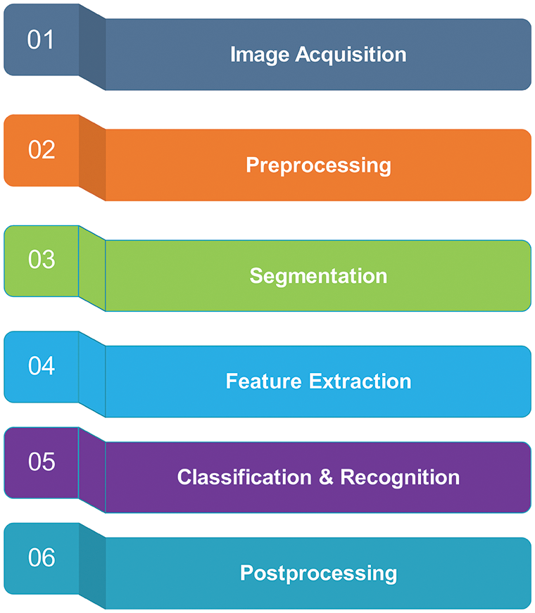
Figure 1: The different steps of any optical character recognition (OCR) system [1]

In general, skew detection is a primary step that plays a critical role in obtaining a high accuracy DIA system. The skewness in a document image can degrade exceedingly subsequent document processing algorithms in an OCR system.

In this work, the skew issue in input document images is the main focus. In this regard, a new dataset named DSI5000 (5000 Directional Synthetic Images) was created and developed by us. It includes about 5696 Directional Synthetic Images (DSI) with different intensities, angles, and frequencies to analyze the accuracy of the proposed Radon Transform Curve Length Fitness Function (CLF) algorithm so-called the Radon CLF. The Radon CLF model tries to benefit Radon space characteristics. Based on an innovative fitness function definition for a projected signal of the Radon space, the Radon CLF explores the dominant angle more efficiently for a 1D signal rather than the 2D input image. In this study, we have concentrated on the speed, robustness (against the noise effect), and the accuracy of the proposed model for the skew detection problem.

The many sections of this paper are arranged as follows: Section 2 introduces and discusses related works. Section 3 describes the proposed approach for skew detection. Experimental results and comparative analysis are the subject matter of Section 4. Finally, Section 5 includes the conclusion and future studies.

2  Related Works

Many approaches based on projection profile, topline, and scanline methods, have been used in the past to conduct skew detection on images. These are the most straightforward and often used approaches to identify document skew; however, the majority of them involve slow algorithms with low accuracy. These techniques generally rely on the fonts and grammatical structure of a given language as well. They do not perform well enough with manuscripts that either incorporate multiple languages or different fonts, in practice. For example, an approach using the horizontal projection histogram for just Arabic text was presented by [8]. They present a method that was based entirely on polygonal approximated skeleton processing.

In Signal & Image Processing and Computer Vision theory, there are many utilitarian directional filters and transforms, for example: the Hough Transform (HT), the Gabor Wavelet Transform (GWT), and Directional Median Filters (DMF). These directional filters can be used in the analysis of the directional patterns ([9–13]). For example, [14] used Hough Transform and Run-Length Encoding (RLE) algorithms for the skew detection problem. In 2010, an algorithm was proposed by [15]. It has three steps: firstly, the projection of the vertical and horizontal graphics of the image was eliminated. A binary image was applied to the dilation operation. In the last phase, the skew angle was achieved with the help of the Hough Transform. The proposed algorithm can detect the skew angle in the range between −90◦, and +90◦, with high precision.

Reference [16] deployed the Fast Hough Transform (FHT) to detect skew angles. In this approach, there is no need for a binary representation of the text image. The Fast Hough Transform was applied on both vertical and horizontal lines. This technique reduced the computational cost; while, the calculated error was around 0.547. Skew detection approaches found on Hough Transform usually impose a high computational cost. Reference [17] improved an algorithm based on least squares to handle a multi-skew problem. In [18] and [19], they used a binary text document dataset to evaluate the skew angle with the help of linear regression algorithms. The time cost of these methods was smaller than other algorithms based on the Hough Transform. The algorithm performed text lines classification. To increase the accuracy, the variation of skew angle was calculated in the ±10◦ range. With increasing the angle, the accuracy was reducing to the same ratio.

In [20], they introduced a method that inscribes the text in a document image found on an arbitrary polygon and derivation of the baseline from the polygon’s centroid. It had proven that their algorithm was suitable to apply to documents written in different fonts. In [21], an algorithm was presented to perform skew angle correction for handwritten text documents. The algorithm used the Hough Transform and the restricted box technique. In this algorithm, linear regression functions have been used to compute the skew angle in a manuscript. The algorithm’s main point is that it displays parallel rectangles in the binary image with the lowest number of pixels in line with horizontal and vertical orientations. Then, the linear regression function would be calculated for the skew angle. In [22], morphological functions were used to detect skew angles. These functions can be analyzed in the frequency domain found on Fourier Transform (FT). The Fourier Transform could detect text distortion in different languages, including English, Hindi, and Punjabi. In [23], a nearest-neighbor-chain or NNC algorithm was introduced with language-independent capability. Size restriction was the main challenge to the detection of nearest-neighbors (NN), before the skew detection.

In [24], the Principle Component Analysis (PCA) and its wide applications in Image & Signal Processing, were presented. In [6], finding the skew angle has done using the PCA approach. After converting the input document into a binary picture, the algorithm utilized Sobel and Gaussian filters. It helps to find edges and reduce noise. The PCA-based method gets the covariance matrix, after which it produces the Eigen values and Eigen vectors, and then calculates the unit vector for the principal component. Later, the document’s skew angle can be determined using the principal components. The introduced algorithm could get an accuracy of about 90% but with a high time cost.

In [25], they presented an adaptive Skew Correction technique for document images. It uses image’s layout features and classification to detect the type of document image. Three different classes, named Text image, Form image, and Complex image, were considered in the classification problem. Then, based on the type of document image, one of three proposed algorithms: Morphological Clustering (MC), Piecewise Projection Profile (PPP), and Skeleton Line Detection (SKLD), should be used to correct the skew of a document image.

Transferring the input image to Radon space and using a strong feature extraction method like the suggested Radon CLF, is an appropriate alternative to working with highly loaded 2D data. It can benefit high-speed processing algorithms in a one-dimensional signal space rather than image space. Radon CLF can also lead to improved results in terms of computational time and accuracy. The subsequent sections will go through this idea.

3  Methodology

Today, enormous amounts of information are stored in printed documents. The primary and important step in the processing of paper-based documents is to convert them into digital records. In practice, the main problem is that the document may be rotated unaptly on a flatbed scanner at a random angle. In this situation, the scanned image may be skewed. The skew is considered a surplus distortion which can degrade the image quality. The skew can impose severe challenges in digital image analysis and deteriorate the overall performance of any OCR system. In this section, the methodology and our proposed approach to detect skew is discussed in more detail. In Fig. 2, a general scheme of our proposed approach is presented.

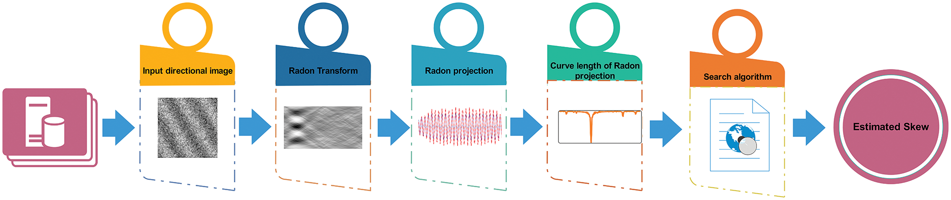
Figure 2: The proposed Radon CLF algorithm for skew detection in document images

3.1 The Radon Transformation

The Radon function is calculated from an image matrix such as f(x, y) in specific directions. The Radon function accounts for linear integrals over different paths or certain paths (from different sources/beams) in a specific direction [9,26–32]. This function takes multiple parallel-beam projections of the input image from different angles by rotating the source around the center of the image.

In Fig. 3, a single image at a specified rotation angle of the Radon transform is illustrated. Besides, Fig. 4 indicates the geometry of the Radon Transform.

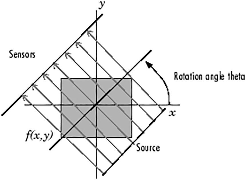
Figure 3: The parallel-beam projection at rotation angle [33]

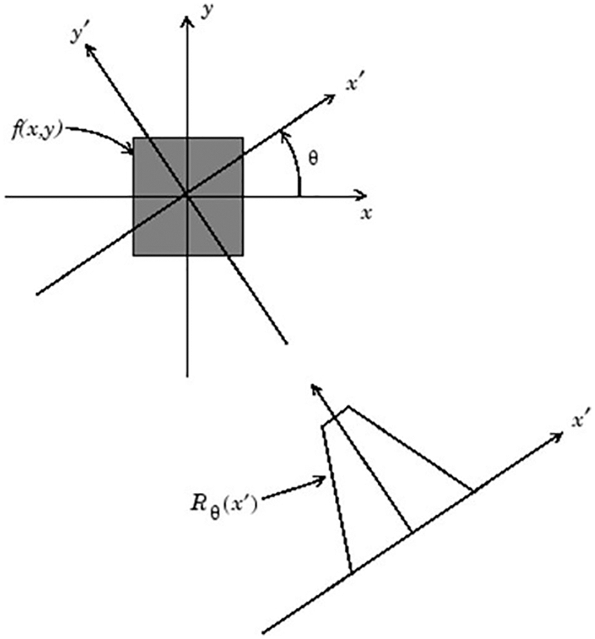
Figure 4: The Geometry of the Radon Transform [37]

The computation of projections can be down from any angle. Generally, the Radon transform (Rθ(x′)) of the function f(x, y) is the linear integral of it, in parallel to y’-axis [34–36] (see Eqs. (1) to (4)):

Rθ(x′)=∫−∞+∞f(ρ1x,y,θ,ρ2x,y,θ)dy(1)

ρ1x,y,θ=x′cos⁡(θ)−y′sin⁡(θ)(2)

ρ2x,y,θ=x′sin⁡(θ)+y′cos⁡(θ)(3)

[x′y′]=[cos⁡(θ)sin⁡(θ)−sin⁡(θ)cos⁡(θ)][xy](4)

where the pair (x’, y’) is the new place of the (x, y) after rotating with the angle theta in a two-dimensional Cartesian coordinate system.

3.2 Skew Detection

This section conceptualizes our new skew detection approach so-called Radon CLF (Radon Curve Length Fitness Function). Usually, the local region in a document image has a consistent orientation and frequency [38]. So, it can be modeled as a surface wave characterized entirely by the dominant orientation and frequency pattern. This approximation model is practical enough for our purpose of evaluating the performance of the Radon Transform for the skew estimation problem. According to Eq. (5), a local region of the image can be modeled as a surface wave [39]:

I(x, y)=Acos(2πf(x cos(θ)+y sin(θ)))(5)

where f is the frequency, the theta is the dominant orientation, and A is the amplitude of the cosine function. A is the intensity adjustment parameter of the synthesized image I(x, y). An example image and its projection by the Radon Transform are shown in Fig. 5. As it can be seen in the projection function in Fig. 5b, providing that it has been projected in the actual orientation, which is parallel to the local orientation of the input image, it can be approximately treated as a semi-sinusoidal plane wave. Besides, the noisy version of the image in Fig. 5a and its Radon projection are depicted in Fig. 6. Although, the noise power is utterly high (the Gaussian noise with the standard deviation (σ) about 20), the comparison between Figs. 5b, and 6b shows that the semi-sinusoidal structure of the Radon projection is still satisfied with a few distortions. Figs. 7 and 8 are depicted with a new angle. Now, two new Radon transform maps are compared between a noise-free directional image and its noisy version with σ = 9. With comparing two Figs. 7a and 8a in the image signal space, it can be viewed that the noise effect is quite eye-catching. On the other side, when we make comparison between Figs. 7b and 8b in the Radon space, it indicates that the presence of noise does not impact the projected pattern in this space, considerably.

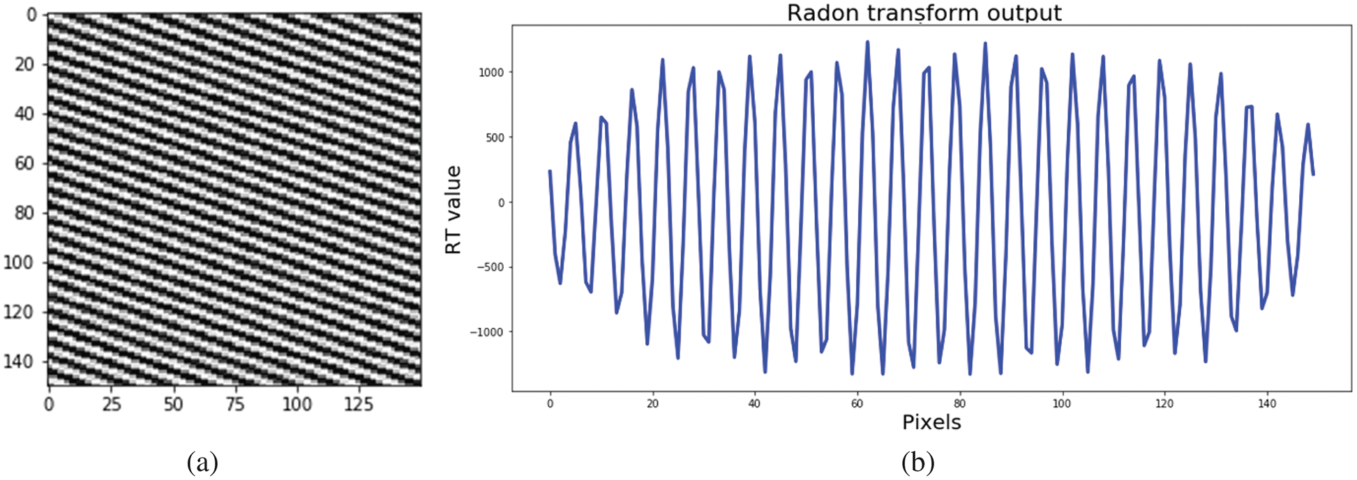
Figure 5: (a) A well-defined 150 × 150 synthetic image (x). (b) The Radon Transform: R(x)

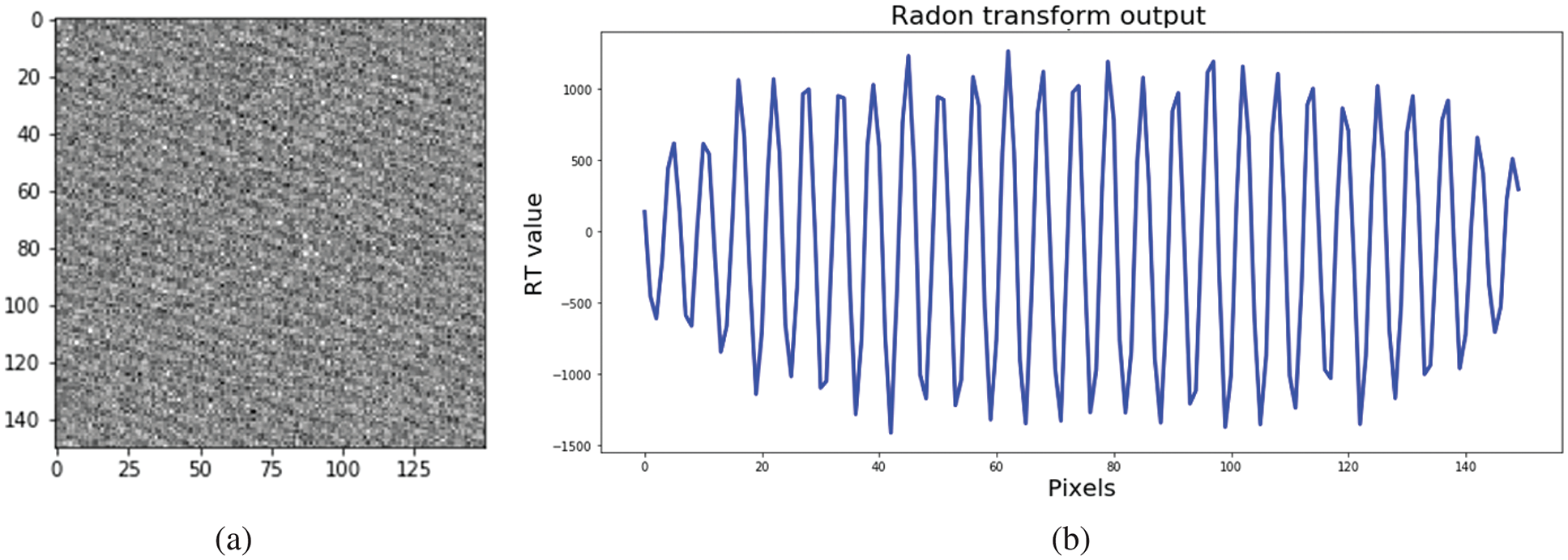
Figure 6: (a) A noisy synthetic image (Gaussian Noise with σ = 20). (b) The Radon Transform: R(x)

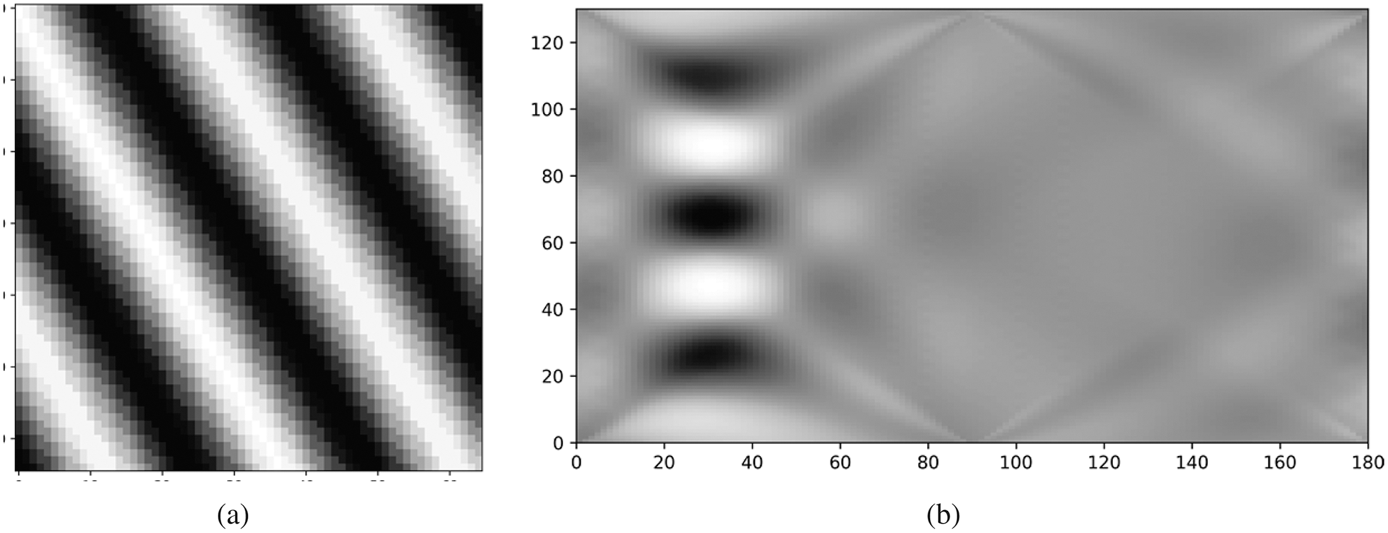
Figure 7: (a) A noise-free synthetic image with θ = 30 and σ = 0. (b) The Radon transform map of the image

Figure 8: (a) A noisy synthetic image with θ = 30 and σ = 9. (b) The Radon transform map of the image

These comparisons show that the proposed skew detection algorithm can abundantly tolerate the additive noise more efficiently in the Radon space rather than the signal space, providing that an appropriate feature extraction method is available for the Radon space. This observed phenomenon should be evaluated further in the following sections.

3.3 Curve Length of a Function

In Fig. 9, f(x) is shown as an example of an one-dimensional continuous function. The Arc length L of a function such as y = f(x) between a and b (from the point (a, f (a)) to the point (b, f (b))) can be derived using Eq. (6):

L=∫ab1+(dydx)2 dx(6)

where dydx denotes the first derivative of the function f(x). Supposing that C would be a curve in Euclidean (or, generally, a metric) space X = Rn, so C is a continuous function of an image where f: [a, b] → X of the interval [a, b] into X. From a partition a = x0 < … < xn−1 < xn = b of the interval [a, b], there is a finite collection of points f(x0), f(x1),…, f(xn−1), and f(xn), which can be used to calculate the length of the line segment connecting the two points. According to Eq. (7), the arc length L of C is then defined to be L(C):

L(C)=∑i=0n−1d(f(xi),f(xi+1))(7)

where the supermom is calculated of all possible sections of [a, b] and n is unbounded. This definition of the arc length does not require that C be defined by a differentiable function. Generally, the notion of differentiability is not defined in a metric space.

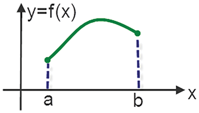
Figure 9: An example of 1D function f(x)

3.4 Definition of the Proposed Fitness Function

In the case of the discreet Radon function, Rθ(x), this article defines the curve length of the function, Lθ,Rθ, as Eq. (8):

Lθ,Rθ=∑xΔRθ(x)(8)

Thus, the estimated skew of an input image, θ^, can be obtained the using proposed Eq. (9):

θ^=Argmax(Lθ,Rθ)(9)

If the orientation is the same as the local skew, the projection function will result in a semi-sinusoidal plane wave. If not, the resultant pattern can be an erratic, non-sinusoidal signal with a smaller amplitude. This fact is shown in Fig. 10. Fig. 10 makes a comparison between Radon projection patterns on the actual orientation at θ = 70 (the red line with error = 0) and some incorrect orientations, such as 71 (error = + 1◦), and 60 (error = −10◦). This study proposes the curve length of the projected Radon pattern as a fitness function for skew estimation, and call it the Radon CLF algorithm.

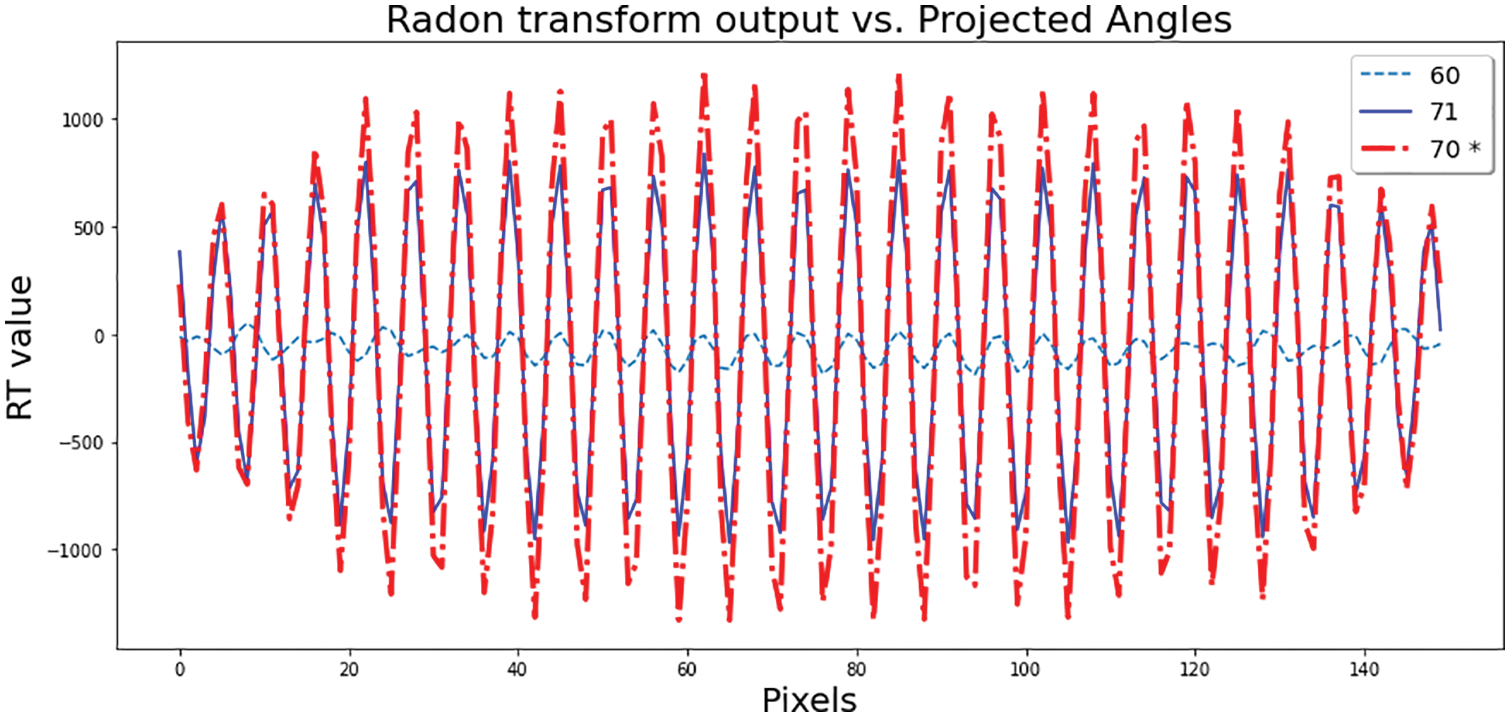
Figure 10: Comparison between Radon projection patterns on the actual orientation at θ = 70 (the red line with error = 0), and some incorrect ones such as 71 (error = + 1◦) & 60 (error = −10◦)

It will be shown that in the correct orientation, such as θ = 70 in Fig. 10, the length of the curve would be well over the curve lengths of other incorrect orientations.

3.5 Performance Evaluation Metrics

Performance metrics are a vital part of every algorithm analysis. To evaluate the performance of our proposed method, we have used the Mean Squared Error (MSE) (for both the skew estimator and image comparison), the Mean Absolute Error (MAE) (for the skew estimator), Accuracy (for the skew estimator), Peak Signal-to-Noise Ratio (PSNR) (for the images comparison), and Structural Similarity Measure (SSIM) (for the images comparison) along with the Computational Time.

In statistics, the MSE is considered the Mean Squared Deviation (MSD) of an estimator. It can measure the average of the square of the errors or the average squared difference between the actual/ground-truth value and the estimated value ([40]).

MSE=1n∑i=1n(θi−θ^i)2(10)

In Eq. (10), θi is the true value of the angle for the ith sample, and θ^i is the estimated angle for it. The θi−θ^i  is the error signal for the ith sample, and should be calculated for all n available samples.

In comparison to the MSE, the Mean Absolute Error or MAE is the absolute average of the difference between the ground-truth and the predicted value [40] (see Eq. (11)).

MAE=1n∑i=1n|θi−θ^i|(11)

In addition to MSE and MAE, the Accuracy is defined using Eqs. (12) to (14):

|T|=card(T) ↔ T={{∀Ii∈DB|θ−θ^=0}}(12)

where |T| is used for the cardinal of the set T, and it means the total number of error-free predictions (true predictions) in the whole dataset (Card (DB)). Similarly, the |F| is used for the cardinal of the set F which means the total number of false predictions (predictions with error) in the entire dataset.

|F|=card(F) ↔ F={{∀Ii∈DB|θ−θ^≠0}}(13)

Accuracy=|T||T|+|F|(14)

The 1D MSE formula can be extended to the 2D space ([41,42]): MSE2D. In this study, it is needed to compare two images as two matrices. Eq. (15) represents the MSE2D for two images:

MSE2D=1m×n∑i=0n−1∑j=0m−1(I(i,j)−I^(i,j)2(15)

where I(x, y) is an m×n original image while the I^(x,y) would be whether a noisy image or a disturbing version of the original image. The MSE2D measures differences between two images and shows the quality degradation. The zero MSE2D means that the two images are the identical (the perfect similarity).

The PSNR or Peak Signal-to-Noise Ratio also represents a measure of the image error. Both the PSNR, and MSE2D are usually used to measure an image’s quality after its variation ([41,42]). The PSNR can be calculated directly found on the MSE2D ([40]), according to Eq. (16):

PSNR=10×log10(2552MSE2D)(16)

In addition to PSNR and MSE2D, Structural Similarity Measure or SSIM have been deployed in this paper using Eq. (17) ([42]). In a 2D space, the MSE2D will calculate distance as the mean of the square error between each corresponding pixel for the two target images. In contrast, the SSIM tries to do the opposite, and looks for similarities within pixels ([42–44]). To remedy some of the issues associated with MSE for image processing, SSIM have used. In Eq. (17), μx and μy are the average of x and y while σ x and σ y are the standard deviation of them, respectively. Similarly, μx2 and μy2 denote the variances and σ xy is the covariance of x and y. The c1 and c2 are two adjustable constant parameters.

SSIM=(2μxμy+c1)(2σxy+c2)(μx2+μy2+c1)(σx2+σy2+c2)(17)

It is worth mentioning that the SSIM can vary between −1 and 1; where SSIM = 1 indicates the perfect similarity ([40,43,44]).

3.6 Skew Correction

When the skew angle is detected by an algorithm, the next step would be Skew Correction. Technically, it is just a simple rotation procedure for a 2D image. So far, different methods such as contour-oriented projection, direct/indirect based method, and others, have been introduced to correct skewed images. In our simulation, the rotation of an input image is done through the Affine Transformation (AT) using Eqs. (18) and (19) ([45]):

x∗=cos⁡(θ^)x+sin⁡(θ^)y(18)

y∗=−sin⁡(θ^)x+cos⁡(θ^)y(19)

Here, the (x, y) is the coordinates of a pixel in the skewed input image, θ^ denotes the detected angle, and (x*, y*) is a new place of the pixel.

4  Experimental Results

The introduced method was implemented in the Python programming environment using an Intel(R) Core(TM) i7-7700HQ 2.80 GHz CPU. To evaluate the model, a dataset called DSI5000 was created and developed by us. It has about 5696 Directional Synthetic Images (DSI) with different amplitudes (intensities), orientations (dominant directions), and frequencies (repetitive line patterns). In addition to DSI5000, many real-world scanned image documents were also included in our simulations. Both handwriting and printed samples were gathered at various resolutions from different Persian, Arabic, English, and multilingual resources.

In the first experiment, the Radon projections were calculated for an input image with an actual orientation of θ = 70. In Fig. 11, the Radon projections were illustrated for angles between 60 and 80 (including the true angle at θ = 70). It is a semi-sinusoidal pattern with well-defined harmonics and the highest amplitude for the projection angle = 70 (the correct orientation). θ0 refers to all other projection angles, such as 60, 65, 68, 69, 71, 72, 75, and 80. These angels have noticeably lower amplitudes. For θ0, it can be seen the more significant gap between a signal’s peaks compared to the peaks of the signal associated with the actual angle (θ). Then, Fig. 12 plots the Fitness Function vs. θ. It illustrates that the fitness function of a synthetic image with θ = 70 in the orientation ranges from 1 to 180 degrees has just one global minimum at θ = 70. Therefore, the skew of the image can be detected precisely and uniquely by the proposed fitness function. Our simulations indicate that the proposed feature extraction approach based on the curve length of the projected signal has the potential to discriminate these variations among projected signals, finely.

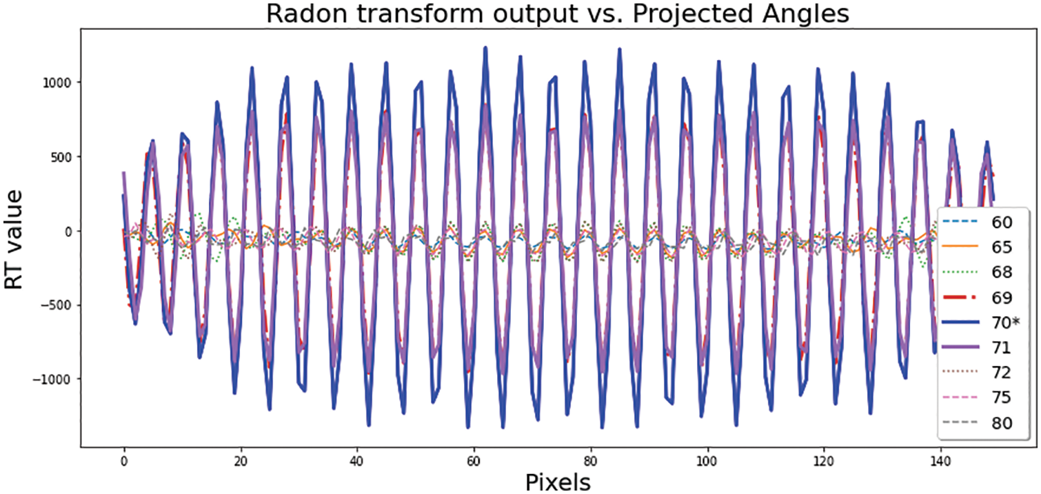
Figure 11: Radon Transform output for different projection angles (The correct orientation: θ = 70)

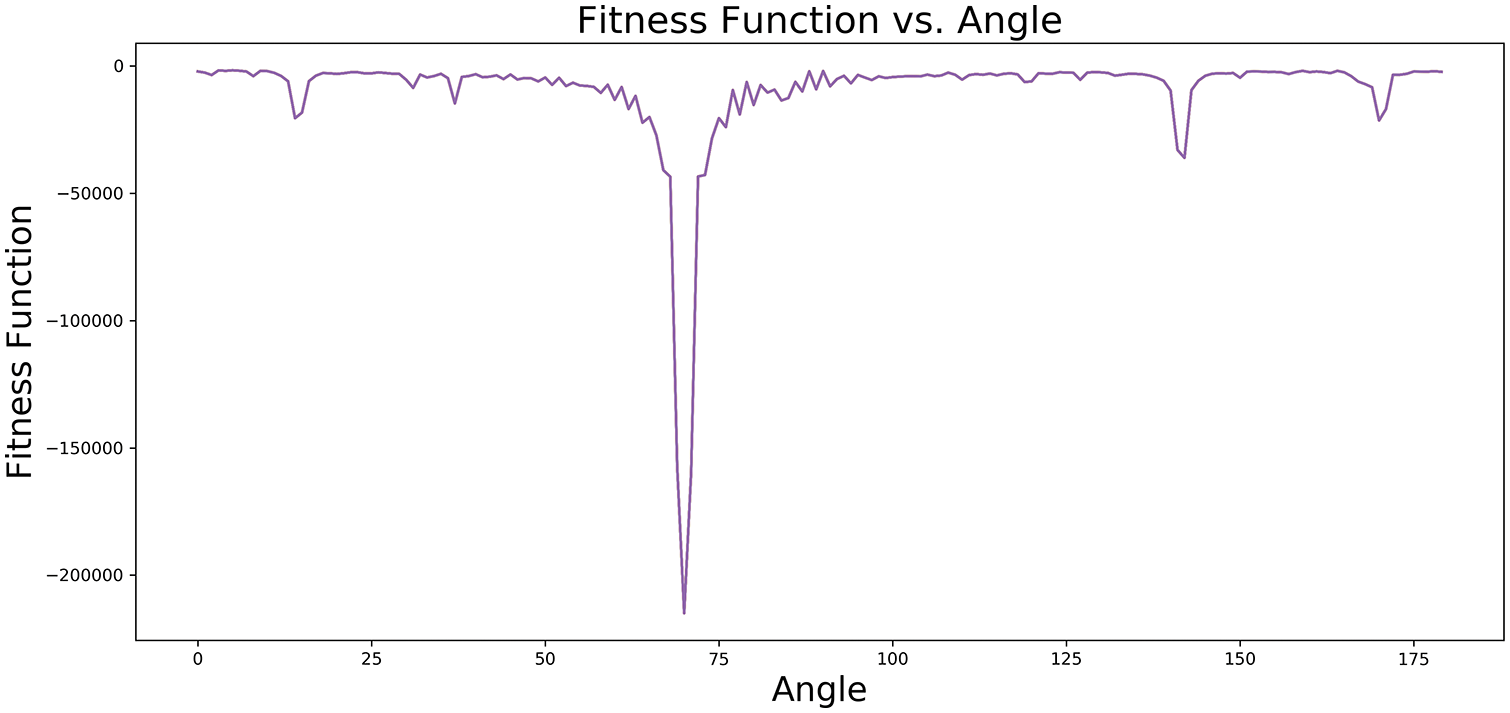
Figure 12: Fitness Function vs. θ. It has a global minimum at θ = 70 (the dominant angel)

4.1 Evaluation of the Noise Effect

One of the most important things related to any algorithm is its robustness against noise effects. This section, hankers for drawing a broad picture of the noise tolerance of our model. Fig. 13 represents an input directional image with its noisy version (An additive Gaussian noise with σ = 10). The Error image, which is defined as a differential image between two images, also is depicted in this experiment. The Error energy shows that the degrading effect of the additive Gaussian noise is so high. To make an appropriate compassion to Fig. 13, the experiment is repeated; but this time, the image space is replaced by the Radon space.

Figure 13: Image signal space: Input image vs. Noisy image vs. Error image

In Fig. 14, the Radon projection maps are depicted for the input image, its noisy version, and the Error image in the Radon space. When the noisy image in the signal space in Fig. 13 is compared with the noisy image in the Radon space in Fig. 14, it shows that in the Radon space, the information related to the orientation can still be extracted from the noisy image. In contrast, its corresponding noisy image in the signal space has almost no helpful information about the actual direction. It indeed means that the noise effect in the Radon space is much lower, and an appropriate estimator can spot a dominant orientation even with a high power noise.

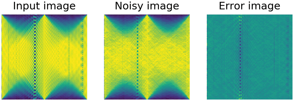
Figure 14: Radon signal space: Radon Transform of the input image vs. Noisy image vs. Error image

We compare the MSE2D, PSNR, and SSIM for the input image and the noisy image in both image signal space and Radon space to perform a more thorough analysis. Fig. 15 shows the MSE2D for two different spaces in various noise powers. In our implementations, the σ was increased from 0 to 65.

Figure 15: Comparing the MSE between the image signal space, and the Radon space

The figure indicates that the MSE2D−SS (the MSE in the signal space) is growing up exponentially with rising noise power. On the opposite side, MSE2D−RS (the MSE in the Radon space) is well below the corresponding values in the signal space with little variations of the MSE between σ = 0 to σ = 65.

In addition to the MSE, the PSNR is also illustrated in Fig. 16 for two different spaces. The achieved results show that there is a big gap between the PSNR in the signal space (PSNRSS) (the red line) and the PSNR in the Radon space (PSNRRS) (the blue line). Indeed, the PSNRSS is dominated by the PSNRRS. This indicates the Radon space keeps up the image quality rather than the signal space. Then, in order to remedy some of the issues associated with MSE and PSNR, SSIM is deployed. As mentioned, the SSIM value can vary between −1 and 1, where 1 indicates the perfect similarity. Fig. 17 compares the SSIM between the signal space and the Radon space for different values of the σ. The results unveil that SSIMRS (SSIM in the Radon space) decreased gradually from 1 to about 0.8 with increasing of the σ while SSIMSS (SSIM in the signal space) was diving sharply from 1 to almost 0 during similar noise conditions. This indicates the perfect similarity is more achievable in the Radon space rather than signal space, providing that an appropriate feature extraction procedure is available. It is worth mentioning that all inputs were normalized using Eq. (20) before computing the Error Image, MSE2D, PSNR, and SSIM.

xs=x−xminxmax−xmin(20)

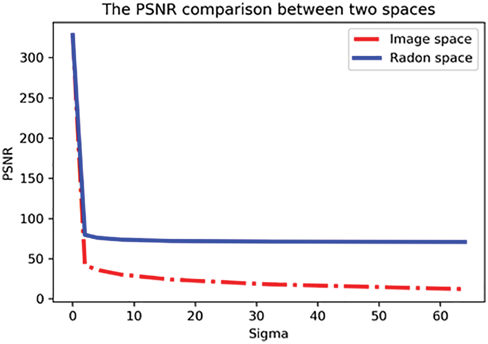
Figure 16: Comparing the PSNR between the image signal space and the Radon space

Figure 17: Comparing the SSIM between the image signal space and the Radon space

In Eq. (20), xS is the scaled version (the normalized version), and x is the input image (either in the signal space or the Radon space). Alongside, xmin and xmax are the minimum and maximum of the x, respectively.

In image processing problems where feature detection is the only need, mapping of an original image from image space to corresponding feature space via a useful transform, with subsequent processing in lower dimension feature space, would be an appropriate. Radon domain, when properly executed, can lead to minimum entropy or maximum sparseness. High-resolution Radon Transform methods can efficiently remove random or correlated noise, improve signal clarity, by utilizing the move-out or curvature of the signal of interest. This article has deployed 2D Mean Square Error (MSE2D), Peak Signal-to-Noise Ratio (PSNR), and Structural Similarity Measure (SSIM) to evaluate the accuracy of the proposed feature extraction algorithm. There are noticeable gaps between Red & Blue lines, corresponding to Image & Radon spaces for all three evaluation metrics. This indicates the proposed feature detection method is strong enough to benefit the Radon space potential characteristics, such as getting the least entropy or the most sparseness.

In a new scenario, the aim is to evaluate the noise power impact on the fitness function variations. In Fig. 18, several fitness functions are drawn for noisy images with σ = 0 (no noise) to σ = 11 with θ = 80. In almost all experiments, the fitness function has a global minimum of about θ = 80 (the perfect estimation). The second extremum is also highlighted in this figure. When the noise power increases sharply, a local minima may change and even be converted to a fake global minimum. This phenomenon will be investigated in the succeeding scenario. In Fig. 19, the skew and frequency of the synthetic input image are upgraded. In almost all curves for noisy images with σ = 0 (no noise) to σ = 9, the fitness function has a global minimum of about θ = 30. This means the estimator is doing magnificently even with a relatively high noise power. This indicates that the proposed approach tolerates noise effects marvelously. Now, the noise power increases, manifestly. Fig. 20, shows that when σ rises from 10 to 45, there is no longer a regular pattern. Besides, for the very high noise powers such as σ = 30, 40, and 45 the real extremums were flipped, and replaced by other false local minimums. As a result, in presence of the very high power additive Gaussian noise, the error can be grown sharply.

Figure 18: Comparing the fitness function vs. θ for noisy images from σ = 0 (no noise) to σ = 11 with the estimated θ^ = 80

Figure 19: Comparing the fitness function vs. θ for noisy images with σ = 0 (no noise) to σ = 9 with the estimated θ^ = 30

Figure 20: Comparing the fitness function vs. θ for noisy images with σ = 0 (no noise) to σ = 45

4.2 Computational Time

To reduce the run-time, the image size can be reduced by a scale factor α. This step can potentially speed up the processing time but it may lead to a reduction in the accuracy. As a result, in this section, the aim is to analyze the proposed re-scaling procedure effects on not only the run-time but also some critical algorithm’s performance measures such as the Accuracy, MSE, and MAE. For this purpose, a 65 × 65 synthetic image with θ = 70 is considered in Fig. 21. In this new experiment, the scaling factor (α) is selected from the set [1.0, 0.9, 0.7, 0.5], and α = 1 means there is no re-scaling procedure. Fig. 21 demonstrates that the global minimum of the fitness function has no drift due to the re-scaling procedure. Therefore, the estimator can detect the skew accurately for even α = 0.5 for a very tiny input image with the original size of 65 × 65. Then, the experiment is extended for a 600 × 600 synthetic image with θ = 70 at several scale factors, such as 1.0, 0.9, 0.7, 0.5, 0.4, 0.3, 0.15, and also 0.1. Similarly, the results are very satisfying even for α = 0.1 for the recent example (See Fig. 22).

Figure 21: The fitness function for a 65 × 65 synthetic image with θ = 70 at different scale factors

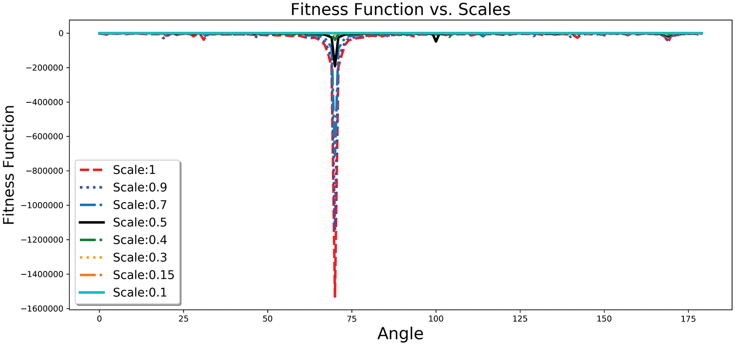
Figure 22: The fitness function for a 600 × 600 synthetic image with θ = 70 at different scale factors

To have more discussions, the outcomes of some new experiments are reported in both Tables 1, and 2. In these tables, α is the scale factor, Image size* is the size of the scaled image, θ is the dominant orientation of an input image, θ^ represents the estimated skew, Error =θ−θ^, while Time shows the run-time in the second. In Table 1, for all scale factors that range between 0.1, and 1, the estimation error would be precisely zero, while the computation time decreases from 3.16612 s for α = 1 (Image size* = 600 × 600) to just 0.08803 s for α = 0.1 (Image size* = 60 × 60). This means the proposed Radon CLF is not only an accurate algorithm but also can reduce the run-time blatantly. In Table 2, the error would be zero except for α = 0.3, with a remarkably tiny image including only 20 rows and 20 columns of pixels. In this table, the estimation error is still zero for any Image size* greater than 20 × 20. This implies that any more reduction of the input size can increase the probability of the error. Furthermore, Table 2 denotes that with re-scaling the input image from its original size of 65 × 65 to 26 × 26, the run-time falls from 0.09996 s to 0.04103, and at the same time, there is still no error.

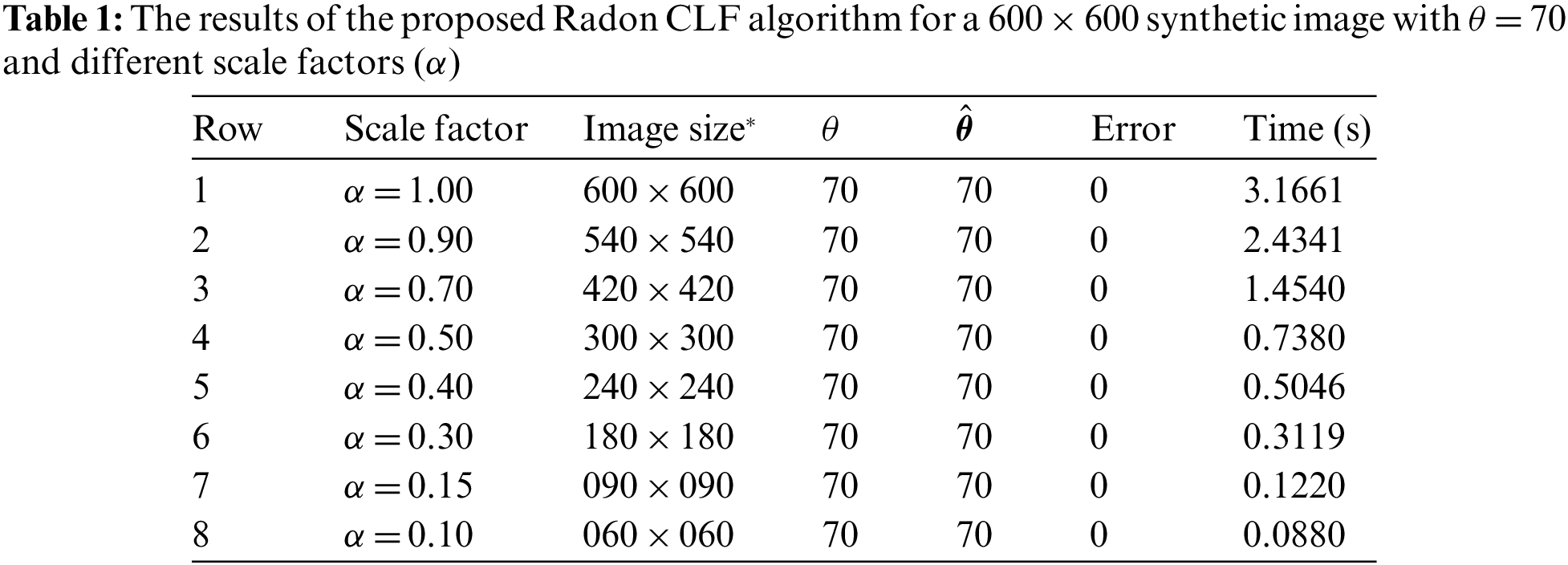
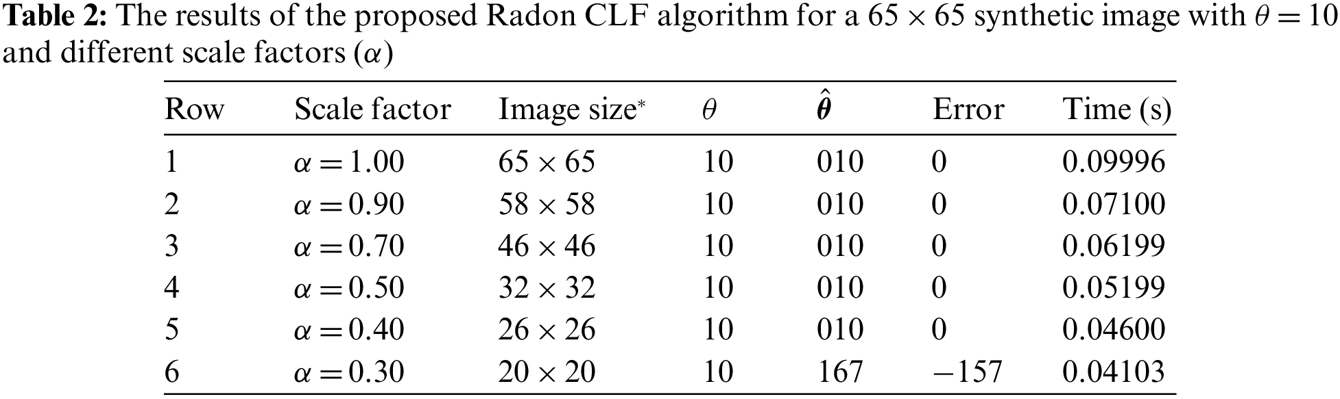
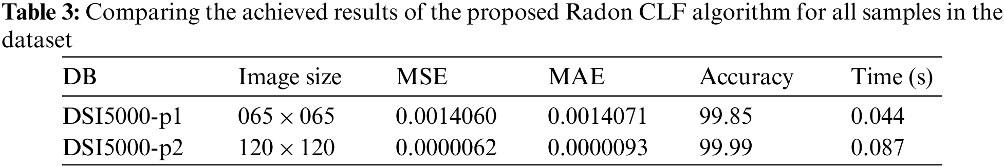
Table 3 shows the achieved results due to running the Radon CLF algorithm on about 5696 images in the DSI5000 dataset. The dataset has been divided into two parts named DSI5000-p1 and DSI5000-p2. Each part has an equal number of samples, around 2848 images. According to Table 3, the DSI5000-p1 includes images with a lower size (65 × 65). In comparison with the DSI5000-p2, the DSI5000-p1 has a lower run-time together with a lower accuracy.

In addition to DSI5000, many real-world scanned image documents were also included in our simulations. Both handwriting, and printed samples, at various resolutions, were gathered from different Persian/Arabic & English multilingual resources such as books, booklets, letters, and newspapers. Fig. 23 shows some samples and the result of the Radon CLF algorithm. Our method can accurately detect the skew in real photos, according to experimental results.

Figure 23: Examination of the proposed algorithm on real documents

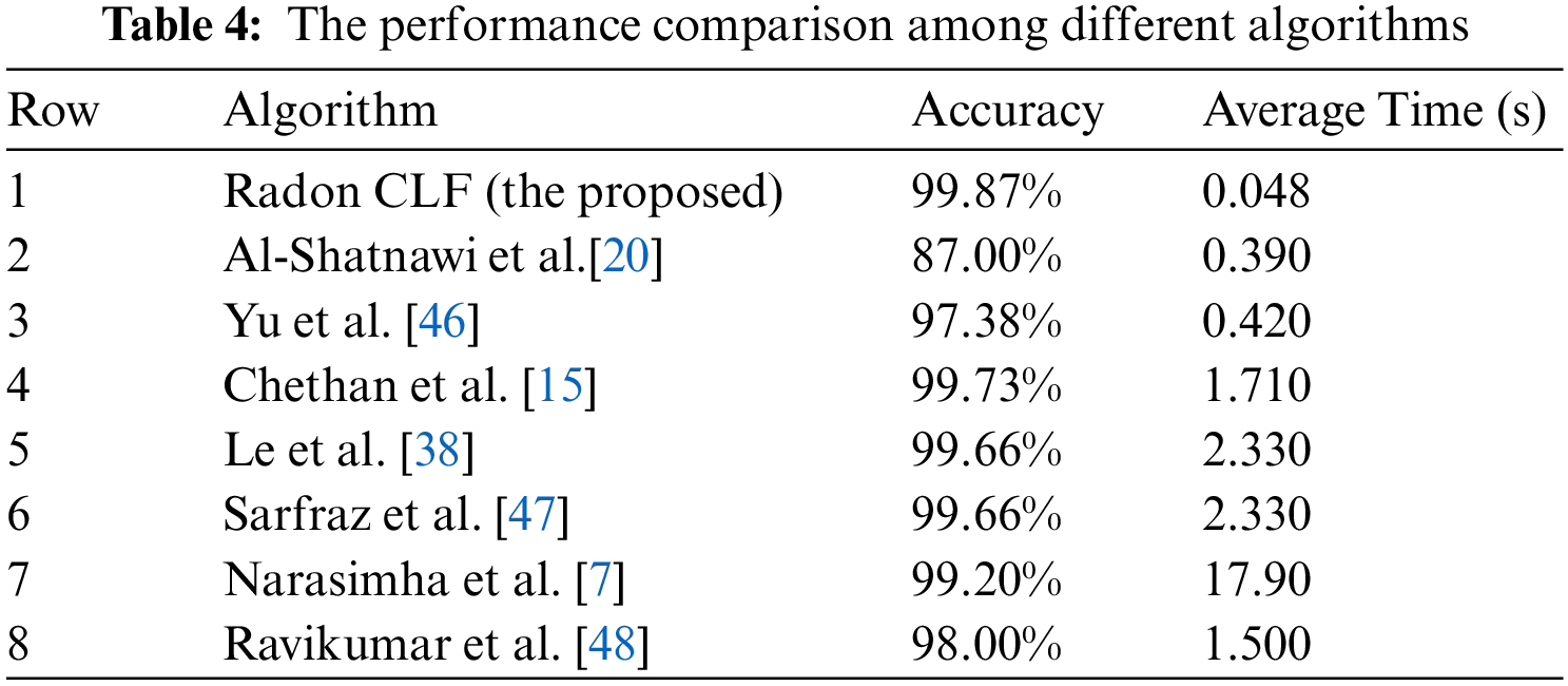
Finally, Table 4 draws a comparison between the proposed approach and other available algorithms. Experimental results show that our algorithm is capable of skew compensating for large documents far faster than well-known existing methods, with a run-time of about 0.048 s and an Accuracy of 99.87% for DSI5000 dataset.

5  Conclusion and Future Works

In this paper, we proposed a novel, fast, and reliable skew detection algorithm for text images based on the Radon Transform and Curve Length Fitness Function (CLF). In addition, approximately 5696 synthetic images were incorporated into a new dataset called DSI5000. Many real image documents were also included in our simulations along with synthetic images. From various Persian, Arabic, English, and multilingual sources, random handwriting and printed samples of some books, booklets, letters, and newspapers, were collected at different resolutions.

The resilience of signal and image processing algorithms against noise effects is one of the most crucial issues. Through the utilization of many performance indicators, such as accuracy, MSE, MAE, PSNR, SSIM, and error signal comparison in both the signal space and the Radon space, we have created a detailed picture of the noise tolerance of our model in this study. Our approach is superior to other existing methods in terms of accuracy as well as timing efficiency, as shown by the results with the Accuracy of about 99.87% & run-time of around 0.048 (s) for DSI5000 dataset. For multilingual manuscripts with various font types, sizes, and styles, the suggested Radon CLF approach could find skews between 0° and 90°.

Machine Learning (ML) is a fast-growing and interesting field of applied research with high demands in scientific communities and advanced technologies. Deep Learning (DL) is a branch of ML that makes use of Artificial Neural Networks (ANN) to simulate how the human brain learns [49–51]. In the future, we intend to utilize DL models. They can be used to develop Radon CLF method for other computer vision applications, such as Camera Rotations Automatic Recovery, Rotation estimation in the urban environment, Fingerprint Recognition etc., which are particularly sensitive to directional patterns. Directional patterns have two main attributes: Dominant Orientation and Frequency. In our future studies, we will focus more on the joint estimation of both features using deep learning and Radon CLF.

Funding Statement: There are no sources of funding that have supported this work.

Conflicts of Interest: The authors declare that they have no conflicts of interest to report regarding the present study.

References

1. A. Chaudhuri, K.Mandaviya, P. Badelia and S. K. Ghosh, Optical Character Recognition Systems for Different Languages with Soft Computing, vol. 352. New York,USA: Springer, pp. 9–41, 2017. [Google Scholar]

2. M. Khorsheed, “Offline recognition of omni font Arabic text using the HMM ToolKit (HTK),” Pattern Recognition Letters, vol. 28, no. 12, pp. 1563–1571, 2007. [Google Scholar]

3. B. V. Dhandra, V. S. Malemath and H. Mallikarjun, “Skew detection in binary image documents based on image dilation and region labeling approach,” in 18th Int. Conf. on Pattern Recognition (ICPR’06),Hong Kong, China, pp. 954–957, 2006. [Google Scholar]

4. H. Dehbovid, F. Razzazi and S. Alirezaii, “A novel method for de-warping in Persian document images captured by cameras,” in 2010 Int. Conf. on Computer Information Systems and Industrial Management Applications (CISIM), Krakow, Poland, pp. 614–619, 2010. [Google Scholar]

5. T. Nawaz, S. Naqvi, H. Rehman and A. Faiz, “Optical character recognition system for Urdu (Naskh font) using pattern matching technique,” International Journal of Image Processing (IJIP), vol. 3, no. 3, pp. 92–104, 2009. [Google Scholar]

6. R. Salagar, “Analysis of PCA usage to detect and correct skew in document images,” in Information and Communication Technology for Competitive Strategies, vol.191. New York, USA: Springer, pp. 687–695, 2022. [Google Scholar]

7. R. S. Narasimha and S. D. Parag, “A novel local skew correction and segmentation approach for printed multilingual Indian documents,” Alexandria Engineering Journal, vol. 57, no. 3, pp. 1609–1618, 2018. [Google Scholar]

8. M. Pechwitz and V. Margner, “Baseline estimation for Arabic handwritten words,” in Proc. Eighth Int. Workshop on Frontiers in Handwriting Recognition, Niagra-on-the-Lake, ON, Canada, pp. 479–484, 2002. [Google Scholar]

9. Y. Zhang, Z. Huang, S. Jin and L. Cao, “Hough transform-based multi-object autofocusing compressive holography,” Applied Optics, vol. 62, pp. 23–30, 2023. [Google Scholar]

10. S. Kumar and K. Karibasappa, “An approach for brain tumour detection based on dual-tree complex Gabor wavelet transform and neural network using Hadoop big data analysis,” Multimedia Tools and Applications, vol. 81, pp. 39251–39274, 2022. [Google Scholar]

11. P. Mukhopadhyay and B. B. Chaudhuri, “A survey of Hough transform,” Pattern Recognition, vol. 48,no. 3, pp. 993–1010, 2015. [Google Scholar]

12. Z. Chen and L. Zhang, “Multi-stage directional median filter,” International Journal of Signal Processing, vol. 5, no. 4, pp. 249–252, 2009. [Google Scholar]

13. M. Bahaghighat, F. Abedini, Q. Xin, M. M. Zanjireh and S. Mirjalili, “Using machine learning and computer vision to estimate the angular velocity of wind turbines in smart grids remotely,” Energy Reports, vol. 7, pp. 8561–8576, 2021. [Google Scholar]

14. Y. Y. Tang, S. W. Lee and C. Y. Suen, “Automatic document processing: A survey,” Pattern Recognition, vol. 29, no. 12, pp. 1931–1952, 1996. [Google Scholar]

15. H. K. Chethan and G. H. Kumar, “Graphics separation and skew correction for mobile captured documents and comparative analysis with existing methods,” International Journal of Computer Applications, vol. 7, no. 3, pp. 42–47, 2010. [Google Scholar]

16. P. V. Bezmaternykh and D. P. Nikolaev, “A document skew detection method using fast Hough transform,” in Twelfth Int. Conf. on Machine Vision (ICMV 2019), Amsterdam, Netherlands, vol. pp. 11433, pp. 132–137, 2020. [Google Scholar]

17. L. Y. Chiu, Y. Y. Tang and C. Y. Suen, “Document skew detection based on the fractal and least squares method,” in Proc. of 3rd Int. Conf. on Document Analysis and Recognition, Montreal, QC, Canada, vol. 12, pp. 1149–1152, 1995. [Google Scholar]

18. P. Shivakumara, D. S. Guru, K. Hemantha and P. Nagabhushan, “A novel technique for estimation of skew in binary text document images based on linear regression analysis,” Sadhana, vol. 30, no. 1, pp. 69–85, 2005. [Google Scholar]

19. P. Shivakumara, K. Hemantha, D. S. Guru and P. Nagabhushan, “Skew estimation of binary document images using static and dynamic thresholds useful for document image mosaicking,” in National Workshop on IT Services and Applications (WITSA), New Delhi, India, pp. 27–28, 2003. [Google Scholar]

20. A. Al-Shatnawi and K. Omar, “Skew detection and correction technique for Arabic document images based on centre of gravity,” Journal of Computer Science, vol. 5, no. 5, pp. 363–368, 2009. [Google Scholar]

21. T. Jundale, R. Hegadi and S. Ravindra, “Skew detection and correction of Devanagari script using Hough transform,” Procedia Computer Science, vol. 45, pp. 305–311, 2015. [Google Scholar]

22. R. Singh and R. Kaur, “Improved skew detection and correction approach using Discrete Fourier algorithm,” International Journal of Soft Computing and Engineering, vol. 3, no. 4, pp. 5–7, 2013. [Google Scholar]

23. Y. Lu and C. L. Tan, “A nearest-neighbor chain based approach to skew estimation in document images,” Pattern Recognition Letters, vol. 24, no. 14, pp. 2315–2323, 2003. [Google Scholar]

24. R. Chang, “Application of principal component analysis in image signal processing,” in Proc. Int. Conf. on Image, Signal Processing, and Pattern Recognition (ISPP 2022), Guilin, China, pp. 12–24, 2022. [Google Scholar]

25. W. Bao, C. Yang, S. Wen, M. Zeng, J. Guo et al., “A novel adaptive deskewing algorithm for document images,” Sensors, vol. 22, no. 20, pp. 7944–7962, 2022. [Google Scholar] [PubMed]

26. Y. L. Chaitra and R. Dinesh, “An impact of radon transforms and filtering techniques for text localization in natural scene text images,” in ICT with Intelligent Applications, vol. 248. New York, USA: Springer, pp. 563–573, 2022. [Google Scholar]

27. P. C. Theofanopoulos, M. Sakr and G. C. Trichopoulos, “Multistatic terahertz imaging using the Radon transform,” IEEE Transactions on Antennas and Propagation, vol. 67, no. 4, pp. 2700–2709, 2019. [Google Scholar]

28. L. J. Nelson and R. A. Smith, “Fibre direction and stacking sequence measurement in carbon fibre composites using Radon transforms of ultrasonic data,” Composites Part A: Applied Science and Manufacturing, vol. 118, pp. 1–8, 2019. [Google Scholar]

29. G. Beylkin, “Discrete radon transform,” IEEE Transactions on Acoustics, Speech, and Signal Processing, vol. 35, no. 2, pp. 162–172, 1987. [Google Scholar]

30. S. Aftab, S. F. Ali, A. Mahmood and U. Suleman, “A boosting framework for human posture recognition using Spatio-temporal features along with radon transform,” Multimedia Tools and Applications, vol. 81, pp. 42325–42351, 2022. [Google Scholar]

31. C. Grathwohl, P. C. Kunstmann, E. T. Quinto and A. Rieder, “Imaging with the elliptic Radon transform in three dimensions from an analytical and numerical perspective,” SIAM Journal on Imaging Sciences, vol. 13, no. 4, pp. 2250–2280, 2020. [Google Scholar]

32. S. Chelbi and A. Mekhmoukh, “Features based image registration using cross-correlation and Radon transform,” Alexandria Engineering Journal, vol. 57, no. 4, pp. 2313–2318, 2018. [Google Scholar]

33. Q. Zhang, “Automated road network extraction from high spatial resolution multi-spectral imagery,” Ph.D. Dissertation, University of Calgary, Canada, 2006. [Google Scholar]

34. J. S. Seo, J. Haitsma, T. Kalker and C. D. Yoo, “A robust image fingerprinting system using the Radon transform,” Signal Processing: Image Communication, vol. 19, no. 4, pp. 325–339, 2004. [Google Scholar]

35. V. Kiani, R. Pourreza and H. R. Pourreza, “Offline signature verification using local radon transform and support vector machines, ” International Journal of Image Processing, vol. 3, no. 5, pp. 184–194, 2009. [Google Scholar]

36. M. Beckmann, A. Bhandari and F. Krahmer, “The modulo Radon transform: Theory, algorithms, and applications,” SIAM Journal on Imaging Sciences, vol. 15, no. 2, pp. 455–490, 2022. [Google Scholar]

37. S. H. Mohana and C. J. Prabhakar, “Stem-Calyx recognition of an apple using shape descriptors,” Signal & Image Processing : An International Journal (SIPIJ), vol. 5, no. 6, pp. 17–31, 2014. [Google Scholar]

38. D. S. Le, G. R. Thoma and H. Wechsler, “Automated page orientation and skew angle detection for binary document images,” Pattern Recognition, vol. 27, no. 10, pp. 1325–1344, 1994. [Google Scholar]

39. S. Chikkerur, A. N. Cartwright and V. Govindaraju, “Fingerprint enhancement using STFT analysis,” Pattern Recognition, vol. 40, no. 1, pp. 198–211, 2007. [Google Scholar]

40. U. Sara, M. Akter and M. S. Uddin, “Image quality assessment through FSIM, SSIM, MSE and PSNR—A comparative study,” Journal of Computer and Communications, vol. 7, no. 3, pp. 8–18, 2019. [Google Scholar]

41. Z. Cui, Z. Gan, G. Tang, F. Liu and X. Zhu, “Image signature based mean square error for image quality assessment,” Chinese Journal of Electronics, vol. 24, no. 4, pp. 755–760, 2015. [Google Scholar]

42. M. Bahaghighat, S. A. Motamedi and Q. Xin, “Image transmission over cognitive radio networks for smart grid applications,” Applied Sciences, vol. 9, no. 24, pp. 5498–5529, 2019. [Google Scholar]

43. G. Corona, O. Maciel-Castillo, J. Morales-Castañeda and A. Gonzalez, “A new method to solve rotated template matching using metaheuristic algorithms and the structural similarity index,” Mathematics and Computers in Simulation, vol. 206, pp. 130–146, 2023. [Google Scholar]

44. R. Bhatt, N. Naik and V. K. Subramanian, “SSIM compliant modeling framework with denoising and deblurring applications,” IEEE Transactions on Image Processing, vol. 30, pp. 2611–2626, 2021. [Google Scholar] [PubMed]

45. S. Bafjaish, M. S. Azmi, M. N. Al-Mhiqani, A. R. Radzid and H. Mahdin, “Skew detection and correction of Mushaf Al-Quran script using hough transform,” International Journal of Advanced Computer Science and Applications, vol. 9, no. 8, pp. 402–409, 2018. [Google Scholar]

46. B. Yu and A. K. Jain, “A robust and fast skew detection algorithm for generic documents,” Pattern Recognition, vol. 29, no. 10, pp. 1599–1629, 1996. [Google Scholar]

47. M. Sarfraz, S. A. Mahmoud and Z. Rasheed, “On skew estimation and correction of text, computer graphics,” in Proc. of Computer Graphics, Imaging and Visualization Conf. (CGIV 2007), Bangkok, Thailand, pp. 308–313, 2007. [Google Scholar]

48. M. Ravikumar and O. A. Boraik, “Estimation and correction of multiple skew Arabic handwritten document images,” International Conference on Innovative Computing and Communications, vol. 1387, pp. 553–564, 2022. [Google Scholar]

49. A. Hajikarimi and M. Bahaghighat, “Optimum outlier detection in internet of things industries using autoencoder,” in Frontiers in Nature-Inspired Industrial Optimization, New York, USA: Springer, pp. 77–92, 2022. [Google Scholar]

50. A. M. Hilal, A. Al-Rasheed, J. S. Alzahrani, M. M. Eltahir and M. A. Duhayyim, “Competitive multi-verse optimization with deep learning based sleep stage classification,” Computer Systems Science and Engineering, vol. 45, no. 2, pp. 1249–1263, 2023. [Google Scholar]

51. M. J. Umer, M. Sharif, M. Alhaisoni, U. Tariq and Y. J. Kim, “A framework of deep learning and selection-based breast cancer detection from histopathology images,” Computer Systems Science and Engineering, vol. 45, no. 2, pp. 1001–1016, 2023. [Google Scholar]