Evolution Performance of Symbolic Radial Basis Function Neural Network by Using Evolutionary Algorithms

1  Introduction

In various scientific and engineering fields, many scholars were fascinated by the Radial Basis Function Neural Network (RBFNN) due to the network’s simple structure, fast learning speed, as well as the network’s enhanced capabilities of approximation. RBFNN represents a feed-forward neural network with containing three layers of neurons: (1) an input layer, (2) a hidden layer, and (3) an output layer. The input neurons in the 1st layer receive data, then they transfer the data to the specified hidden layer to carry out data training and synthesis. In the hidden layer will calculate the width and the center for all neurons between the input data and the prototype stored inside it, using the Gaussian activation function. This synthesized information can be employed in the mentioned output layer, which contains output neurons. These three layers minimize the classification errors, as well as the prediction errors in RBFNN [1]. Hamadneh et al. [2], who first applied the logical rule of logic programming in RBFNN, explored the Horn Satisfiability logic programming (HornSAT) credibility. Therefore, the RBFNN logical structure is uniquely dependent on three parameters only, including the entire input neurons center, widths, as well as the Gaussian activation function. Despite the efficiency of applying RBFNN within the RBFNN’s hidden layer, the number of these neurons can determine the network’s complexity [3]. Regarding the network’s hidden layer, when the neurons number is insufficient, the learning within the network of RBFNN will not achieve the best convergence; however, when there are enough neurons, the network will experience overlearning [4].

In a study by Yang et al. [5], the authors effectively applied the method of the Sparse Neural Network (SNN) so that the hidden neurons are increased. The goal of the SNN paradigm involves reducing the resultant error by using the trial-error mechanism to define the hidden neuron numbers clearly from a specified neuron group. However, the limitation of the SNN paradigm involves the substantial computational time throughout the hidden neurons number computation processes as inspired by previous studies [6–8], whereby the 2 Satisfiability (2SAT) logic representation has been used with the RBFNN so that crucial parameters in the hidden layer are determined, thereby controlling these hidden neurons. Accordingly, 2SAT has been selected because it complies with the RBFNN’s structure and representation.

2  Literature Review

The complexity of SRBFNN-2SAT increases when the clauses number increases, and therefore, this optimization algorithm is essential. Global optimization methods have been applied widely due to their global search capabilities. The metaheuristics algorithm represents a widespread algorithm used in searching the RBFNN near-optimal solution [9,10]. There are various nature-inspired algorithms, as well as improved optimization algorithms, including Evolutionary Algorithms (EA), which are suitable for countless problems of engineering optimization [11]. Another essential 2SAT constituent in RBFNN is the effective training method, which affects the performance of the SRBFNN-2SAT. This study aims to establish an array of diverse Evolutionary Algorithms involving the Genetic Algorithm (GA) [12], Evolution Strategy (ES) [13], Differential Evolution (DE) [14], and Evolutionary Programming (EP) [15].

The theoretical foundation of the Genetic Algorithm (GA) was developed by Holland [12], who first applied GA to solve problems which controlled the transmission of gas-pipeline Goldberg et al. [16]. Hamadneh et al. [2] employed GA so that the RBFNN-hybrid model could be trained using a higher-order SAT logic. They utilized GA and k-means cluster algorithms for training the RBFNN with a higher-order Logic Programming Satisfiability. Pandey et al. [17] endeavored to obtain the optimal algorithm by comparing the Multiple Linear Regression (MLR) through a specified genetic method for forecasting the temporal scour depth near-circular pier in non-cohesive sediment. The authors used 1100 exploratory laboratory datasets for optimizing the generalized scour Equation using GA and MLR. In a recent study, Jing et al. [18] improved an innovative reliability analysis method using a combination of GA-RBFNN. GA has been implemented in this paper for determining the most potential or most probable point (MPP) in a specific optimization problem via controlling the resulting density of the tested samples for refining RBFNN.

During the late 1960s, an ES Algorithm was developed by Rechenberg [13] with a deterministic step size control. He established convergence with the achieved rate of convergence in ES. Several attempts have been made to apply the ES algorithm to multimodal function optimization. In this regard, Moreira et al. [19] assessed ES when the authors compared the algorithm’s performance with GA. The results established that the ES algorithm showed effectiveness and robustness. ES was also used by Fernandes et al. [20] for pruning Generative Adversarial Networks (GANs). The results showed that this pruned model of the GAN with ES achieved the most efficient performance compared with GAN’s original model. On other hand, Karabulut et al. [21] attempted to find the optimal algorithm. The researchers used the ES Algorithm to solve multiple traveling salesman problems. The computational outcomes showed that this algorithm could find the optimum solution to all Traveling Salesman Problems.

Storn et al. [14] are the first scholars who have introduced the DE Algorithm for solving various global optimization problems. The DE Algorithm is a manageable and robust evolutionary algorithm that uses fewer parameters with greater simplicity and faster convergence [14]. The use of the DE Algorithm with other algorithms proved effective, specifically with the Hopfield Neural Network [22], as well as feed-forward neural networks [23]. DE was also utilized by Tao et al. [24] for improving RBFNN in a specific prediction model for the cooking energy consumption process. This projected model can classify problems and solve function approximations using better accuracy and improved generalization capabilities. The outcomes showed that DE could optimize RBFNN with higher accuracy [24].

The theoretical foundation of the EP Algorithm has been improved by Fogel et al. [15]. In their study, the authors have improved the artificial intelligence evolution’s capability of changing predictions in an environment. Similarly, Singh et al. [25] improved EP for tackling the problem of multi-fuel economic load dispatch. EP, which depends on Powell’s pattern search, demonstrated effectiveness in obtaining better convergence characteristics and achieving the most optimum solution. Tian et al. [26] have recently proposed EP for learning processes of Convolutional Neural Network (CNN) model-building. The EP algorithm-based CNN reached the most optimal solutions effectively. The implementation of EP in various combinatorial and numerical optimization problems has shown effectiveness because faster convergence rates were obtained; however, the use of the EP Algorithm showed effectiveness for only a few function optimization problems [27].

The proposed work in this paper differs from the others’ work in several aspects. The main differences are as follows:

1.    Diverse Evolutionary Algorithms (EAs) involving GA, ES, DE, and EP was pioneered in this paper by comparing the EAs to facilitate the training of Symbolic Radial Basic Function Neural Network (SRBFNN) using several performance metrics. These include Root Mean Square Error (RMSE), Mean Absolute Relative Error (MARE), Mean Absolute Percentage Error (MAPE), Systematic Error (SD), Mean Bias Error (MBE), Central Process Unit time (CPU time), and Schwarz Bayesian Criterion (SBC). The EP algorithm efficiently complied in tandem with SRBFNN.

2.    The objective of this paper has been motivated by the features of EAs; these were not considered by other work and researchers to train Symbolic Radial Basic Function Neural Network (SRBFNN) beside logic programming. Moreover, a comprehensive investigation of the potential effects of various EAs has been provided in this work, which aims to train the SRBFNN to execute logic programming 2SAT by using many performance metrics. By utilizing the SRBFNN with logic programming 2SAT, the EAs’ effects were examined in one framework only in the training phase. Besides, a comparison has been conducted in this paper among the proposed algorithms so that the optimum algorithm is selected. The selected algorithm can train SRBFNN-2SAT. These aspects were not investigated by other work and researchers. The primary purpose of utilizing various EAs is as follows:

1.    Increased flexibility. The concepts of EA have been adapted and modified to tackle the most sophisticated problems encountered by humans and achieve the desired objectives [28].

2.    Better optimization, whereby the massive “population” of the total potential solutions has been considered. In other words, algorithms cannot be restricted to a specified solution [29].

3.    Unlimited solutions. Unlike orthodox methods, which were presented and attempted to accomplish one optimum solution, evolutionary algorithms can provide various potential solutions to solve problems [30].

To this end, the contribution of this paper involves embedding different evolutionary algorithms to train SRBFNN-2SAT. This can be attributed to the proposed SRBFNN training, as it frequently converges to a given suboptimal output weight. In this study, the capability of EAs has been explored by conducting a comparison with other algorithms. Obtaining the optimum output weight and a lower iteration error is the primary goal of this training model in the SRBFNN-2SAT. Furthermore, extensive experimentation using a variety of performance metrics in this paper was conducted to determine the effectiveness of evolutionary algorithms in the training of SRBFNN-2SAT.

3  Radial Basis Function Neural Network (RBFNN)

RBFNN is a single variant of the variants of feed-forward neural networks that utilize the hidden-interconnected layer suggested by Lowe and Moody [31,32]. In contrast with different networks, the RBFNN network enjoys a combined structure and architecture [33]. There are three neuron layers in RBFNN to fulfill computation purposes. In the input layer, input data are transferred by the m neurons into the system. During a training phase, parameters, including (center, as well as width) is determined in the hidden layer of the RBFNN. These parameters can be utilized for determining the output weight in the RBFNN output layer, and the Gaussian activation function for the RBFNN hidden neuron [34,35] reduces dimensionality from the RBFNN’s input layer towards the output layer [34]:

Q(x)=‖∑i=1jwji′xi−ci‖22σi2(1)

φi(x)=e−Q(x)(2)

where ci, σi signify the given center of the specified hidden neuron, in addition to width, correspondingly and xi denotes a specified input value of the N input neurons and the Euclidean norm from a specified input neuron, i.e., i to the specified hidden neuron, i.e., j is given as follows [35]:

‖∑i=1jwji′xi−ci‖=∑m=1N(∑i=1jwji′xi−ci)2(3)

wherein wji′ denotes a specified input weight between the given input neuron, i.e., j with the given hidden neuron, i.e., i; the xi structurally constitutes the input data in a specified training set, as well as a specified hidden neuron, i.e., i while ci denotes a hidden neuron’s center. The RBFNN final predictor output F(wi) is provided herein [36]:

F(wi)=∑i=1jwiφi(xk)(4)

where F(wi) represents the RBFNN output value; a specified output weight is provided here wi. Thus, the RBFNN aims at obtaining the optimal weights, i.e., wi, thereby satisfying the needed output value, wherein the RBFNN hidden neuron carries out multiple functions, thereby signifying an input pattern spanned by the hidden neuron of RBFNN [2,33].

4  Symbolic Radial Basis Function Neural Network (SRBFNN-2SAT)

Two Satisfiability (2SAT) is a logic programming involved in 2 literals in one clause. The 2SAT logic programming determines if the given 2-Conjunctive Normal Form (2-CNF) has a satisfying assignment. 2SAT has been chosen in this paper due to converging satisfiability logic programming as 2 literals per clause at a time. 2SAT offers a better learning rule in RBFNN. As a specific logical rule, logic programming 2SAT has been applied in different disciplines, including industrial automation and sophisticated management systems. Many previous studies on logic programming 2SAT and neural networks were conducted [8,37]. The dataset information in this paper is characterized as 2SAT variables, representing an Artificial Neural Network (ANN) symbolic rule. Regarding this work, 2SAT is the primary driver as logical programming ensures that this program considers two literals only for every item for each implementation. It has been confirmed by previous studies that combinatorial problems can be formulated by applying 2SAT logic [3,35]. The primary reason behind the appropriateness of 2SAT logic to represent the neural network’s logical rules involves the selection of 2 literals only for each of the clauses within the Satisfiability logic, thereby reducing logical complexity in the relationships among variables in a neural network. Logic programming 2SAT has been selected in this study due to its compliance with the RBFNN based on its structure and representation. 2SAT is embedded into RBFNN by applying a specified variable as an input neuron, and every single neuron xi indicates {0,1}, in other words, False-True values. Upon utilizing this value of the input neuron, parameters ci and width will be calculated. The best-hidden neuron number will be achieved by embedding 2SAT as a specific logical rule that can make RBFNN receive additional input data by fixed width and center value. This combination aims to produce a model of RBFNN; this model can classify data according to the logical rule of 2SAT. The formula that provides the 2SAT representation in RBFNN is as follows [35]:

P2SAT=∨i=1kAi∨j=1nBj(5)

whereby k, n is natural number. Ai and Bj represent atoms. This paper restricted the number of literals to two. k, n = 2 for each Ai and Bj, named as 2 Satisfiability (2SAT) logical rule, P2SAT which is governed by Eq. (6) [8]:

P2SAT=(A∨B)∧(¬C∨D)∧(E∨¬F)(6)

where ∧ represents the conjunction (AND), ¬ signifies the negation of the literal, and ∨ represents the Disjunction (OR). Eqs. (6) and (7) are effectively used in determining the training data regarding each of the 2SAT clauses. Accordingly, implementing 2SAT in the RBFNN network is referred to as SRBFNN-2SAT. Table 1 illustrates the SRBFNN-2SAT input data form, as well as training random data as follows [35]:

xi=∑i=1kI(Ai)+∑j=1nI(Bj)(7)

whereby xi is the Input data in input layer during the training.

I(Ai)orI(Bj)={1,whenAorBisTrue0,whenAorBisFalse(8)

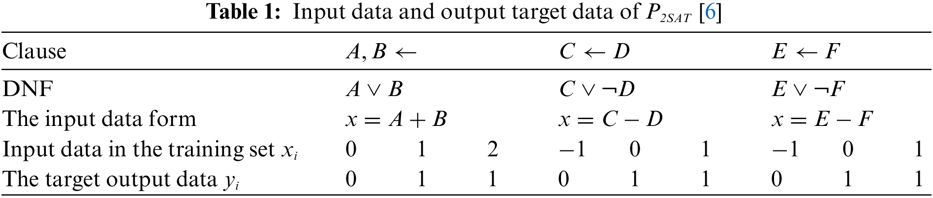
Based on Table 1, explain Eqs. (6) and (7) that are used in determining the training data and the target output regarding each of the 2SAT clauses and implementing 2SAT in the RBFNN network is referred to as SRBFNN-2SAT. A, B, C, D, E and F demonstrate the Disjunctive Normal Form (DNF) variables, input data xi is employed for calculating parameters involving center ci and width σi in the specified hidden layer. Where yi signifies the target logic programming output, which is utilized to find the SRBFNN-2SAT output weight. The 2SAT formulation is exemplified in the Conjunctive Normal Form (2CNF), and the CNF Satisfiability nature is conserved compared to other forms, such as the Disjunctive Normal Form (DNF). After locating the hidden layer’s width and center, RBFNN will use the Gaussian function in Eq. (1) for the output weight calculation. As the clauses number increases, SRBFNN-2SAT needs a more effective learning method for detecting the proper output weight. A metaheuristics algorithm has been performed in this work to identify the ideal output weights, thereby reducing the subsequent objective function as follows [34]:

f2SAT(wi)=∑i=1jwiφi(x)(9)

whereby f2SAT(wi) refers to the SRBFNN-2SAT ultimate output classification, and wi∈R represents the output weight in a hidden neuron in a hidden layer with an output neuron in an output layer. Where φi(x) is the Gaussian activation function in SRBFNN-2SAT, and j signifies a given hidden neuron number. Fig. 1 outlines the methodology flowchart.

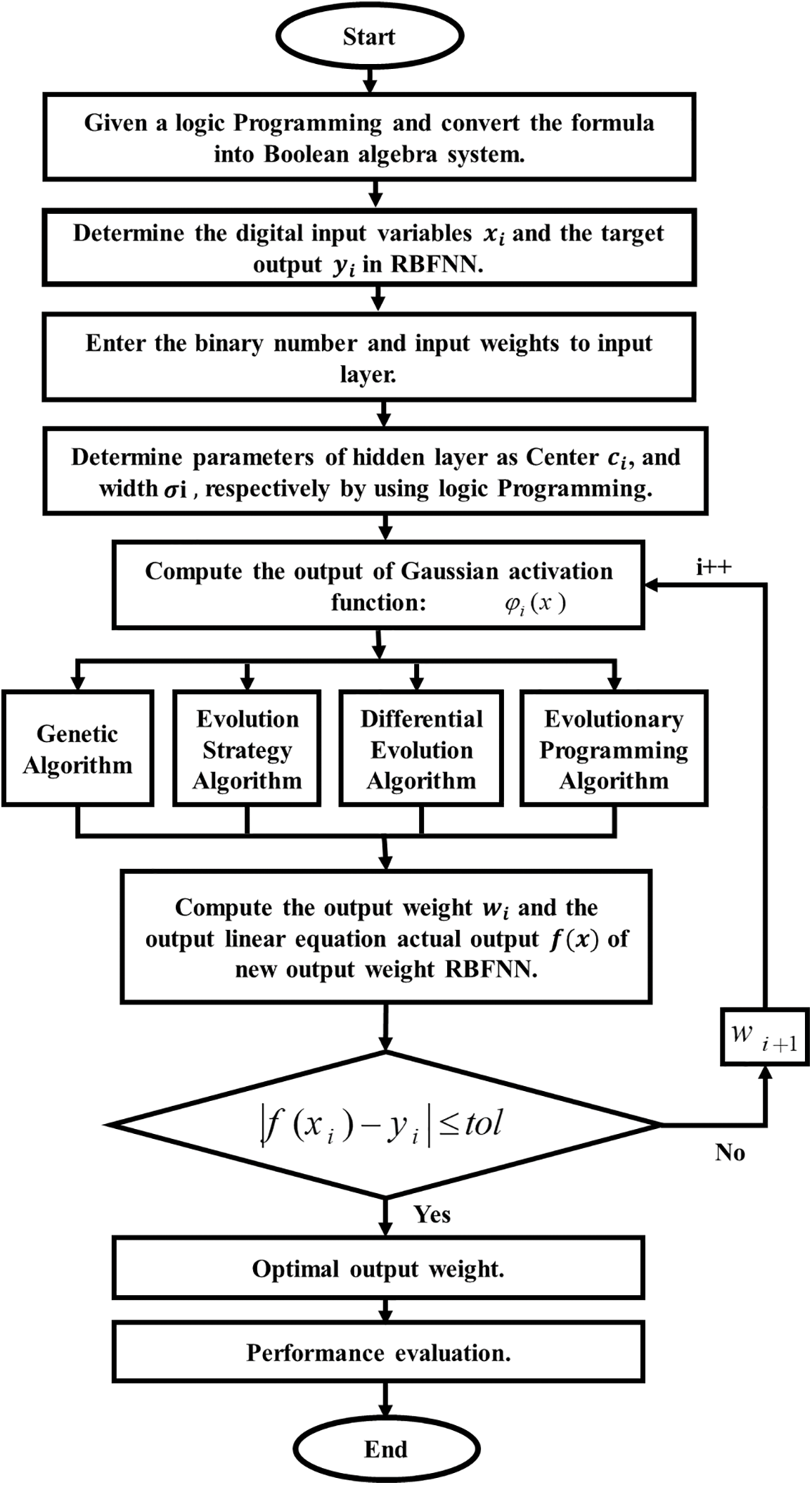
Figure 1: Methodology flowchart

SRBFNN-2SAT aims to achieve the optimum weights wi, thereby satisfying the needed RBFNN output value, and a group of functions can be provided by a hidden neuron, signifying an input pattern, which is spanned by the utilized hidden neuron [3,35]. After locating the hidden layer’s width and center, RBFNN will use the Gaussian function in Eq. (2) to calculate an output weight. As the clauses number increases, SRBFNN-2SAT will require a more efficient learning method so that a correct output weight can be found. Distinct evolutionary algorithms have been employed to identify the ideal output weights, which reduce this objective function in Eq. (9). The structure of SRBFNN is illustrated in Fig. 2.

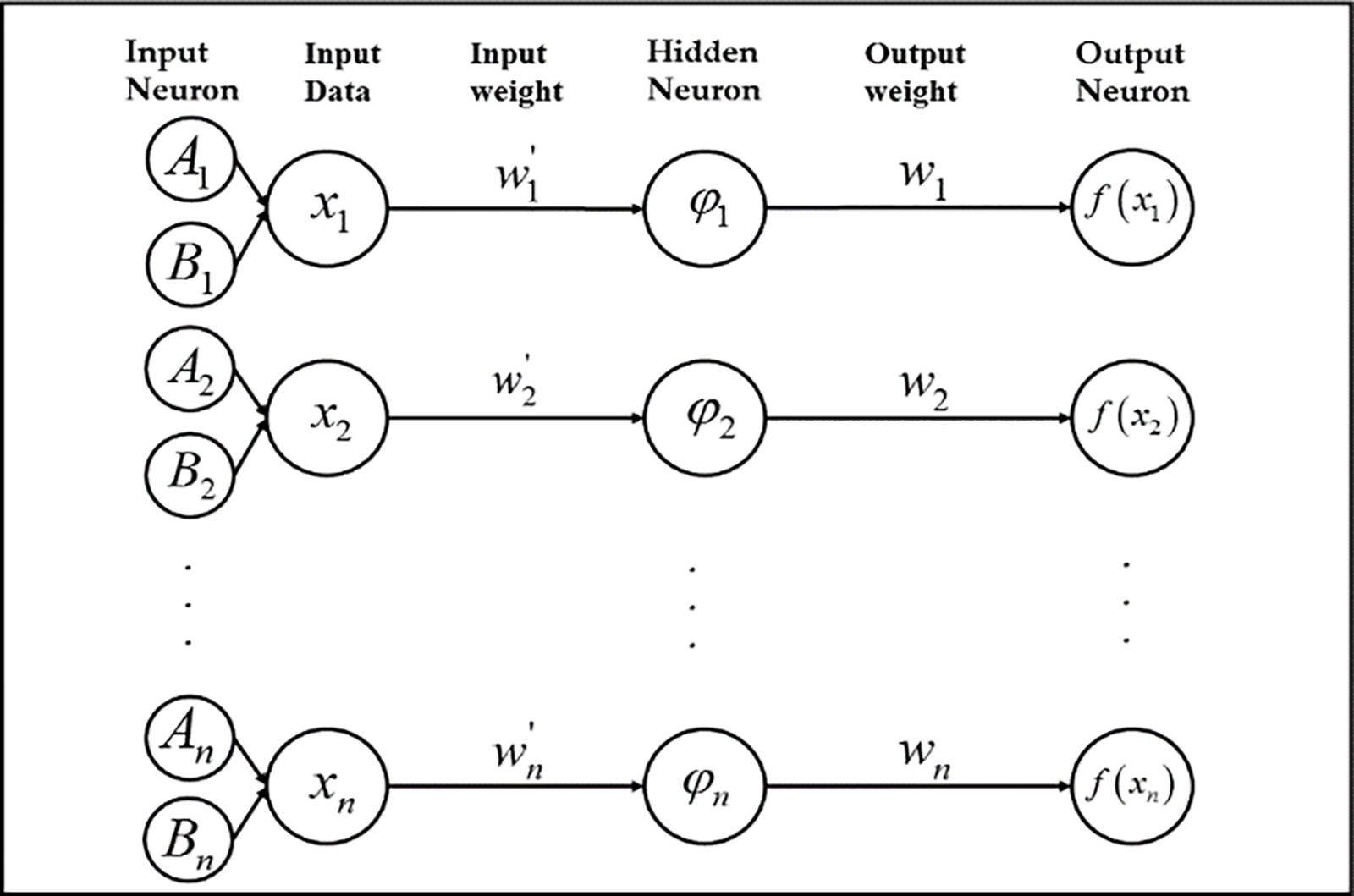
Figure 2: SRBFNN-2SAT structure

5  Genetic Algorithm (GA) in SRBFNN-2SAT

The GA represents a traditional metaheuristic algorithm utilized for solving multiple optimization problems. As for the GA structure, considering the finite solution space can be separated into two classifications: local search, in addition to global search [38]. Strings populations (also known as chromosomes) are solutions for many optimization problems in GA [39]. GA was used by Hamadneh et al. [2] for the specified centers of a hidden neuron width with a hidden neuron number by reducing the given absolute error sum of actual and required outputs. In the present study, GA has been utilized to improve SRBFNN-2SAT’s output weight by diminishing the error of the training. The GA application in SRBFNN is the SRBFNN-2SATGA. GA in RBFNN-2SATGA will calculate the output weight from the hidden layer to the output layer by employing the width and the center of the hidden neuron at the hidden layer. Thus, in SRBFNN, the network must detect an output weight by solving a given linear Eq. (9) comprising RBFNN output. GA, in this case, is used in the SRBFNN for improving the SRBFNN output weight solution. This solution (i.e., the output weight) in SRBFNN-2SAT produced by GA, represents a given chromosome. These chromosomes in GA will undergo mutation and crossover until the chromosome’s fitness is optimal (an error is diminished). Throughout this phase of crossover, a parent’s chromosome data is exchanged for producing further chromosomes with much higher fitness and a lower error. During the mutation phase, this chromosome data randomly changed only one value of output weight so that the solution is improved (i.e., the output weight) of the RBFNN. After that, GA will undergo 10000 iterations (i.e., Generations) to enhance chromosomes until the SRBFNN output is less or equivalent to the target logic programming output. These steps, which are involved in the SRBFNN-2SATGA, are presented in Fig. 3:

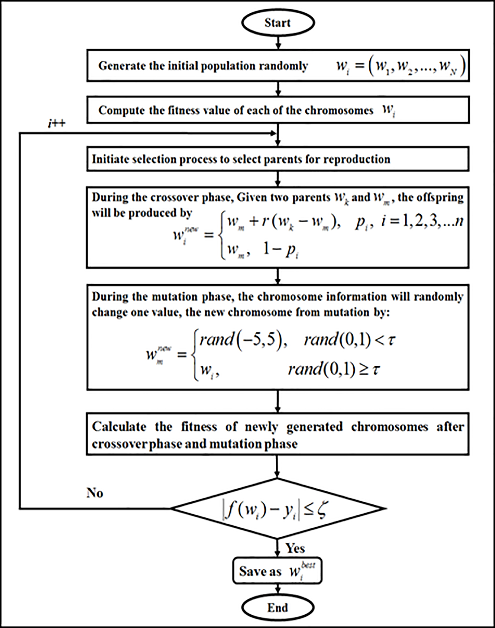
Figure 3: Flowchart of SRBFNN-2SATGA

6  Evolutionary Strategies Algorithm in SRBFNN-2SAT

Among other evolutionary algorithms, ES has been recently introduced [19]. ES draws upon adaptive selection principles that exist in the natural world [21]. These were successfully utilized to provide effective solutions for many optimization problems. Thus, each of the generations (i.e., the ES iteration) can take a specific population of the vectors (i.e., potential solutions) and modify the problem’s parameters to create offspring (i.e., innovative solutions) [20]. Parents and descendants are, thus, assessed. However, the highest appropriate vectors only (i.e., better solutions) can survive to produce a new generation. ES has successfully tackled a wide array of optimization problems [19]. In the present study, ES used for boosting SRBFNN-2SAT’s output weight via decreasing the training error; the ES in the SRBFNN-2SAT is referred to SRBFNN-2SATES. In SRBFNN-2SATES, ES will be computing an output weight by utilizing the hidden neuron’s center and width. Therefore, ES has been utilized in the SRBFNN-2SAT for improving the product or output weight solution. This solution, that is, the (i.e., the output weight) in this SRBFNN-2SAT produced by ES, represents a given population. These populations in ES will undergo recombination, mutation then selection until the population’s fitness is optimal (an error is diminished). Throughout this phase of recombination, population data is exchanged for producing other new populations with much higher fitness and a lower error. During the mutation phase, this population data randomly changed only one value of the output weight so that the solution improves the output weight wi of the SRBFNN-2SAT. ES will, therefore, be undertaking 10000 generations to enhance populations until the SRBFNN-2SAT output is less or equivalent to the target logic programming output. Fig. 4 shows the measures used in SRBFNN-2SATES:

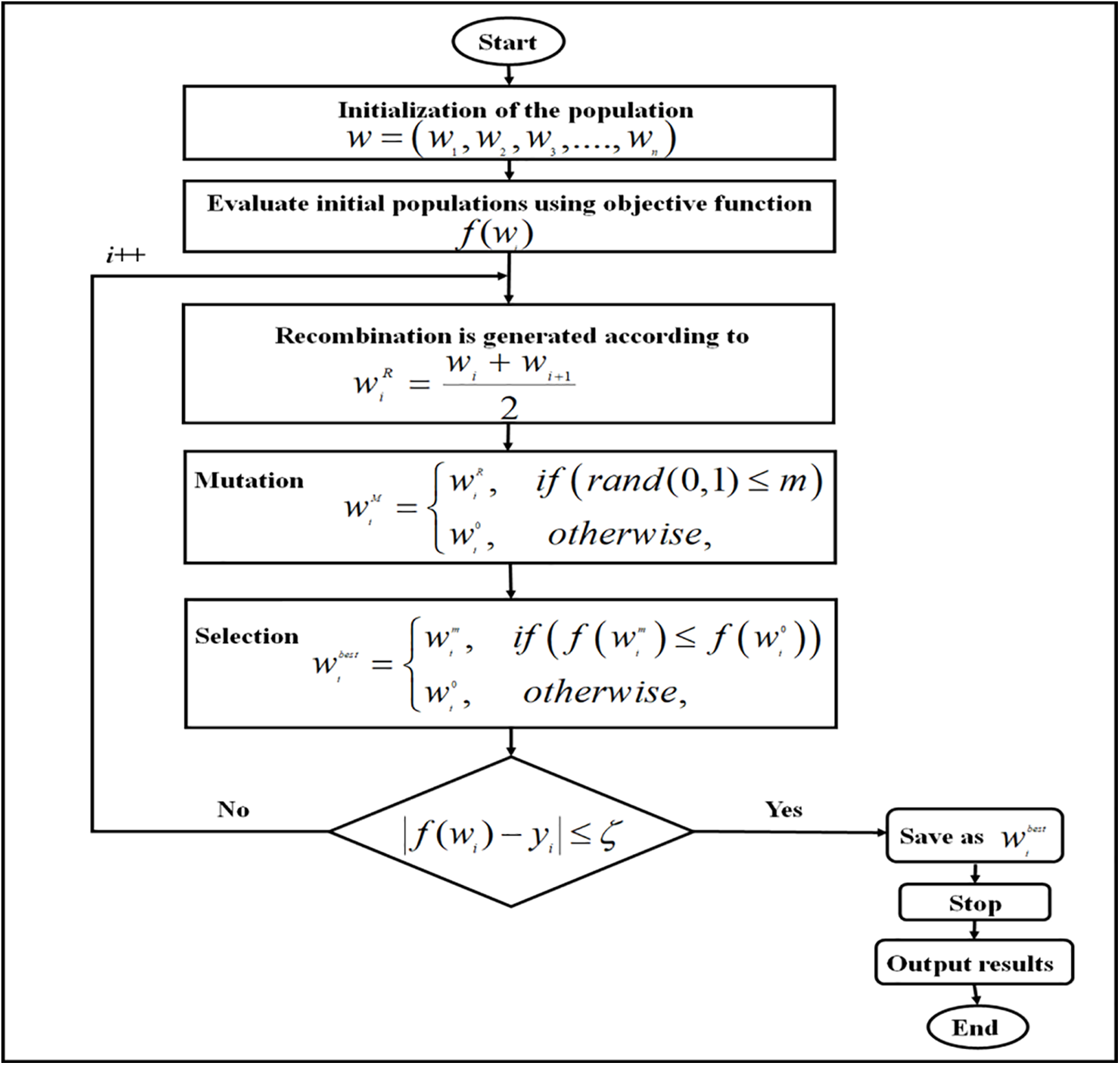
Figure 4: Flowchart of SRBFNN-2SATES

7  Differential Evolution Algorithm in SRBFNN-2SAT

The latest evolutionary population-based algorithm has been introduced by Storn et al. [14] (known as the DE algorithm), which is utilized in numerical optimization. The basic framework of the DE algorithm is classified into both local and global search using a flexible function optimizer [40]. GA and DE represent different algorithms. The main difference is that a DE’s selection operator possesses the relative probability for selection as parents. A chance is, therefore, independent of the solution’s fitness value. Each solution in DE competes with its parent, but the fittest wins [41]. DE signifies the method of population-based search using the nondeterministic polynomial (NP) variables as a population of the D dimensional parameter vectors for every generation. Therefore, the initial population has been selected indiscriminately if there is no information about the given problem. Hence, in terms of an initial solution, a specific initial population is produced by the addition of typically distributed arbitrary deviations for a given initial solution. The idea behind DE involves creating a new scheme to produce trial parameter vectors. Thus, DE produces innovative parameter vectors by combining a given weighted difference vector between two members of the population, as well as an extra third population member, and if the given vector achieved a smaller objective function value compared to the number of the encoded population, the generated vector substitutes the specific compared vector. Moreover, the superlative parameter vector can be assessed for each generation. Accordingly, any progress during the process of optimization can be tracked down. When the distance, and direction information, are extracted from the given population for producing random deviations, this will result in an adaptive scheme of outstanding properties of convergence [14,41]. Therefore, DE upholds a couple of arrays; each can hold a given population size (i.e., NP with D dimensional, using real-valued vectors). Therefore, the chief array holds the obtainable vector population, whereas the subordinate array accumulates the chosen vectors for a subsequent generation. Thus, in every generation, NP competitions are held for determining the subsequent generation composition. DE has been adopted in this work as a specific learning method throughout the training phase involves computing equivalent output weights, which connect the SRBFNN-2SAT hidden neurons and its output neurons. Accordingly, DE is utilized in the SRBFNN-2SAT to optimize the producer output weight solution in SRBFNN-2SAT, and this solution produced by DE represents a given population. These populations in DE will undergo an initial random selection of an initial parameter to verify if the fitness of the population is optimal or not. If not, the population undergo mutation, recombination, and selection until the population’s fitness is optimum (i.e., an error is diminished). Throughout this phase of mutation, population data is exchanged for producing other new populations with much higher fitness and a lower error. During the recombination, this population data randomly changed only one value of output weight so that the solution improves the output weight of the SRBFNN-2SAT. DE will subsequently undergo 10000 iterations to improve populations until the SRBFNN-2SAT output is less or equivalent to the target logic programming output. Fig. 5 shows the SRBFNN-2SATDE stages to improve connection weights amid a given hidden layer with a given output layer.

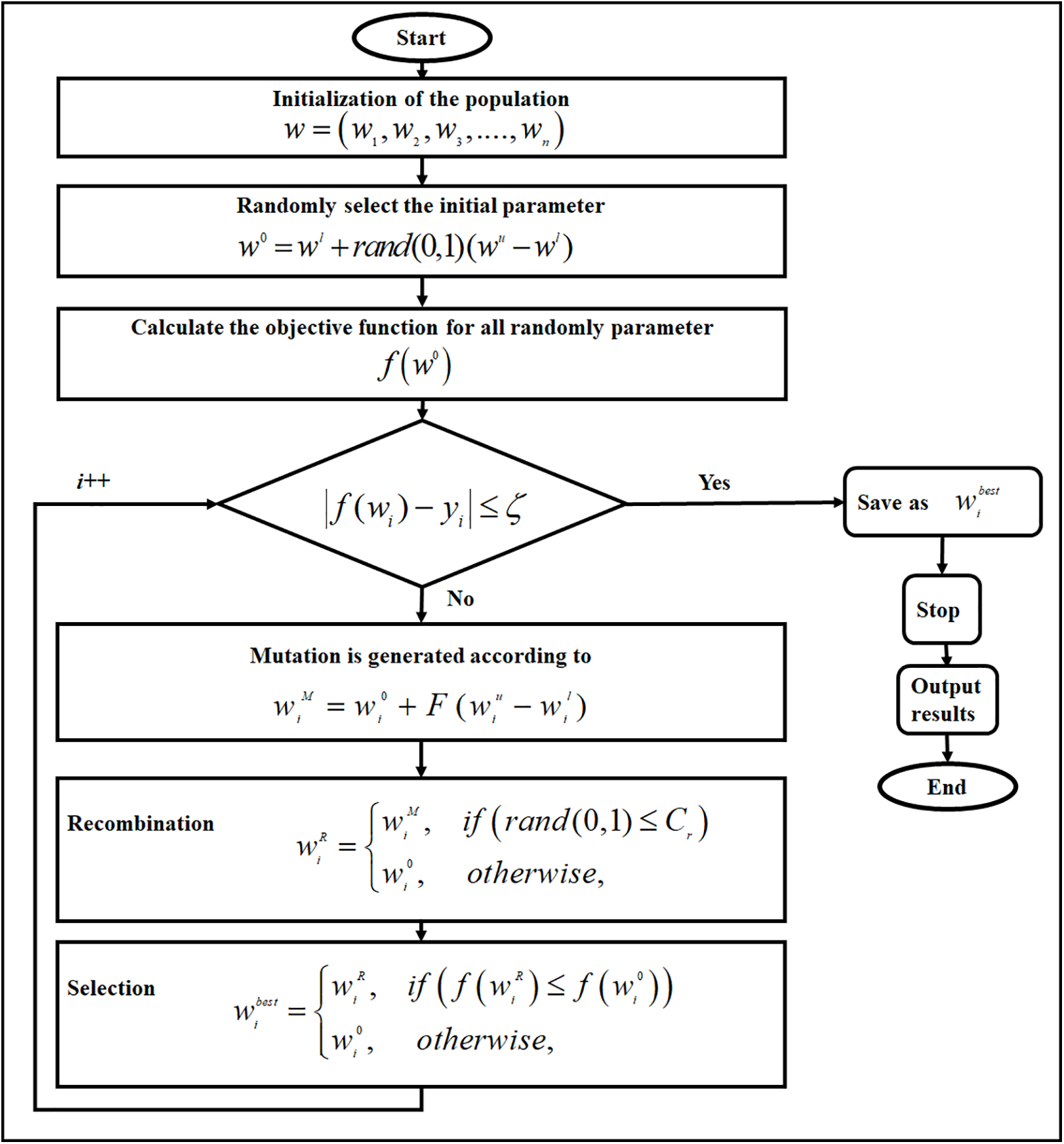
Figure 5: Flowchart of SRBFNN-2SATDE

8  Evolutionary Programming Algorithm in SRBFNN-2SAT

The EP algorithm was first observed by Lawrence J. Fogel in 1960 [15], a specified stochastic optimization approach resembling GA. However, instead of emphasizing the behavioral linkage among parents and descendants, it emulates natural genetic operators and, therefore, it represents the most optimal optimization technique due to these reasons:

1.    The EP algorithm can move from several points in the design space to another group of points. Therefore, EP functions more efficiently in finding the given global minima compared with the schemes, which operate by shifting from a certain point to another [25].

2.    The EP algorithm can utilize probabilistic transition rules, which is a critical advantage in acting as a model for highly exploitative searches [26].

3.    The EP algorithm is more capable of solving intricate engineering problems compared with other methods because it has a broader vector population, thereby providing the EP algorithm with multiple search spaces to minimize convergence prospects to a given non-global solution [15].

In the present work, EP was applied to boost the SRBFNN-2SAT network’s output weight so that the potential error of training is reduced. EP will randomly generate individuals to constitute the initial population to reduce the objective function. Then, the population of individuals will undergo a mutation process to generate a new individual via a random perturbation that generally distributes a one-dimensional random number with a mean of zero and a standard deviation of one for each component of the given individuals and throughout the process of selection, when the trial vector is equivalent or lower than the objective function vs. a target vector, it can be substituted in the subsequent generation; otherwise, this targeting vector retains the position in the given population for a different generation—the EP iterates up to a total of 10000 generations. When the condition of the solution termination is fulfilled, the algorithm's calculation is terminated. Thus, the SRBFNN-2SAT’s final output is the ideal SRBFNN-2SATEP output weight. EP in SRBFNN-2SAT becomes SRBFNN-2SATEP. Thus, in SRBFNN-2SATEP, EP determines an output weight applying center-width in a hidden neuron. Fig. 6 shows the stages followed in SRBFNN-2SATEP.

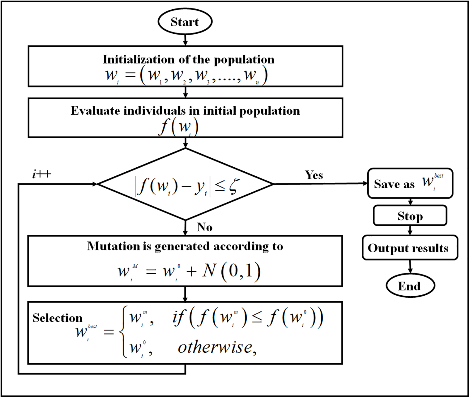
Figure 6: Flowchart of SRBFNN-2SATEP

Evolutionary Programming Algorithm (EP) with Symbolic Radial Basis Function Neural Network (RBFNN-2SAT) can be used in various scientific [42], engineering fields, epidemic models [43–45] or dam crack modeling [46], and can used it at mathematical models [47,48].

9  Results and Discussion

The entire suggested SRBFNN-2SAT paradigms were applied in Microsoft Visual Dev C++ software in Microsoft Windows 7, 64-bit, hard drive specification of 500 GB, RAM of 4096 MB, and a processor of 3.40 GHz. The computer-generated data sets (Simulated data) [49,50] have been generated through random input data. This selection of data diminished any bias and covered a more exhaustive search space and the (NN), i.e., the input neurons number differs between NN = 6, and NN = 120. The produced data considered specific binary values using a given structure based on the number of the clause, and generated data were applied for verifying how the introduced models perform in classifying the state of the neuron into an optimal or suboptimal state. Hamadneh et al. [49] and Sathasivam et al. [50] created these data in SAT logic using ANN. The final output of these models was converted to a binary representation ahead of the assessment of their error performance using Eq. (10) [37].

(S1RBFNN−2SAT,…,SNRBFNN−2SAT)={1,rand(0,1)<0.50,otherwise(10)

whereby true-false states corresponded 1 through 0 for final output of these models after converted to a binary representation. Thereby, based on the SRBFNN-2SAT model’s simulations, the 2SAT training phase’s quality was assessed through various performance metrics, involving Mean Absolute Relative Error (MARE), Root Mean Square Error (RMSE), Mean Absolute Percentage Error (MAPE), Mean Bias Error (MBE), Systematic Error (SD), Schwarz Bayesian Criterion (SBC), in addition to CPU Time. Thus, each of the performance metrics equation is presented as follows [3,8,51] whereby:

Mean Absolute Relative Error (MARE):

MARE=∑i=1n1n|f(wi)−yi||f(wi)|(11)

Root Mean Square Error (RMSE):

RMSE=∑i=1n1n(f(wi)−yi)2(12)

Mean Absolute Percentage Error (MAPE):

MAPE=100%n∑i=1n|(f(wi)−yi)yi|(13)

Mean Bias Error (MBE):

MBE=1n∑i=1n(f(wi)−yi)(14)

Systematic Error (SD):

SD=∑i=1nRMSE2−MBE2(15)

Schwarz Bayesian Criterion (SBC) [49]:

SBC=nln⁡(∑i=1n(f(wi)−yi)2n)+paln⁡(n)(16)

wherein f(wi) refers to the value of the producer output of SRBFNN-2SAT, yi indicates the target logic programming output value, and n signifies the target data number. The computation time will be considered for evaluating the SRBFNN-2SAT model’s efficiency. In contrast, CPU time indicates the necessary period of models of SRBFNN-2SAT so, that a single execution is completed, involving SRBFNN-2SAT models’ capability, as well as stability. CPU Time to evaluate SRBFNN models will be in the following equation:

CPUtime=TrainingTime+TestingTime(17)

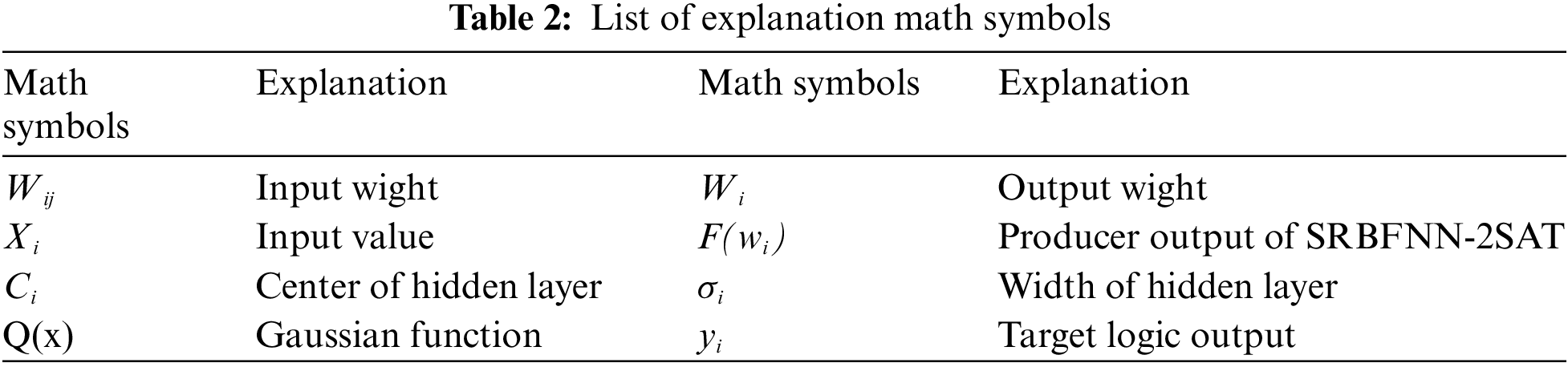
The following Table 2 to explains all math symbols that used at this study.

The results of the four different EAs to train SRBFNN-2SAT constructed by the logic programming 2SAT called SRBFNN-2SATGA, SRBFNN-2SATES, SRBFNN-2SATDE, along with SRBFNN-2SATEP are encapsulated into Figs. 7 to 13. These four algorithms are popular in searching for a given near-optimal solution for SRBFNN-2SAT. Nonetheless, no efforts were directed to identify the impact of EAs to train RBFNN based on logic programming 2SAT. The current work only involves the four different EAs, GA, ES, DE, and EP that contribute to enhancing the structure of SRBFNN-2SAT. Experimentally speaking, the most optimum model is the SRBFNN-2SATEP because it obtained the improved weight via linking a hidden layer in RBFNN to an output layer by 2SAT logical rule with minimum values for MARE, RMSE, MAPE, MBE, SD, SBC, and CPU time. The model of SRBFNN-2SATEP demonstrated the most optimum performance concerning the errors as this neuron number has been enhanced, as per Figs. 7 to 13. EP outperformed several existing algorithms’ effectiveness, as well as their convergence speed, because of this model’s numerous features involving robustness, flexibility, and random competition.

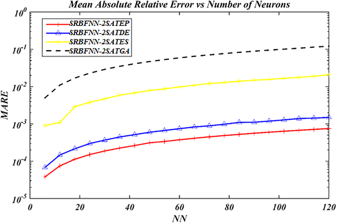
Figure 7: MARE value for all SRBFNN-2SAT models

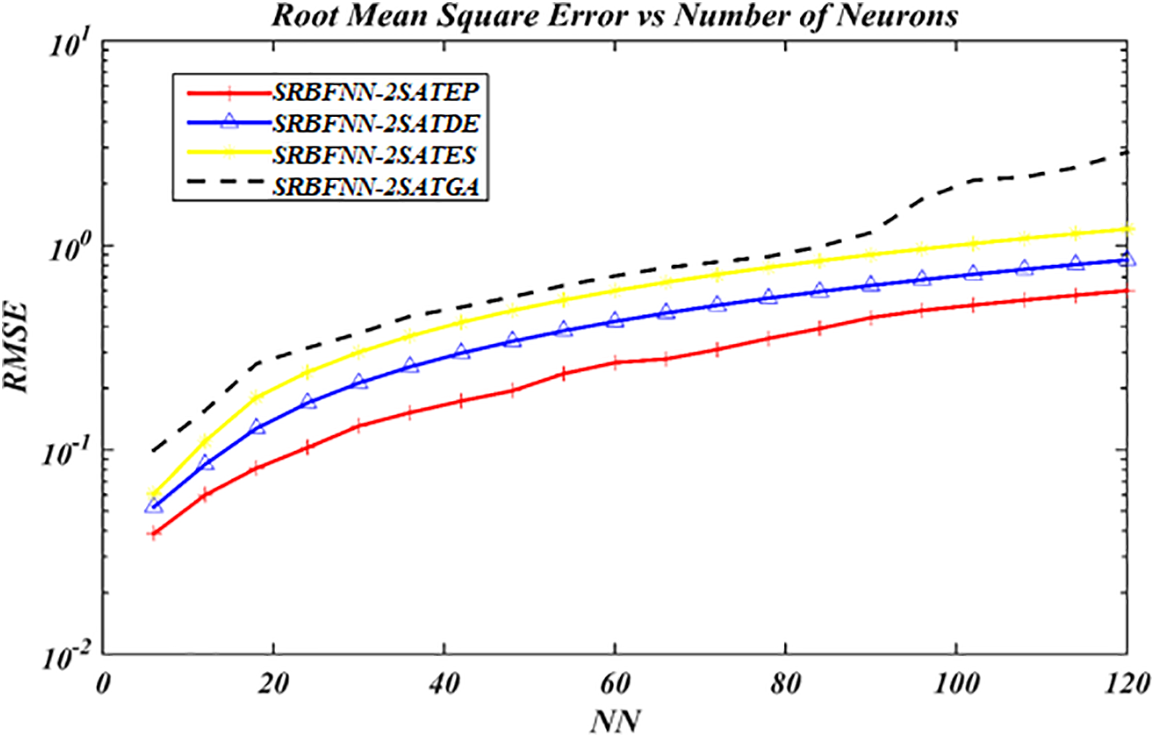
Figure 8: RMSE value for the complete SRBFNN-2SAT models

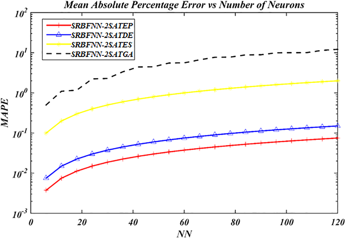
Figure 9: MAPE value for the complete SRBFNN-2SAT models

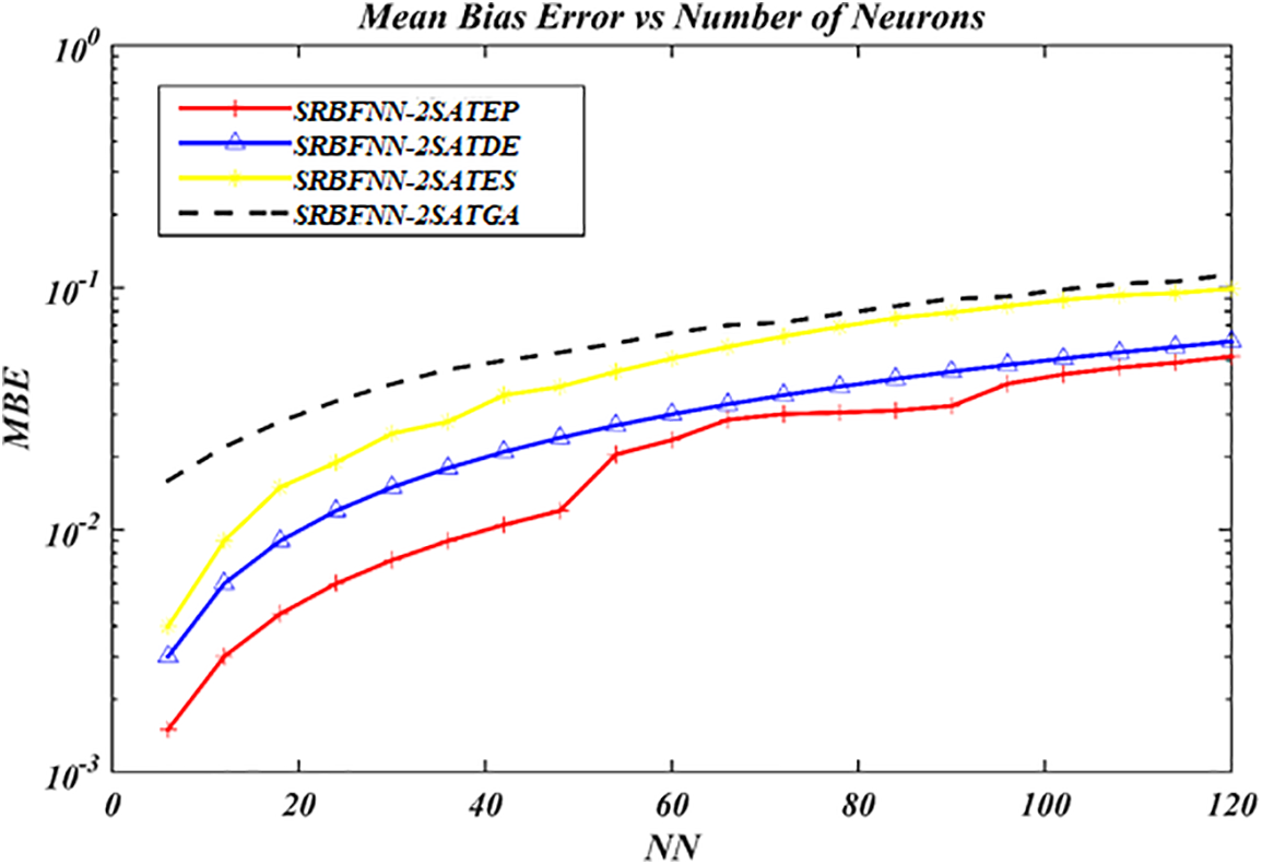
Figure 10: MBE value for the complete SRBFNN-2SAT models

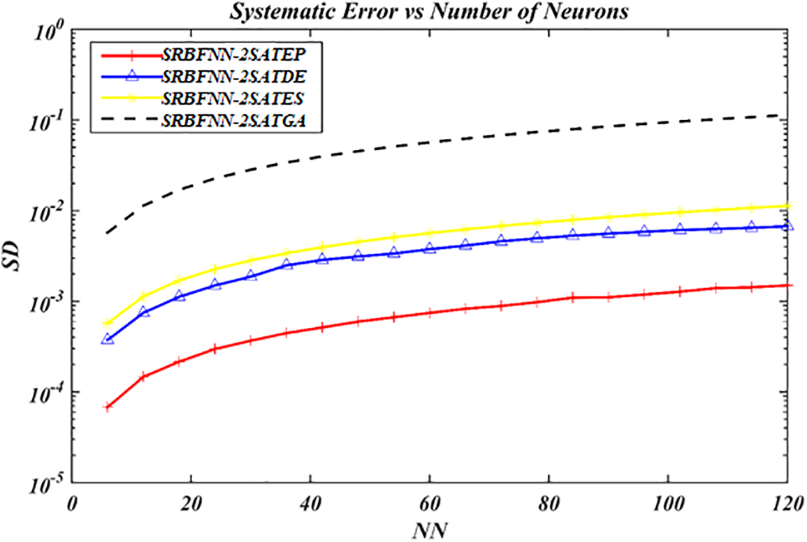
Figure 11: SD Evaluation for the complete SRBFNN-2SAT models

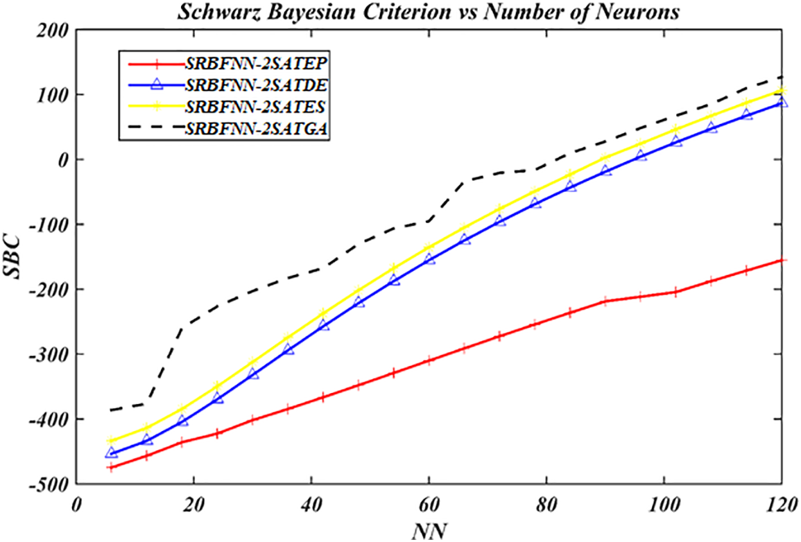
Figure 12: SBC value for the complete SRBFNN-2SAT models

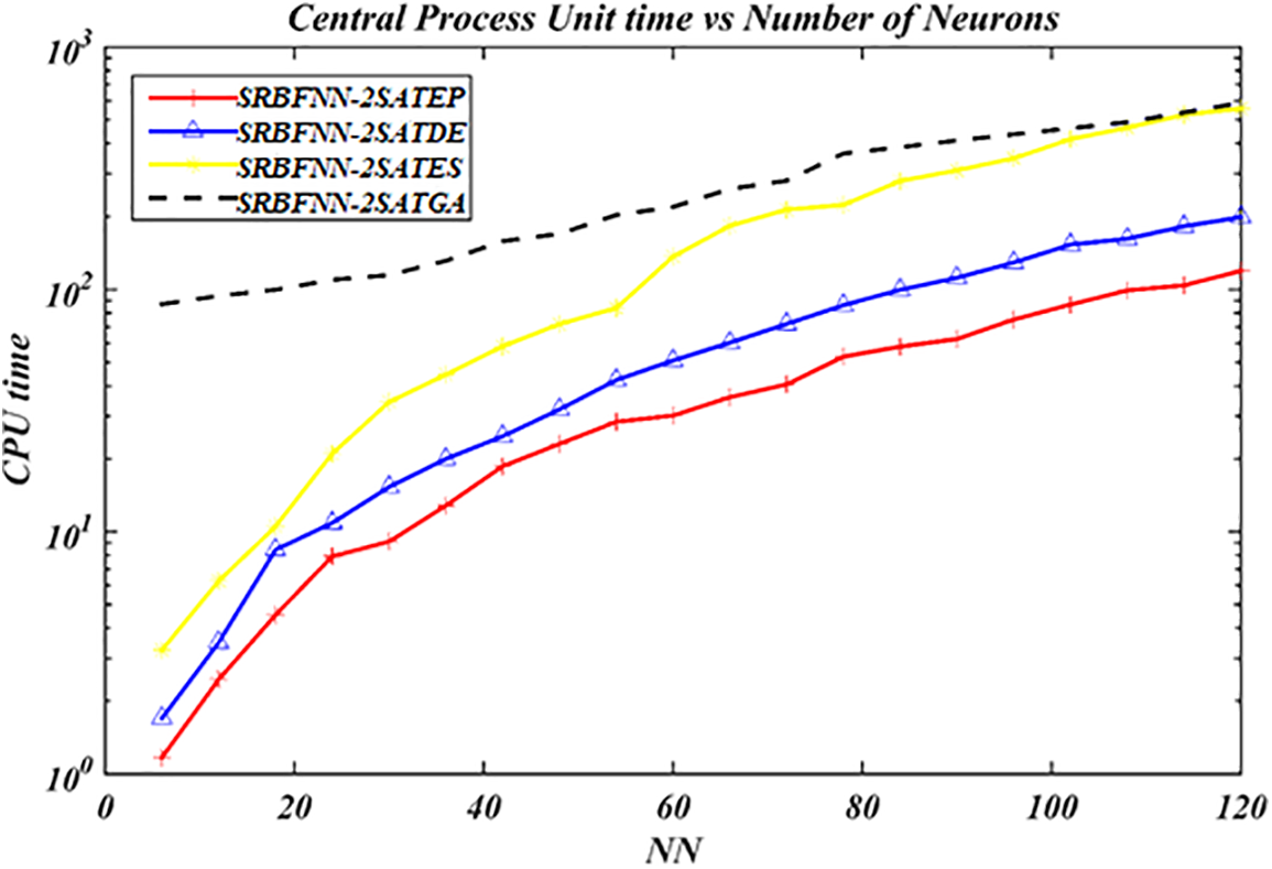
Figure 13: The CPU time value for the complete SRBFNN-2SAT models

As observed in Fig. 7, SRBFNN-2SATEP achieved a low MARE value compared to these models: SRBFNN-2SATDE, SRBFNN-2SATES, with the SRBFNN-2SATRAGA. MARE exemplifies a practical error estimator tool, among other tools. The MARE result demonstrated that EP had outperformed efficiently compared with other algorithms of good solutions with less error. This because the operators in EP are the instrumental factors contributing to the algorithm's speed.

Fig. 8 demonstrates RMSE performance in training SRBFNN-2SATEP and SRBFNN-2SATDE, with SRBFNN-2SATES, as well as SRBFNN-2SATGA. Consequently, using this approach of SRBFNN-2SATEP was comparatively more efficient compared with SRBFNN-2SATDE and SRBFNN-2SATES, as well as SRBFNN-2SATGA because there exist effective EP operators like a mutation with a typical distribution of one-dimensional randomly selected number using mean zero and standard deviation. The normal distribution indicates that the utilized random number has produced a new number for each of the population value in the training phase, which improved the solutions’ quality.

Based on the MAPE, as shown in Fig. 9, SRBFNN-2SATEP reliably achieved MAPE with a less value than the whole number of the given neurons. Nonetheless, MAPE for SRBFNN-2SATDE, SRBFNN-2SATES, and SRBFNN-2SATGA significantly increased until the last simulations. With a lower MAPE value, profound evidence was provided about the efficient EP performance with the SRBFNN-2SAT. Those optimization operators as a mutation in the SRBFNN-2SATEP model achieved the ultimate outputs, minimizing the suboptimal state percentage compared with SRBFNN-2SATDE, SRBFNN-2SATES, and SRBFNN-2SATGA.

In Fig. 10, similar results were obtained for the values of MBE vs. the values of SRBFNN-2SATEP, SRBFNN-2SATDE, SRBFNN-2SATES, and SRBFNN-2SATGA. MBE signifies the actual error, and it has been widely applied by scholars to examine the solution’s accuracy for models. As observed in Fig. 10, SRBFNN-2SATEP had a more robust capability of training the SRBFNN according to the logic programming 2SAT vs. these models: SRBFNN-2SATDE, SRBFNN-2SATES, and SRBFNN-2SATGA due to MBE lower values.

As shown in Fig. 11, the SD Error performance is displayed in training the SRBFNN-2SAT models. Regarding SD, it can be defined as an accuracy tool used for determining the algorithm’s ability to train the network [49] and lower values of SD mean better algorithm accuracy. SRBFNN-2SATEP revealed the ideal performance concerning SD even though this neuron’s number has increased, as observed in Fig. 11. However, the SBC smallest value revealed that this model represents the most optimum model [49].

Fig. 12 indicates that EP in SRBFNN-2SATEP proved the ideal performance concerning SBC even though the number of these neurons increased. Regarding CPU time, the EP performance in SRBFNN-2SATEP was faster than other existing algorithms (refer to Fig. 13). Thus, in the NN > 15, the opportunity for SRBFNN-2SATGA and SRBFNN-2SATES to be trapped in this trial/error state increased, which made GA achieve premature convergence. Nevertheless, SRBFNN-2SATGA enjoys an exceptional learning error, which can be attributed to the unsuccessful initial crossover and, therefore, some iterations were essential for the utilized SRBFNN-2SATGA so that the output weight is generated, which is higher in quality, among other attributes, during which, a mutation signifies one active operator only. The problem was worse if the given suboptimal output weight among these attributes required a floating number.

In this study, the findings substantiated that EP has the capability of effectively alleviating the current algorithms’ drawbacks when training SRBFNN-2SAT in the MARE, RMSE, MAPE, MBE, SD, SBC, and CPU time. The findings established that there has been a significant model improvement of SRBFNN via applying EP to perform logic programming 2SAT in assisting the ideal logical rule to govern the network’s behavior. The discussion and analysis results validated that EP demonstrated a faster rate of convergence, providing superior results, whereas EP demonstrated lower values for MARE, RMSE, MAPE, MBE, SD error, and SBC, accompanied by faster CPU time for training the SRBFNN-2SAT model. EP has, therefore, exhibited efficient performance in training the SRBFNN-2SAT. Based on NFL, i.e., (No Free Lunch theorem), no algorithm has ever been able to perform better than every other algorithm in every optimization problem [52]. This means there is a potential limitation of the study related to time series problems or continuous problems.

10  Conclusion and Future Work

Inspired by the population-based heuristic global optimization technique, which is characterized by being easy to digest, simple in implementation, fast, and reliable, a specific hybrid paradigm has been proposed in this paper. Different EAs with SRBFNN-2SAT have been integrated so that logic programming 2SAT can be executed. These suggested algorithms included the GA algorithm, the ES algorithm, and the DE algorithm, in addition to the EP algorithm. The findings showed enormous variations in how these four paradigms performed regarding MARE, RMSE, MAPE, MBE, SD Error, SBC, and CPU time. Moreover, the experimental results showed that the SRBFNN-2SATEP paradigm provided a small error value of MARE, RMSE, MAPE, MBE, SD, SBC, and much quicker computation time in comparison with SRBFNN-2SATGA, SRBFNN-2SATES, and RBF-2SATDE. The EP algorithm has, therefore, been more robust in comparison with GA, ES, and DE in certain aspects, including much lower error, together with quicker process time to execute the 2SAT logic programming in RBFNN. In Future work, SRBFNN-2SATEP can be extended in further studies to Satisfiability logics like MIN-SAT and MAX-SAT, as well as various SAT logics. Therefore, it is highly potential that the application of the SRBFNN-2SATEP model can be effectively utilized in real-life data sets.

Acknowledgement: This work is supported by Ministry of Higher Education (MOHE) through Fundamental Research Grant Scheme (FRGS) (FRGS/1/2020/STG06/UTHM/03/7).

Funding Statement: This research is funded by Fundamental Research Grant Scheme, No. FRGS/1/20 20/STG06/UTHM/03/7 by the Ministry of Higher Education, Malaysia and registrar of Universisti Tun Hussein Onn Malaysia.

Conflicts of Interest: The authors declare that they have no conflicts of interest to report regarding the present study.

References

1. H. de Leon-Delgado, R. J. Praga-Alejo, D. S. Gonzalez-Gonzalez and M. Cantú-Sifuentes, “Multivariate statistical inference in a radial basis function neural network,” Expert Systems with Applications, vol. 93, pp. 313–321, 2018. [Google Scholar]

2. N. Hamadneh, S. Sathasivam, S. L. Tilahun and O. H. Choon, “Learning logic programming in radial basis function network via genetic algorithm,” Journal of Applied Sciences (Faisalabad), vol. 12, no. 9, pp. 840–847, 2012. [Google Scholar]

3. S. Alzaeemi, M. A. Mansor, M. S. M. Kasihmuddin, S. Sathasivam and M. Mamat, “Radial basis function neural network for two satisfiability programming,” Indonesian Journal of Electrical Engineering and Computer Science, vol. 18, no. 1, pp. 459–469, 2020. [Google Scholar]

4. Y. Ge, J. Li, W. Jiang, L. Wang and S. Duan, “A spintronic memristive circuit on the optimized RBF-MLP neural network,” Chinese Physics B, vol. 31, no. 11, pp. 110702, 2022. [Google Scholar]

5. J. Yang and J. Ma, “Feed-forward neural network training using sparse representation,” Expert Systems with Applications, vol. 116, pp. 255–264, 2019. [Google Scholar]

6. M. S. M. Kasihmuddin, M. A. Mansor, M. B. M. Faisal and S. Sathasivam, “Discrete mutation hopfield neural network in propositional satisfiability,” Mathematics, vol. 7, no. 11, pp. 1133–1154, 2019. [Google Scholar]

7. M. S. M. Kasihmuddin, M. A. Mansor and S. Sathasivam, “Discrete hopfield neural network in restricted maximum k-satisfiability logic programming,” Sains Malaysiana, vol. 47, no. 6, pp. 1327–1335, 2018. [Google Scholar]

8. M. S. M. Kasihmuddin, M. A. Mansor, S. A. Alzaeemi and S. Sathasivam, “Satisfiability logic analysis via radial basis function neural network with artificial bee colony algorithm,” International Journal of Interactive Multimedia and Artificial Intelligence, vol. 6, no. 6, pp. 164–174, 2021. [Google Scholar]

9. N. Hamadneh, S. Sathasivam and O. H. Choon, “Higher order logic programming in radial basis function neural network,” Applied Mathematical Sciences, vol. 6, no. 3, pp. 115–127, 2012. [Google Scholar]

10. F. Rezaei, S. Jafari, A. Hemmati-Sarapardeh and A. H. Mohammadi, “Modeling of gas viscosity at high pressure-high temperature conditions: Integrating radial basis function neural network with evolutionary algorithms,” Journal of Petroleum Science and Engineering, vol. 208, pp. 109328, 2022. [Google Scholar]

11. R. D. Dandagwhal and V. D. Kalyankar, “Design optimization of rolling element bearings using advanced optimization technique,” Arabian Journal for Science and Engineering, vol. 44, no. 9, pp. 7407–7422, 2019. [Google Scholar]

12. J. H. Holland, “Genetic algorithms and the optimal allocation of trials,” SIAM Journal on Computing, vol. 2, no. 2, pp. 88–105, 1973. [Google Scholar]

13. I. Rechenberg, “Evolution strategy: Optimization of technical systems by means of biological evolution,” Fromman-Holzboog, Stuttgart, vol. 104, pp. 15–16, 1973. [Google Scholar]

14. R. Storn and K. Price, “Differential evolution is a simple and efficient heuristic for global optimization over continuous spaces,” Journal of Global Optimization, vol. 11, no. 4, pp. 341–359, 1997. [Google Scholar]

15. L. J. Fogel, A. J. Owens and M. J. Walsh, Artificial Intelligence through Simulated Evolution. New York-London-Sydney: John Wiley and Sons, Inc. XII, pp. 170, 1966. [Google Scholar]

16. D. E. Goldberg and J. H. Holland, “Genetic algorithms and machine learning,” Machine Learning, vol. 2, no. 3, pp. 95–99, 1988. [Google Scholar]

17. M. Pandey, M. Zakwan, P. K. Sharma and Z. Ahmad, “Multiple linear regression and genetic algorithm approach to predict temporal scour depth near the circular pier in non-cohesive sediment,” ISH Journal of Hydraulic Engineering, vol. 26, no. 1, pp. 96–103, 2020. [Google Scholar]

18. Z. Jing, J. Chen and X. Li, “RBF-GA: An adaptive radial basis function metamodeling with genetic algorithm for structural reliability analysis,” Reliability Engineering & System Safety, vol. 189, pp. 42–57, 2019. [Google Scholar]

19. N. Moreira, T. Miranda, M. Pinheiro, P. Fernandes, D. Dias et al., “Back analysis of geomechanical parameters in underground works using an evolution strategy algorithm,” Tunnelling and Underground Space Technology, vol. 33, pp. 143–158, 2013. [Google Scholar]

20. F. E. Fernandes Jr. and G. G. Yen, “Pruning of generative adversarial neural networks for medical imaging diagnostics with evolution strategy,” Information Sciences, vol. 558, pp. 91–102, 2021. [Google Scholar]

21. K. Karabulut, H. Öztop, L. Kandiller and M. F. Tasgetiren, “Modeling and optimization of multiple traveling Salesmen problems: An evolution strategy approach,” Computers & Operations Research, vol. 129, pp. 105192, 2021. [Google Scholar]

22. D. Deepika and N. Balaji, “Effective heart disease prediction with greywolf with firefly algorithm-differential evolution (GF-DE) for feature selection and weighted ANN classification,” Computer Methods in Biomechanics and Biomedical Engineering, vol. 25, no. 12, pp. 1409–1427, 2022. [Google Scholar] [PubMed]

23. Y. Xue, Y. Tong and F. Neri, “An ensemble of differential evolution and Adam for training feed-forward neural networks,” Information Sciences, vol. 608, pp. 453–471, 2022. [Google Scholar]

24. W. Tao, J. Chen, Y. Gui and P. Kong, “Coking energy consumption radial basis function prediction model improved by differential evolution algorithm,” Measurement and Control, vol. 52, no. 8, pp. 1122–1130, 2019. [Google Scholar]

25. N. J. Singh, S. Singh, V. Chopra, M. A. Aftab, S. M. Hussain et al., “Chaotic evolutionary programming for an engineering optimization problem,” Applied Sciences, vol. 11, no. 6, pp. 2717, 2021. [Google Scholar]

26. H. Tian, S. C. Chen and M. L. Shyu, “Evolutionary programming-based deep learning feature selection and network construction for visual data classification,” Information Systems Frontiers, vol. 22, no. 5, pp. 1053–1066, 2020. [Google Scholar]

27. H. Naseri, M. Ehsani, A. Golroo and F. Moghadas Nejad, “Sustainable pavement maintenance and rehabilitation planning using differential evolutionary programming and coyote optimization algorithm,” International Journal of Pavement Engineering, vol. 23, no. 8, pp. 2870–2887, 2021. [Google Scholar]

28. Y. J. Gong, W. N. Chen, Z. H. Zhan, J. Zhang, Y. Li et al., “Distributed evolutionary algorithms and their models: A survey of the state-of-the-art,” Applied Soft Computing, vol. 34, pp. 286–300, 2015. [Google Scholar]

29. C. D. James and S. Mondal, “Optimization of decoupling point position using metaheuristic evolutionary algorithms for smart mass customization manufacturing,” Neural Computing and Applications, vol. 33, no. 17, pp. 11125–11155, 2021. [Google Scholar] [PubMed]

30. R. E. M. Bastos, M. C. Goldbarg, E. F. G. Goldbarg and M. da Silva Menezes, “Evolutionary algorithms for the traveling salesman with multiple passengers and high occupancy problem,” in 2020 IEEE Congress on Evolutionary Computation (CEC), Glasgow, UK, vol. 1, pp. 1–8, 2020. [Google Scholar]

31. J. Moody and C. J. Darken, “Fast learning in networks of locally-tuned processing units,” Neural Computation, vol. 1, no. 2, pp. 281–294, 1989. [Google Scholar]

32. D. Lowe, “Adaptive radial basis function nonlinearities, and the problem of generalization,” in Artificial Neural Networks, First IEE Int. Conf., 16–18 October, London, UK, vol. 1, pp. 171–175, 1989. [Google Scholar]

33. A. K. Hassan, M. Moinuddin, U. M. Al-Saggaf and M. S. Shaikh, “On the kernel optimization of radial basis function using nelder mead simplex,” Arabian Journal for Science and Engineering, vol. 43, no. 6, pp. 2805–2816, 2018. [Google Scholar]

34. M. A. Hossain and M. Shahjahan, “Memoryless radial basis function neural network based proportional integral controller for PMSM drives,” International Journal of Power Electronics and Drive Systems, vol. 14, no. 1, pp. 89, 2023. [Google Scholar]

35. S. A. S. Alzaeemi and S. Sathasivam, “Examining the forecasting movement of palm oil price using RBFNN-2SATRA metaheuristic algorithms for logic mining,” IEEE Access, vol. 9, pp. 22542–22557, 2021. [Google Scholar]

36. L. Shang, H. Nguyen, X. N. Bui, T. H. Vu, R. Costache et al., “Toward state-of-the-art techniques in predicting and controlling slope stability in open-pit mines based on limit equilibrium analysis, radial basis function neural network, and brainstorm optimization,” Acta Geotechnica, vol. 17, no. 4, pp. 1295–1314, 2022. [Google Scholar]

37. J. Chen, M. S. M. Kasihmuddin, Y. Gao, Y. Guo, M. A. Mansor et al., “PRO2SAT: Systematic probabilistic satisfiability logic in discrete hopfield neural network,” Advances in Engineering Software, vol. 175, pp. 103355, 2023. [Google Scholar]

38. Y. Liu, C. Jiang, C. Lu, Z. Wang and W. Che, “Increasing the accuracy of soil nutrient prediction by improving genetic algorithm backpropagation neural networks,” Symmetry, vol. 15, no. 1, pp. 151, 2023. [Google Scholar]

39. H. Marouani, K. Hergli, H. Dhahri and Y. Fouad, “Implementation and identification of preisach parameters: Comparison between genetic algorithm, particle swarm optimization, and levenberg-marquardt algorithm,” Arabian Journal for Science and Engineering, vol. 44, no. 8, pp. 6941–6949, 2019. [Google Scholar]

40. S. L. Wang, F. Ng, T. F. Morsidi, H. Budiman and S. C. Neoh, “Insights into the effects of control parameters and mutation strategy on self-adaptive ensemble-based differential evolution,” Information Sciences, vol. 514, no. 3, pp. 203–233, 2020. [Google Scholar]

41. K. R. Opara and J. Arabas, “Differential evolution: A survey of theoretical analyses,” Swarm and Evolutionary Computation, vol. 44, pp. 546–558, 2019. [Google Scholar]

42. M. Turkyilmazoglu, “Explicit formulae for the peak time of an epidemic from the SIR model,” Physica D: Nonlinear Phenomena, vol. 422, pp. 132902, 2021. [Google Scholar] [PubMed]

43. M. Turkyilmazoglu, “An extended epidemic model with vaccination: Weak-immune SIRVI,” Physica A: Statistical Mechanics and its Applications, vol. 598, pp. 127429, 2022. [Google Scholar] [PubMed]

44. M. Turkyilmazoglu, “A restricted epidemic SIR model with elementary solutions,” Physica A: Statistical Mechanics and its Applications, vol. 600, pp. 127570, 2022. [Google Scholar]

45. A. Raza, M. Rafiq, J. Awrejcewicz, N. Ahmed, M. Mohsin et al., “Dynamical analysis of coronavirus disease with crowding effect, and vaccination: A study of third strain,” Nonlinear Dynamics, vol. 107, no. 4, pp. 3963–3982, 2022. [Google Scholar] [PubMed]

46. J. Wang, Y. Zou, P. Lei, R. S. Sherratt and L. Wang, “Research on recurrent neural network based crack opening prediction of concrete dam,” Journal of Internet Technology, vol. 21, no. 4, pp. 1151–1160, 2020. [Google Scholar]

47. A. E. Abouelregal and M. Marin, “The response of nanobeams with temperature-dependent properties using state-space method via modified couple stress theory,” Symmetry, vol. 12, no. 8, pp. 1276, 2020. [Google Scholar]

48. M. L. Scutaru, S. Vlase, M. Marin and A. Modrea, “New analytical method based on dynamic response of planar mechanical elastic systems,” Boundary Value Problems, vol. 2020, no. 1, pp. 1–16, 2020. [Google Scholar]

49. N. Hamadneh, S. Sathasivam, S. L. Tilahun and O. H. Choon, “Satisfiability of logic programming based on radial basis function neural networks,” in AIP Conf. Proc., Penang, Malaysia, AIP, vol. 1605, pp. 547–550, 2014. https://doi.org/10.1063/1.5041551 [Google Scholar] [CrossRef]

50. S. Sathasivam, M. Mansor, M. S. M. Kasihmuddin and H. Abubakar, “An election algorithm for random k satisfiability in the Hopfield neural network,” Processes, vol. 8, no. 5, pp. 568, 2020. [Google Scholar]

51. T. Kato, “Prediction of photovoltaic power generation output and network operation,” In: Integration of Distributed Energy Resources in Power Systems, London, UK: Academic Press, pp. 77–108, 2016. [Google Scholar]

52. Y. C. Ho and D. L. Pepyne, “Simple explanation of the no free lunch theorem of optimization,” Cybernetics and Systems Analysis, vol. 38, no. 2, pp. 292–298, 2002. [Google Scholar]