Network Security Situation Prediction Based on TCAN-BiGRU Optimized by SSA and IQPSO

1  Introduction

As the network environment gets increasingly complicated, network security [1] has been a critical national concern in the current era. Tasks related to network security situation prediction (NSSP) have appeared accordingly. Predicting the future security situation of the network can guide network defense to reduce the adverse impact of network attacks. The commonly used methods of NSSP include gray theory [2], Markov Chain [3,4], evidence theory [5,6], and neural networks.

The traditional methods for situation prediction are time-series analysis, gray theory, etc. Time-Series Analysis is a method that arranges situational data from different periods according to their chronological order. It can fully explore the potential interdependence law between the situation data and use it to establish a dynamic model to achieve real-time monitoring and prediction of the situation data. This method is a quantitative prediction, and the principle is relatively simple. Suppose the situation has some potential connection with the previous times. In that case, the situation in the past N periods can be used to predict the situation in the following period. Commonly used models are Moving average (MA), Auto-Regressive (AR), and hybrid models. Li et al. [7] used the hidden Markov model to fully explore and analyze the interdependence of network posture before and after multiple heterogeneous data sources. Then they fused the security posture of all hosts in the network to quantify the security posture in the following period. Yang et al. [8] combined the least squares support vector machine, autoregressive model (AR), and RBF network to form a prediction model of information fusion and experimentally verified that the model outperformed a single prediction model. Scholars favor the Grey Theory method for its advantages, such as not requiring many samples for training in situation prediction. The GM(1, 1) model and GM(1, N) model are the representatives of commonly used methods. Deng et al. [9] screened the situation factors and then used the GM(1, 1) model to predict the changes in the situation factors, and then used the obtained N change functions with the GM(1, N) model to predict the network situation. Yu et al. [10] proposed a dynamic equal-dimensional GM(1, N) model to solve the problem that the traditional GM(1, N) model has a single prediction trend. The model accomplishes the situation prediction by replacing the earlier situation data with the predicted real-time situation data. However, the prediction often fails to achieve the expected results because of traditional methods of NSSP.

In recent years, artificial intelligence has been introduced by all walks of life as the direction of industry development, without exception for NSSP. The application of neural networks to the NSSP field has been the current focus of researchers. Compared to conventional approaches, the neural network efficiently approximates and fits nonlinear time sequence data and produces promising scenario prediction outcomes. Preethi et al. [11] proposed a deep learning model for network intrusion prediction that is based on sparse autoencoder-driven support vector regression (SVR). It is a learning framework for self-study and an unsupervised learning algorithm, reducing dimensions and training time and effectively improving prediction accuracy. Zhang et al. [12] proposed an algorithm of NSSP based on a BP neural network optimized by SA-SOA. This algorithm seeks individuals with optimal fitness by the seeker optimization algorithm (SOA) to obtain the optimal weights and thresholds and allocate them to the BP neural network. Meanwhile, the simulated annealing algorithm (SA) was introduced into the SOA to solve the problems of quickly falling into local optimization at the late stage of search and slow convergence, improving the global search ability of the algorithm. Zhu et al. [13] proposed a method of NSSP based on the improved WGAN. This method correctly solves the problems of strenuous training and gradient instability of GAN by using Wasserstein distance as the loss function and adding a different item to the loss function. Ni et al. [14] proposed an NSSP based on time-deep learning. This method combines the attention mechanism with the recirculating network to learn hidden historical time series data features. Afterward, the hidden features are analyzed, and the network security status is predicted through the prediction layer. Experiments proved the effectiveness of the model proposed in the NSSP. Xi et al. [15] proposed a cloud model of NSSP based on a functional evolutionary network. This concept creates an evolutionary functional network model by fusing evolutionary algorithms with the functional network. In the meantime, the reliability matrix of the relation influenced by the uncertainty of security situation elements is established. The stochastic approximation algorithm processes and understands aspects of the cloud security situation predicted by a multivariate nonlinear regression algorithm. In a complex cloud network environment, it successfully resolves the dynamic uncertainty and improves the forecast accuracy of security scenario prediction.

Based on the above analysis, studying NSSP is significant to information security. As a computer research branch with a late start of development, many problems still need to be solved.

(1)   The existing data are from the natural environment, the data are time series, and there is noise, while there are correlations and essential differences between network security factors.

(2)   A single prediction model, which cannot thoroughly learn the characteristics between the data, has a poor prediction effect.

(3)   The problem of difficult model hyperparameter selection for NSSP using neural networks and the significant impact of hyperparameter selection on model effectiveness.

To more thoroughly investigate the relationship between different network security components and situation prediction, a model of NSSP based on the TCAN-BiGRU optimized by SSA and IQPSO was proposed in this paper. Considering that multi-attribute security indicator data were used as data support in this paper, the network security situation data sequence was decomposed into a series of subsequences by SSA. In addition, the IQPSO was adopted based on the TCAN-BiGRU to determine the network hyper-parameter, further improving the model’s performance. The main contributions made in this paper are as follows:

(1)   The network security situation data sequence was decomposed and reconstructed into a series of subsequences by SSA to mine the correlation between data to eliminate noise and improve the prediction accuracy to the maximum extent.

(2)   TCAN-BiGRU was established. The improved CAM was combined with the temporal convolution network (TCN) to highlight the features significantly influencing the situation value. BiGRU network can further learn the before and after state of the data. Combined models can better learn the features of network security situation data and improve prediction accuracy.

(3)   The hyperparameter of the network model was optimized via the IQPSO to improve the model’s prediction accuracy and reduce prediction errors.

Other sections of this paper are as follows: Section 2 details the overall arrangement of this paper and the methods proposed in each section. Section 3 describes the improvement of quantum particle swarm optimization and the application of hyper-parameter optimization. Section 4 discusses experiments and results. Section 5 summarizes the work herein and expectations for future work.

2  The Model of NSSP Based on TCAN-BiGRU Optimized by SSA and IQPSO

For the purpose of better understanding the variations in correlation and significance between various network security elements, this research suggests a security scenario prediction model based on TCAN-BiGRU optimized by SSA and IQPSO. The SSA input layer, the TCAN encoder layer, and the BiGRU network prediction layer comprise most of the network model in this model. Fig. 1 depicts its precise structure.

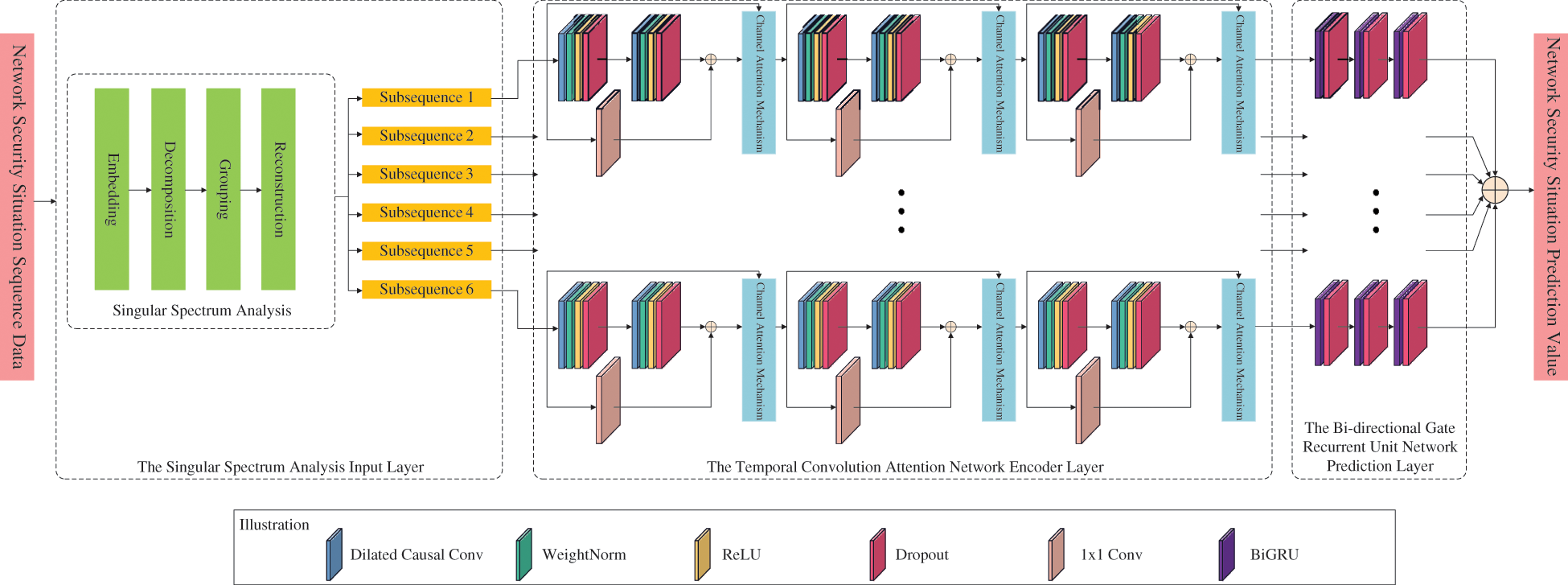
Figure 1: The model of NSSP based on TCAN-BiGRU optimized by SSA and IQPSO

2.1 The SSA Input Layer

In 1978 [16,17], Colebrook first proposed and used SSA in oceanographic research. It is mainly used to study non-linear time sequence data. It constructs the trajectory matrix from the time sequence obtained, which is decomposed and reconstructed to extract the long-term trend signal, periodic signal, noise signal, and other information. It mines the correlation between data and improves prediction accuracy to the maximum extent. The specific process of SSA includes four steps, embedding, decomposition, grouping, and reconstruction.

(1)   Embedding

The security data from the China National Computer Emergency Response Technology Coordination Center (CNCERT/CC) [18] were selected as experimental data comprising five security indicators. The situation value was obtained by weekly situation evaluation. Assuming the situation value of N-weeks is obtained, it was constructed into a time sequence S=SN=[s1,s2,…,sN]. The trajectory matrix was constructed according to Eq. (1).

S=[S1,S2,…,SK]=(si,j=1L,K)=[s1s2⋯sKs2s3⋯sK+1⋮⋮⋱⋮sLsL+1⋯sN](1)

where, K=N−L+1, si(1≤i≤N) is the situation value of N-weeks. Si=(si,…si+L−1)T (1≤i≤K) is the vector sequence with a length of L mapped from K-original time sequences. N is the length of the time sequence. L is the number of dimensions in the embedded space (or window length), generally L<N/2.

(2)   Decomposition

SSA adopts singular-value decomposition (SVD). In the defined matrix X=SST , ST  is the transposed matrix of S. λ1,…λL is set to the characteristic value of X. λ1≥⋯≥λL≥0 and U1,…,UL are the distinct vectors corresponding to λ1,…λL, respectively.

Let d=rank(S)=max{i,λi>0},Vi=ST Ui/λi(i=1,…,d), the trajectory matrix S can be expressed as:

S=S1+S2+⋯+Sd(2)

where, Si=λiUiViT . U and V are the left and right singular vectors of matrix S, respectively. {λi} is known as the singular spectrum of S.

(3)   Grouping

The subscript set {1,…,d} is divided into m disjoint subsets I1,I2,…,Im. Let I={i1,…,ip} the composite matrix corresponding to I is this SI=Si1+⋯+Sip. Therefore, the SVD of S of the trajectory matrix can be expressed as:

S=SI1+⋯+SIm(3)

(4)   Reconstruction

The reconstruction is mainly performed by the diagonal averaging method, which converts each matrix SIj in Eq. (3) into a decomposition sequence with a length of N.YL×K=(yij)(1≤i≤L,1≤j≤K),L∗=min(L,K),K∗=max(L,K). If L<K, yij∗=yijoryij∗=yji. The decomposition sequence (y1,y2,…,yN) is defined as:

yk={1k∑m=1kym,k−m+1∗,1≤k<L∗1L∗∑m=1L∗ym,k−m+1∗,L∗≤k≤K∗1N−k+1∑m=k−K∗+1N−K∗+1ym,k−m+1∗,K∗<k≤N(4)

The original sequence S can be decomposed into the sum of m time sequences with a length of N. The specific flow of data processed by SSA is shown in Fig. 2.

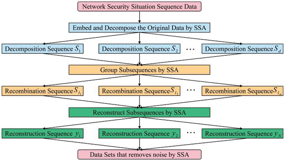
Figure 2: SSA flow chart

2.2 The TCAN Encoder Layer

The TCAN encoder layer is the superposition of the three-layer temporal convolution neural (TCN) network module and the channel attention module. Its structure is shown in Fig. 3. Each layer of dilated causal convolution has Fkconvolution kernels. The size of each convolution kernel is kd. The inflation factors of dilated causal convolution in three residual modules are d1, d2, and d3, respectively.

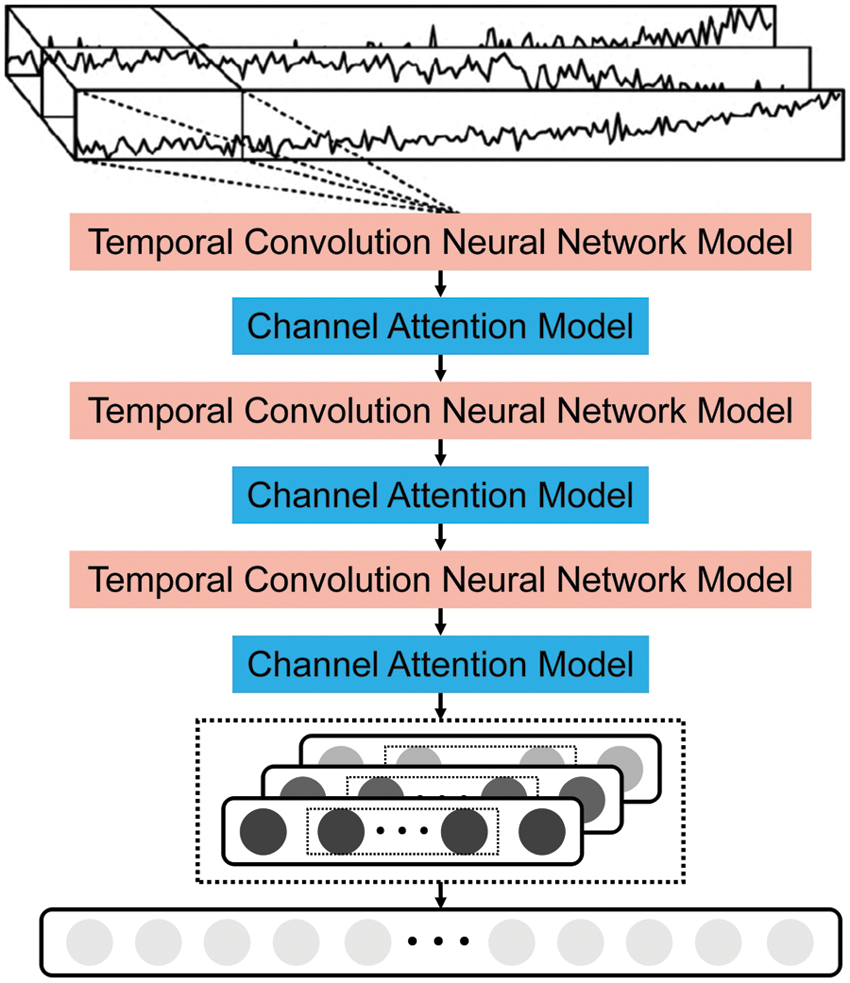
Figure 3: TCAN structure

Bai et al. [19] proposed TCN in 2018. It is mainly used for the processing of time sequence data. Compared with ordinary one-dimensional (1D) convolution, the TCN has two additional operations [20,21]: causal convolutions and dilated convolutions. Different network layers are connected with residuals to avoid gradient disappearance or explosion phenomena while extracting sequence features. The structure of its causal convolutions and dilated convolutions are shown in Fig. 4a. The residual module is shown in Fig. 4b.

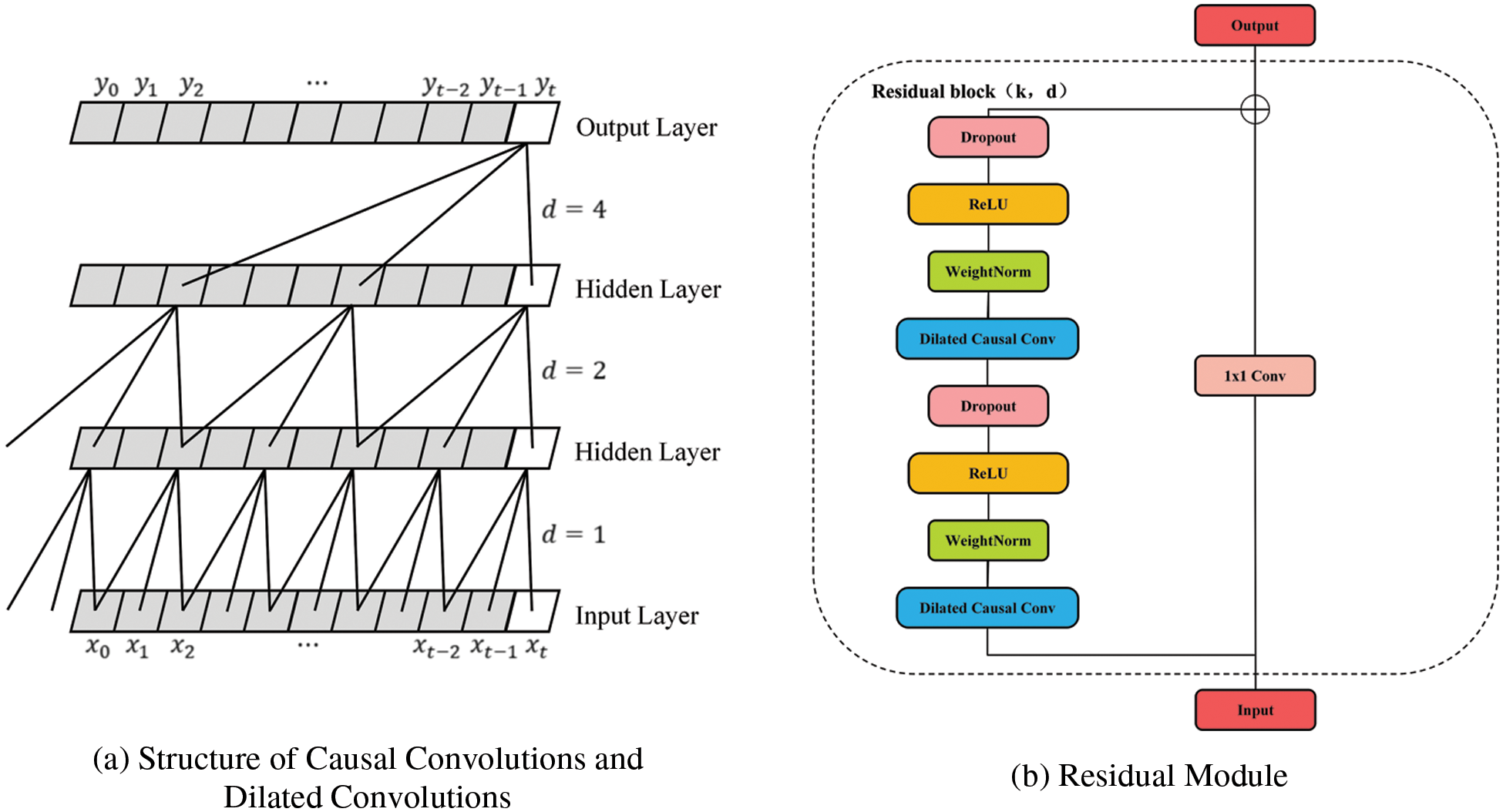
Figure 4: TCN model

This paper introduced TCN into NSSP. When its causal convolutions are used, it may successfully guarantee that information about the current situation is not “leaked” from the future to the past, maintaining the accuracy of the data. Using dilated convolutions can enable TCN to receive more comprehensive historical data with fewer layers and a more extensive receptive area. Network overfitting may be successfully stopped using the ReLU activation function, Dropout, and identity mapping network. Specifically, assuming that for a 1D sequence with an input of x∈Rn and a convolution kernel f:{0,…,k−1}→R, the dilated convolution operation F for the element s in the sequence is defined as:

F(s)=(x⋅df)(s)=∑i=0k−1f(i)⋅xs−d⋅i(5)

where, d is the inflation factor. k is the size of the convolution kernel. s−d⋅i denotes the direction of looking in the past. When dilated convolutions are used, d typically increases exponentially with the depth of the network layer i, i.e., d=O(2i) to ensure that the valid input of input time sequences is covered as the receptive field expands.

As the TCN’s receptive field depends on the network’s depth (n), the convolution kernel’s size (k), and the inflation factor (d), the addition of residual connections can keep the deep network stable. Its residual module is composed of network F and input x:

o=Activation(x+F(x))(6)

In reality, there is much redundant information in the time sequence information of network security situations. The performance of extracting model information will be disturbed if the redundant and essential information is equally treated. The attention mechanism has been one of the mainstream methods and research hotspots in current deep learning. It has been extensively used in various domains, including natural language processing, picture recognition, voice recognition, and other fields. The CAM is often used in computer vision to extract the mutual information between channels. The TCN herein is 1D convolution. As a result, the CAM should be improved. As shown in Fig. 5, in the CAM, the global information in different channels was first extracted by global max pooling (GMP) and global average pooling (GAP) to generate the corresponding output ml={ml1,ml2,…,mlk}andal={al1,al2,…,alk}.

mli=max(zl−1i)(7)

ali=1T∑j=1Tzl−1i,j(8)

where, zl−1i={zl−1i,1,zl−1i,2,…,zl−1i,T} denotes the output of the l−1th layer. l denotes the lth layer of the network. T is the time step, and i is the ith dimension channel of the output feature map.

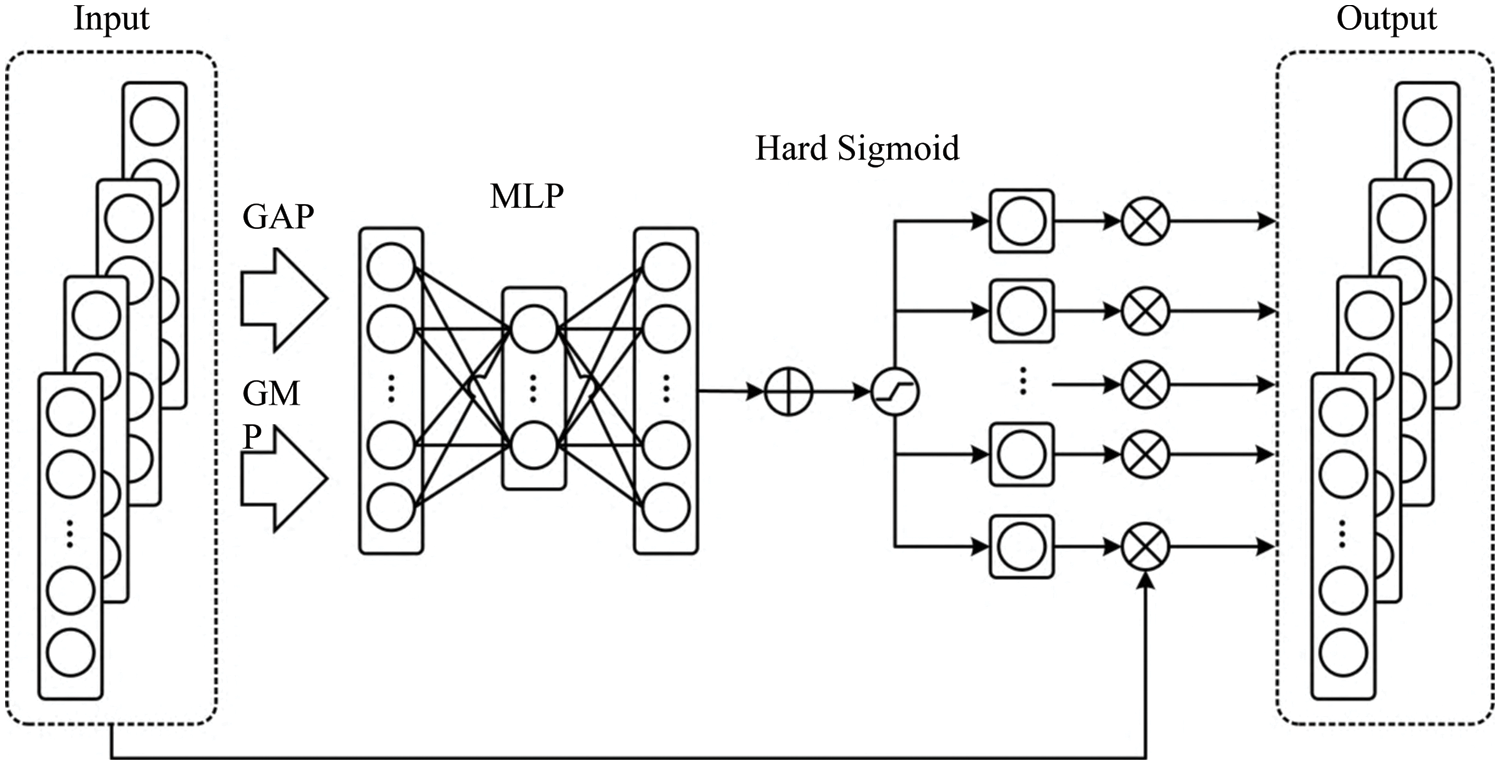
Figure 5: CAM module

The output features mi and ai were obtained by max pooling, and average pooling was placed in the multilayer perceptron (MLP) with a linear hidden layer. To reduce the parameter overhead in the network, the number of neurons in the hidden layer is k/r, where r is the decline rate, and k is the number of channels. The two groups of output features obtained via the MLP network were merged by element-wise summation. The hard sigmoid activation function normalized the merged output. The element-wise product was performed on the final output feature map and the original input to obtain the final output of the CAM module.

2.3 The BiGRU Network Prediction Layer

The BiGRU network prediction layer mentioned herein comprises three layers bi-directional gate recurrent unit (BiGRU) network. The number of neurons in the three layers is ln1, ln2, and ln3, respectively. All three layers BiGRU network are used to learn the before-and-after relationships of the network security situation. However, it is difficult to thoroughly learn the before-and-after relationships by relying only on a single-layer BiGRU network. Deepening the number of neural network layers can make the learning more adequate and improve the model prediction accuracy. Meanwhile. to avoid overfitting, a dropout layer was introduced after each layer BiGRU network to improve the neural network’s performance. Its structure is shown in Fig. 6.

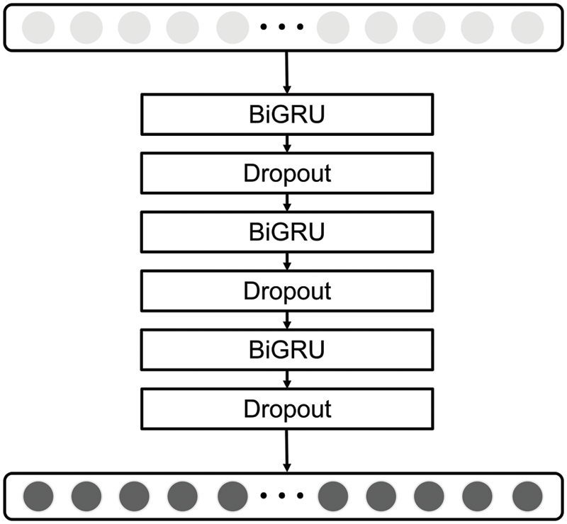
Figure 6: The structure of the BiGRU network prediction layer

The gate-recurrent unit (GRU) [22] is a common gate-recurrent neural network. GRU introduces the concepts of reset gate rt and update gate zt and modifies the calculation method of the hidden state h~t in the recurrent neural network [23]. Its internal structure is shown in Fig. 7.

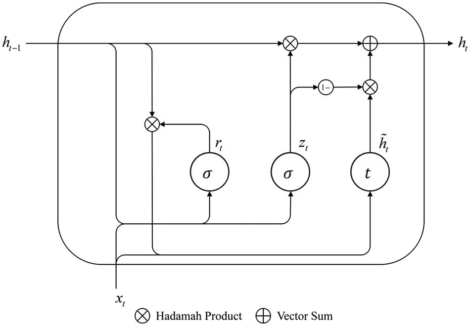
Figure 7: Basic structure of GRU

where, xt denotes the input information at the current moment. ht−1 and ht are the hidden statuses at the last and current moments, respectively. σ is the sigmoid activation function, and t is the tanh activation function.

The calculation equations for the GRU network are:

rt=σ(Wr⋅[ht−1,xt]+br)(9)

zt=σ(Wz⋅[ht−1,xt]+bz)(10)

h~t=tanh⁡(Wh~⋅[rt⋅ht−1,xt]+bh~)(11)

ht=(1−zt)⋅ht−1+zt⋅h~t(12)

yt=σ(Wo⋅ht+bo)(13)

where, W and b represent the weight matrix and bias term, respectively.

In NSSP, the network’s current state is related to the before and after state. The state information from after to before cannot be obtained if only TCAN is used. The BiGRU network was introduced herein to improve the prediction effect for NSSP.

BiGRU is formed by the forward and reversed superposition of GRUs. Its structure is shown in Fig. 8.

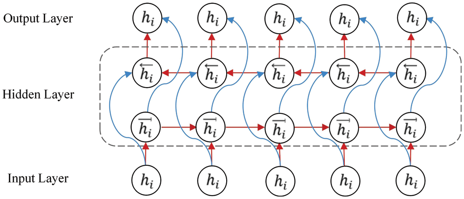
Figure 8: BiGRU network model

To determine the hidden layer status output H→={hL1,hL2,…,hLt}and H←={hRt,hRt−1,…,hR1}, the situation values of the forward and backward inputs were calculated using the forward and backward GRU networks, respectively. Afterward, the final output of the BiGRU network layer is obtained by splicing the forward and reverse hidden layer state output vectors:

H={H→,H←}(14)

2.4 Model Training Optimizer Algorithm

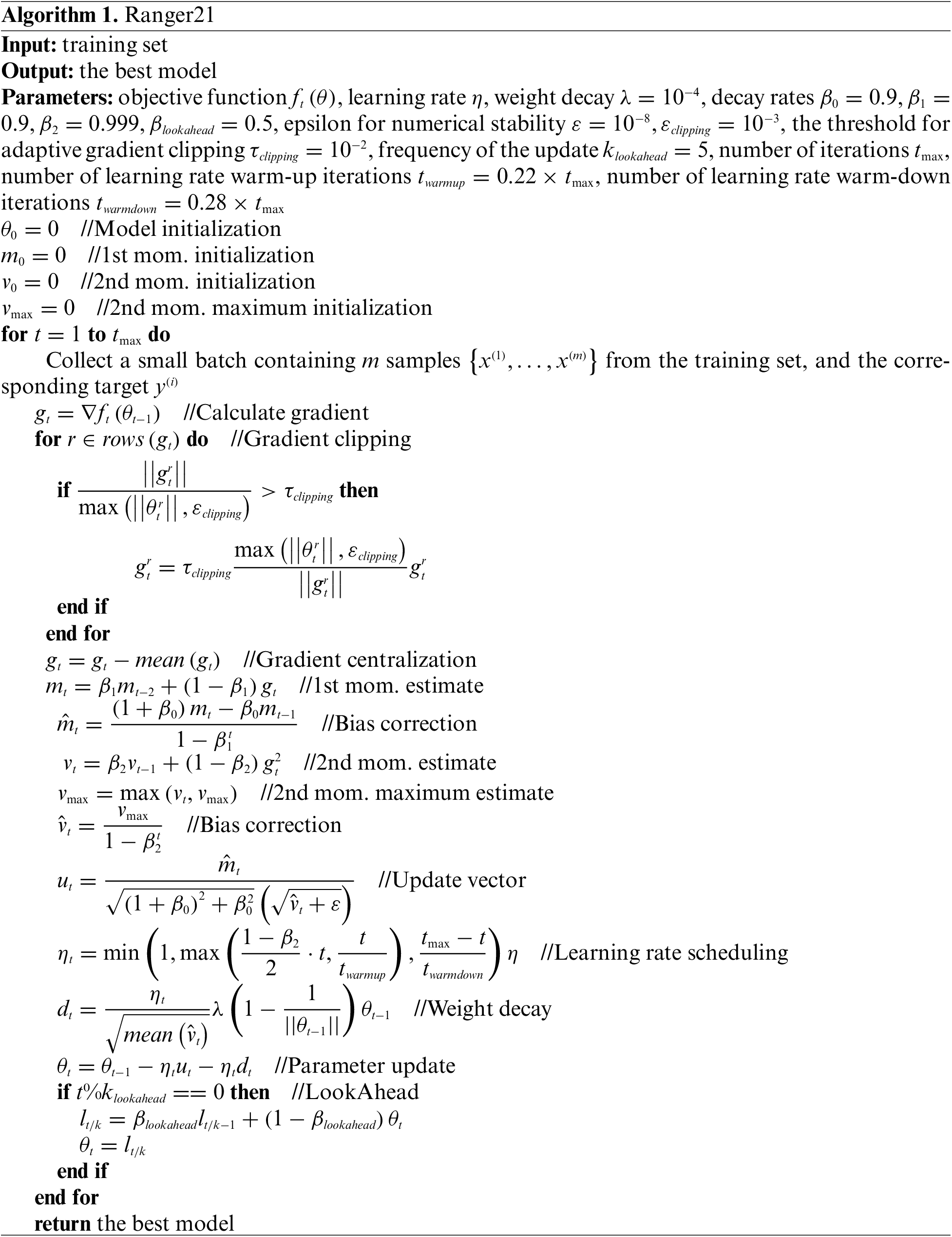
The TCAN-BiGRU model proposed herein adopts the Ranger21 optimizer algorithm [24,25] to solve the model parameters by solving the optimization problem of the cost function. Ranger21 combines AdamW [26], LookAhead [27], and eight other components. It integrates the advantages of AdamW for better generalization performance and the advantages of other components. See Algorithm 1 for the specific algorithm of Ranger21.

3  Improved Quantum Particle Swarm Optimization Algorithm

3.1 Particle Swarm Optimization

Particle swarm optimization (PSO) is a population-based optimization algorithm [28–31]. The term “population” describes several possible answers to an optimization issue. Every particle is a possible resolution. These particles move randomly through the problem space. Each particle will retain the fitness value associated with its prior best location (pbest). Also, each particle takes hold of the best location (gbest) discovered so far among all the particles in the population. Moreover, the final particle discovered in gbest is the best. Eqs. (15) and (16) in the PSO display particles’ speed vector and position vector adjustments of in D-dimensional space.

vij(t+1)=w⋅vij(t)+c1⋅r1(pij−xij)+c2⋅r2(pgj−pij)(15)

xij(t+1)=xij(t+1)+vij(t+1)(16)

where, w is the inertia factor. c1 and c2 are learning factors. r1 and r2 are two random numbers within the [0, 1] range. Xi=(xi1,xi2,…,xiD) means the position vector of the ith particle. Vi=(vi1,vi2,…,viD) represents the speed vector of the ith particle. Pi=(pi1,pi2,…,piD) means the previous best position of the ith particle, and the optimal fitness value in that position. Pg=(pg1,pg2,…,pgD) means the best position of all particles in the population. Each particle in the PSO converges to a focus point P=(p1,p2,…,pD) specified in Eq. (17) to guarantee the PSO’s convergence.

Pd=(c1⋅r1⋅pid+c2⋅r2⋅gd)/(r1+r2),d=1,2,…,D(17)

3.2 Quantum Particle Swarm Optimization

It is simple to slip into the local optimum trap because of classical PSO’s lack of randomization in particle location changes. In order to maximize the unpredictability of particle location by eliminating the traveling direction characteristic of particles, Sun Jun introduced quantum particle swarm optimization (QPSO) [32] in 2004.

The wave function Ψ(x⇀,t) of the QPSO represents the particle’s state. The likelihood that particles will arrive at the place x⇀ is represented by its squared value. Moreover, the Delta potential, with the point p⇀=(p1,p2,…,pD) at its core, constrains the quantum particles in the PSO, allowing them to converge to their local P-point without exploding. By resolving the Schrödinger equation, the probability density and distribution function are produced. The Monte Carlo approach may be used to determine the location of the ith particle. Equation provides its formulation (18).

xij=pj±Lij2 In(1/u)(18)

where, pj is the focal point to which particles converge. u is a random number within the [0, 1] range.

Lij(t+1)=2⋅β⋅|mbestj−x(t)ij|(19)

mbestj=1M∑i=1Mpij,j=1,2,…,D(20)

mbest=(mbest1,mbest2,…,mbestD)(21)

where, mbest denotes the mean best of all particles. β is the shrinkage and expansion coefficient. M is the population size. Therefore, Eq. (18) can be rewritten as:

xij(t+1)=pj±β⋅|mbestj−x(t)ij|⋅In(1/u)(22)

3.3 IQPSO

3.3.1 Chaotic Map

Initializing a population randomly in the typical quantum particle swarm optimization leads to a swift fall into the optimum local solution trap. It has a slow rate of convergence. With logistics mapping, the population is started in a chaotic order. In order to increase the efficiency and convergence rate of this method, the optimized variables are handled with the ergodicity of chaotic motion for optimum solution search.

The Logistics mapping is as follows:

Unγ+1=aUnγ(1−Unγ)(23)

where, n denotes the serial number of the chaotic variable. γ denotes the serial number of the population to be optimized. Unγ denotes the chaotic variable. a denotes the chaotic attractor, here a = 4.

3.3.2 Crossover Operator

The genetic algorithm is the source of the crossover operator. In the genetic algorithm, the crossover operation is used to exchange information between the chromosomes’ genes to keep good genes and allow them to develop into better genes. To broaden the population and enhance the algorithm’s ability to leap out of the local optimum, the longitudinal crossover operator was added to the QPSO in this study.

An arithmetic crossing between two distinct dimensions of a particle in a population is known as a “vertical crossover.” The problem that elements of different dimensions have different value ranges is solved by normalization. Meanwhile, each operation only generates one progeny particle, and only one dimension is updated.

Assuming that X(i) the d1th and d2th dimensions are involved in vertical crossover, the mean solution MSvc(i,d1) is generated according to Eq. (24).

MSvc(i,d1)=r⋅X(i,d1)+(1−r)⋅X(i,d2)(24)

where, i∈N(1,M), d1,d2∈N(1,D), r∈[0,1], MSvc(i,d1) is the d1th dimension offspring of the d1th and the d2th dimension of the individual particle X(i) generated by vertical crossover.

The conventional crossover operator chooses the crossover probability pcand executes crossover and mutation with a certain probability. One of the key elements that influence an algorithm’s capacity for optimization is the crossover probability. The production of new individuals slows down during iteration if pc is too tiny, which causes the calculation to end early. If pc is too big, the population will produce too many new individuals, harming any outstanding individuals who have already been produced. Therefore, seeking an adaptive crossover and mutation probability is vital for optimizing the algorithm. The adaptive crossover probability of a genetic algorithm improved the following formula:

pc={(pc1−pc2)(fmax−f′)fmax−favg,f′≥favgpc1,f′<favg(25)

where, pc1 and pc2 are constants. f’ represents the fitness value of a relatively excellent individual between the two individuals in which the crossover operation occurs. f represents the fitness function value of the particle on which the mutation operation occurs. favg means the current mean of the fitness function of the whole population.

3.3.3 Flow of IQPSO

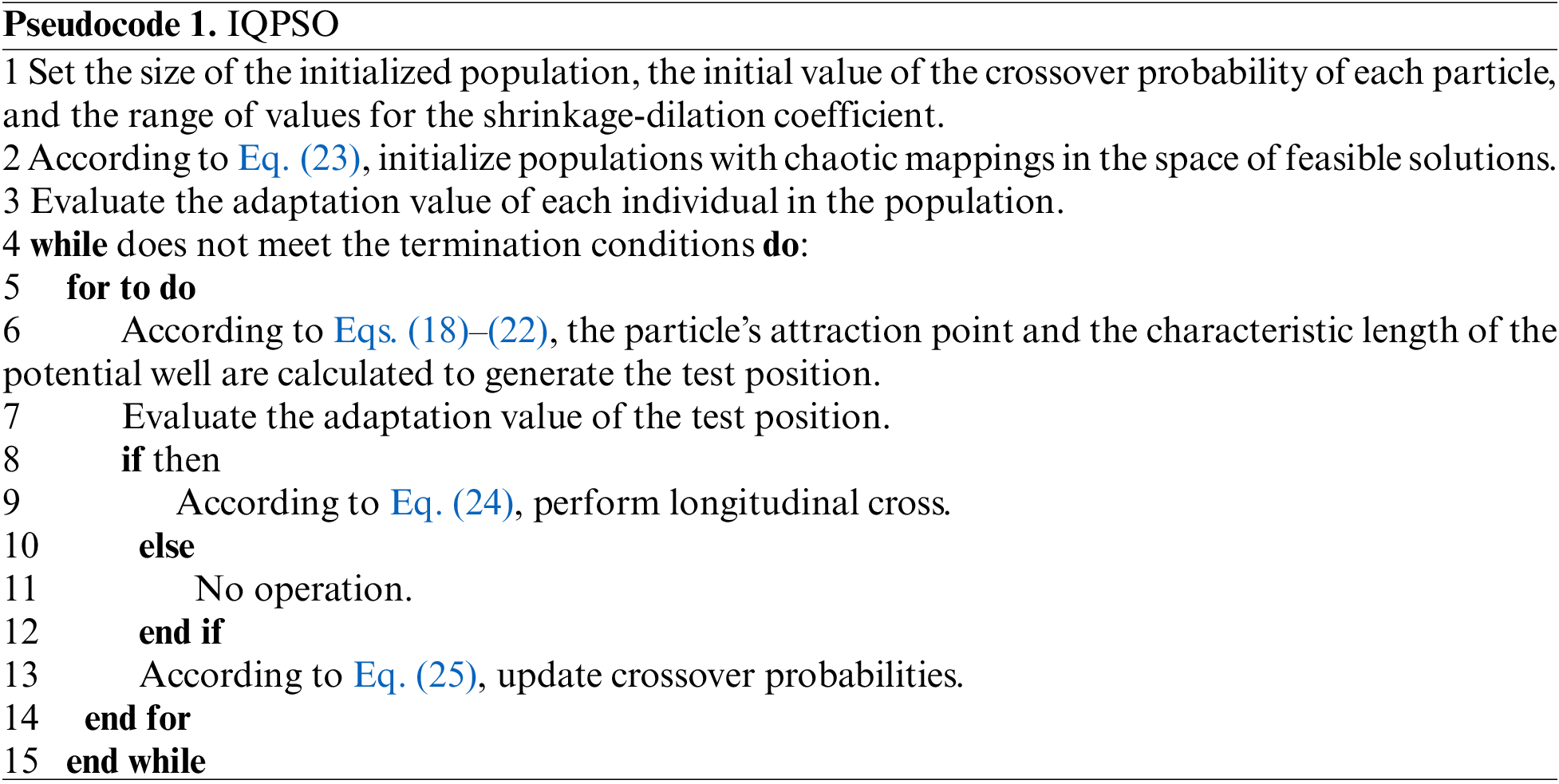
The IQPSO is shown in Fig. 9. See Pseudocode 1 for the specific algorithm of IQPSO.

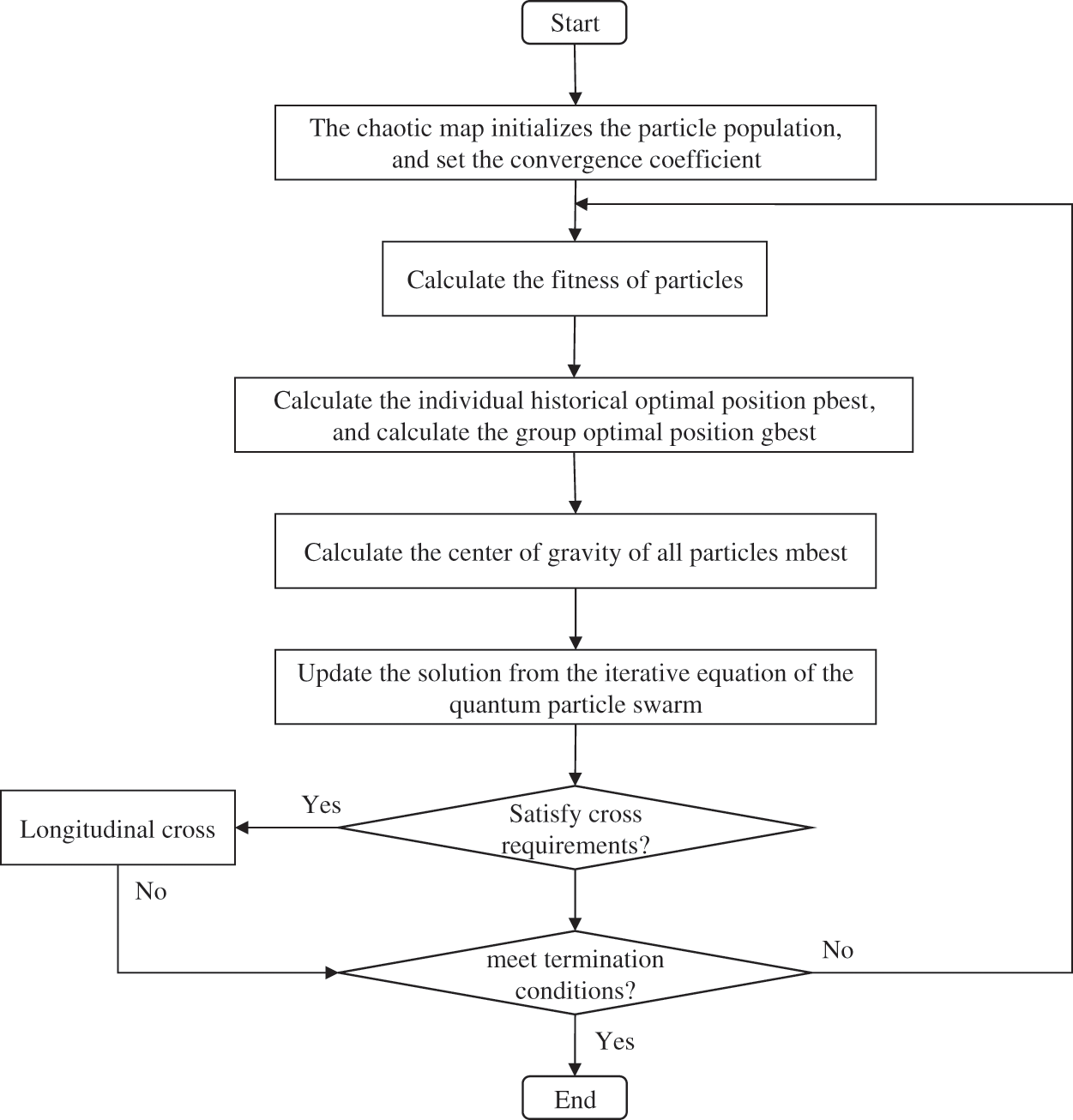
Figure 9: Flow chart of IQPSO

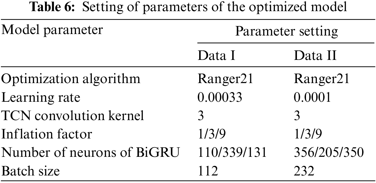
3.3.4 Hyperparameter of Optimization Model of IQPSO

In practical applications, different selections of hyperparameters will affect the training results of the model. The five hyperparameters in the model (number of neurons of the three-layer BiGRU, batch size, and optimizer’s learning rate) were optimized by the IQPSO in this paper to find the optimal solution to the model parameters. The algorithm flow is as follows:

Step 1: Data on the state of network security is read, cleaned, normalized, and processed with sliding windows before the training set and test set are split.

Step 2: Determine the topology of the model.

Step 3: The population is initialized by the chaotic map. In the population, each particle represents weight and offset. The fitness function is the mean absolute error of the training samples, and chaotic variables are added to the starting population.

Step 4: Establish the input model for the training set and evaluate the fitness of each particle according to the predicted value obtained.

Step 5: Compute the fitness value of particles, the population’s optimal location, the best historical position for each individual, and the center of gravity for every particle.

Step 6: Update the solution according to Eq. (22).

Step 7: Perform genetic coding on samples and carry out the longitudinal crossover operation on Eq. (24) according to the adaptive crossover probability of Eq. (25).

Step 8: Update the new generation of particle swarm.

Step 9: Calculate the fitness value of the new generation of particles.

Step 10: Achieve the desired number of repetitions or confirm that the termination requirements have been satisfied. If so, the iteration should end or go to Step 5.

Step 11: Use the particle with the final optimal fitness value as the hyperparameter of the model.

Step 12: Apply to optimal the hyper-parameter obtained to the model for prediction to get results.

4  Experimental Results and Analysis

4.1 Performance Evaluation of IQPSO

4.1.1 Benchmark Functions

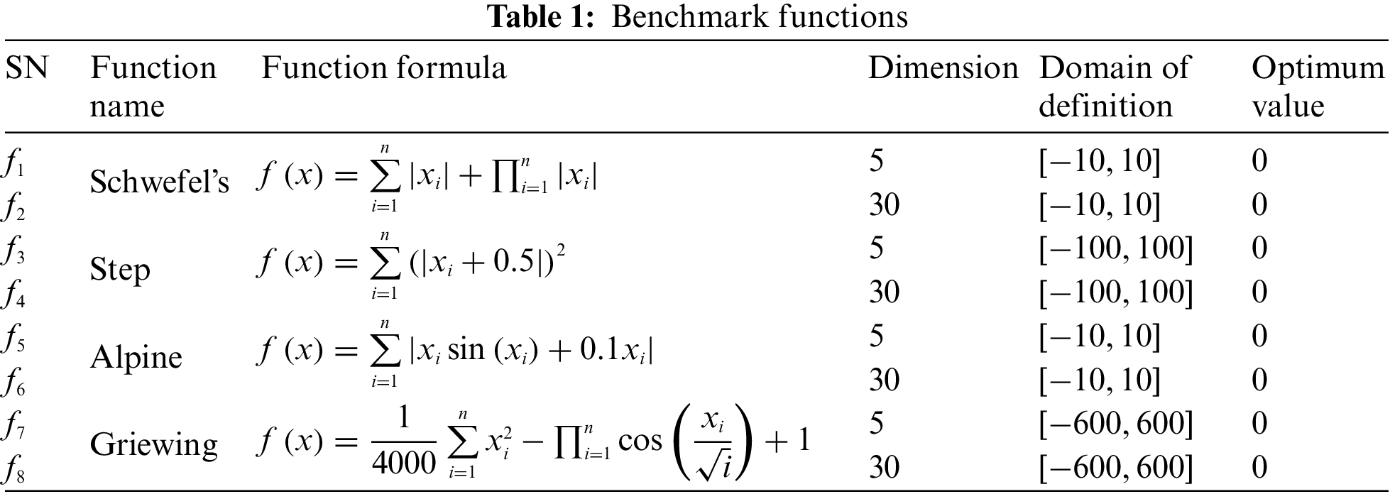
To verify the optimization ability and feasibility of the algorithm improved herein, this paper selected four test functions comparing this algorithm with the genetic algorithm (GA), traditional particle swarm optimization (PSO), traditional quantum particle swarm optimization (QPSO), crossover particle swarm optimization (CPSO) and crossover quantum particle swarm optimization (CQPSO) in different dimensions. The specific test functions are listed in Table 1. Where, f1 and f3 are low-dimensional unimodal functions. f2 and f4 are high-dimensional unimodal functions. f5 and f7 are low-dimensional multimodal functions. f6 and f8 are high-dimensional multimodal functions. Unimodal functions only have one optimum global point and no local extreme point, primarily for the test function convergence rate. The performance of functions that jump out of the local extreme point in many dimensions is observed using multimodal functions with numerous local extreme points.

4.1.2 Analysis of Simulation Results

The parameters in algorithms and functions in the test were set as follows: The population size was 30. The maximum number of iterations was 200. The shrinkage and expansion coefficient was 0.6. The maximum crossover probability was 0.8. Each benchmark function was selected to run independently 50 times to avoid excessive accidental errors. The optimum values, means, and standard deviations were taken as evaluation indexes. The optimum value is the highest or most favorable value of a particular variable or set of variables. A mean is an average of a set of numerical values or quantities. Standard deviation (SD) measures how spread out numbers are in a data set. The experimental results are shown in Table 2.

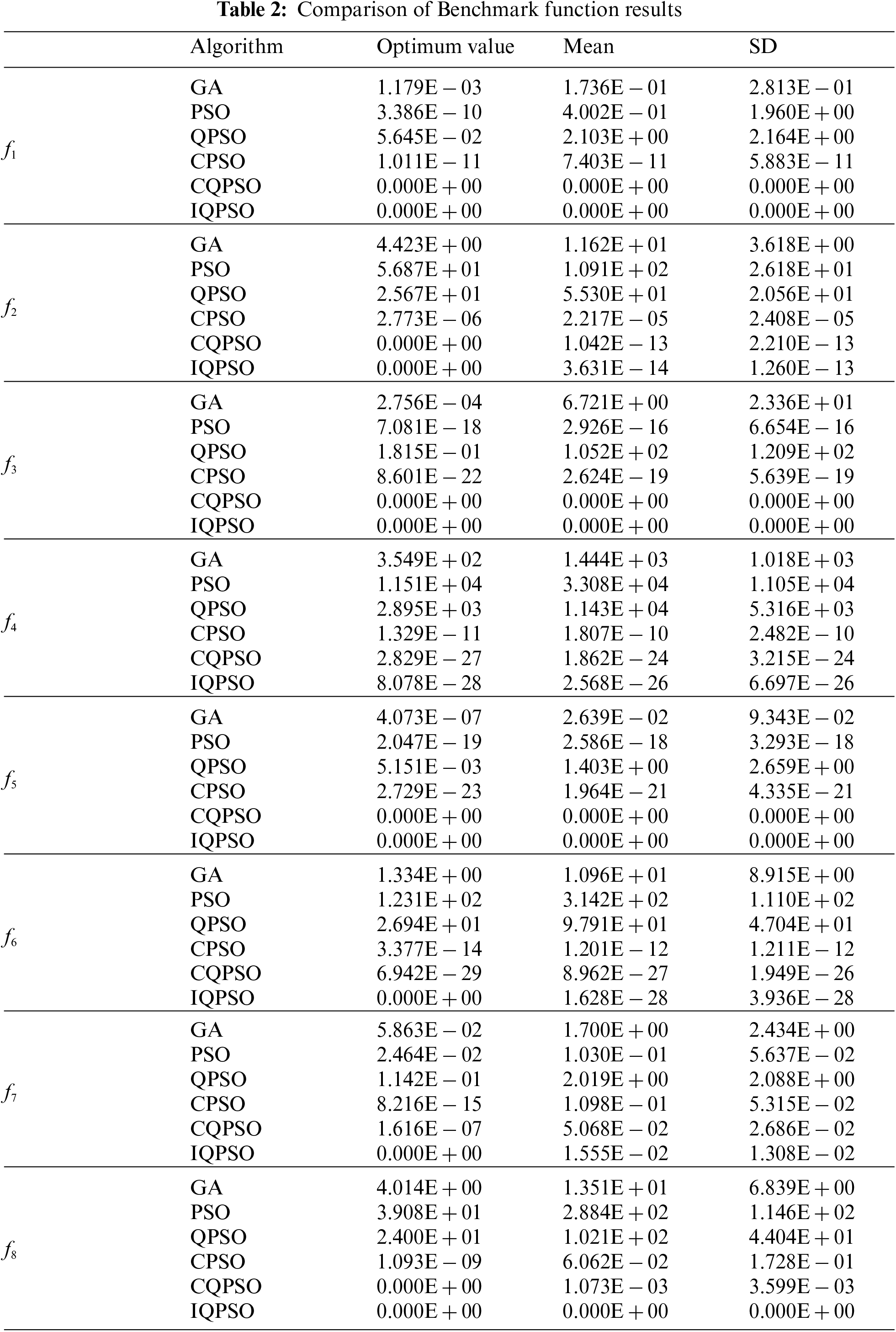
In the two low-dimensional unimodal functions, CQPSO and IQPSO found the theoretical optimum value of 0 when solving f1 and f3 functions. Meanwhile, the SD was also 0, showing the algorithm’s advantages. In the two high-dimensional unimodal functions, CQPSO and IQPSO found the theoretical optimum value of 0 when solving the f2 function, but the mean and SD of IQPSO were smaller than CQPSO’s. When the f4 function was solved, the optimum value, mean, and SD obtained by IQPSO were improved by at least one order of magnitude compared with those obtained by the other five algorithms. The stability was higher than that of other algorithms. In the two low-dimensional multimodal functions, the advantages of CQPSO and IQPSO were higher and more stable for the f5 function solution than the other four algorithms. Only IQPSO could reach the theoretical optimum value for the f7 function solution, but its ability was equivalent to that of the other five algorithms. In the two high-dimensional multimodal functions, IQPSO could find the theoretical optimum value when solving the f6 function, but its stability needed improvement. When solving the f8 function, IQPSO could reach the theoretical optimum value, and the SD was 0. Besides, only CQPSO could find the theoretical optimum value, but its stability must be revised.

According to the research, unimodal functions had greater solution accuracy than multimodal functions for each method. In comparison to high-dimensional functions, low-dimensional functions have greater solution accuracy. IQPSO demonstrated superior optimization accuracy and stability than the other five methods, independent of unimodal or multimodal and high-dimensional or low-dimensional functions.

4.1.3 Analysis of Convergence Curves

Experiments were carried out on eight functions with six algorithms to compare the convergence rate of six algorithms intuitively. The eight average convergence curves in Fig. 10 were obtained.

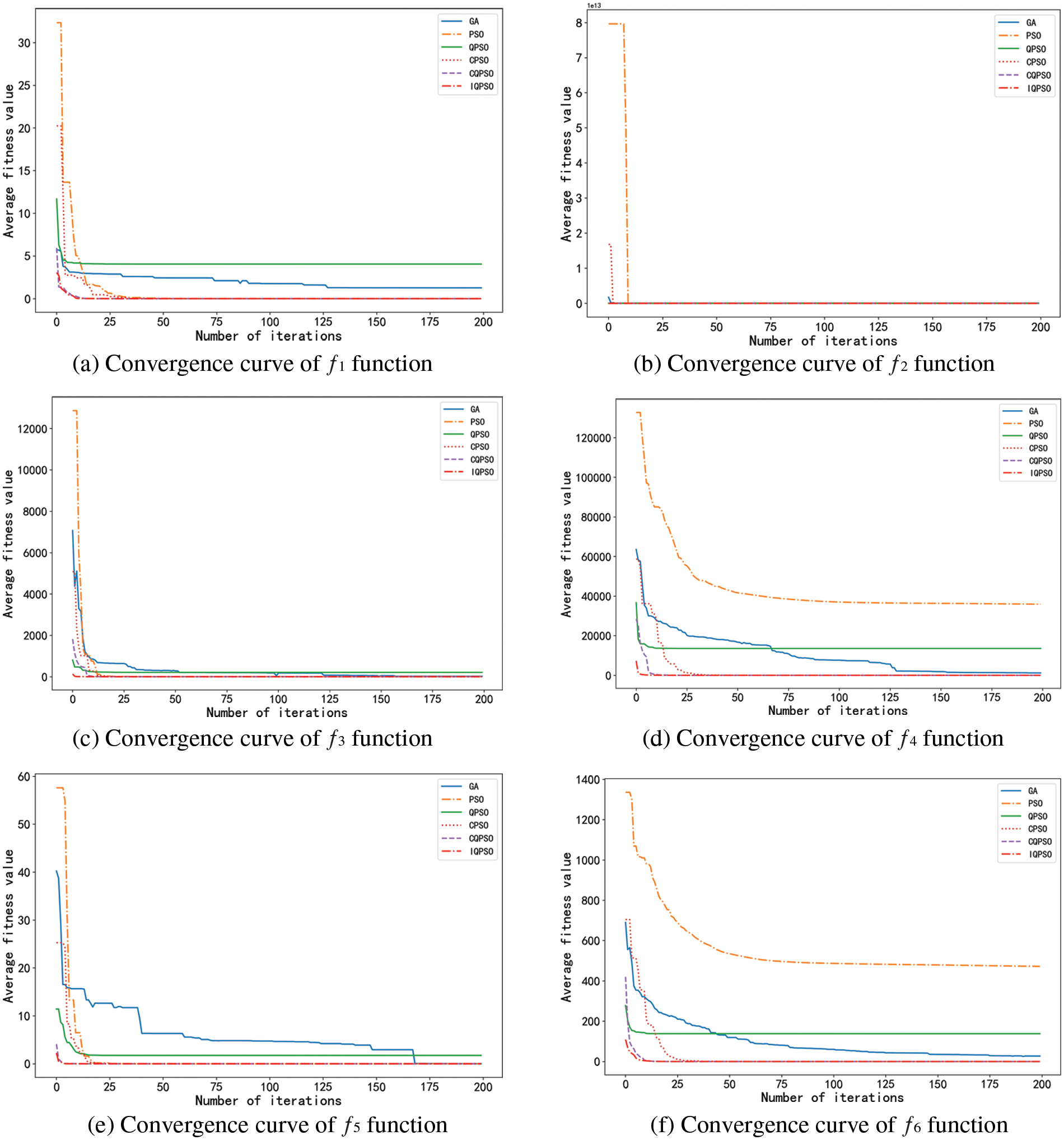
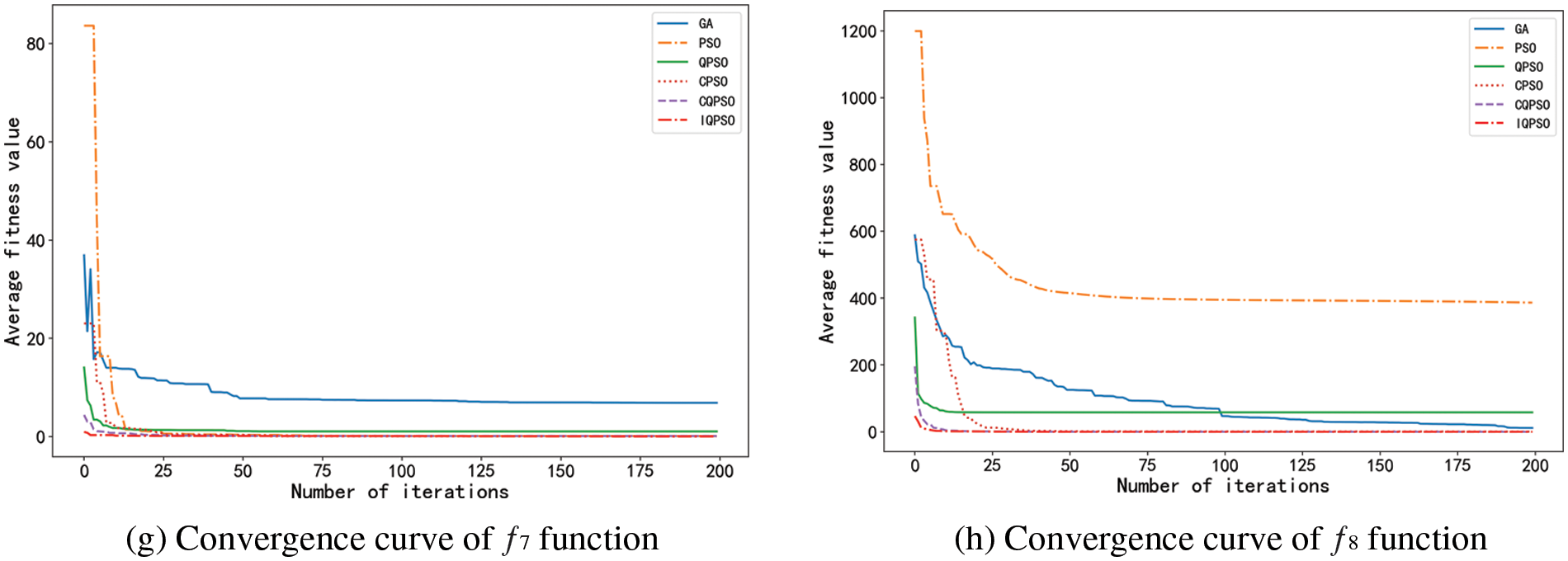
Figure 10: Mean convergence curves of Benchmark functions

The eight graphs above clearly show each algorithm’s fitness value changes in the optimization process. In these graphs, the convergence rate of IQPSO is relatively higher, and its convergence accuracy is much higher than that of other algorithms, showing the advantages of algorithm improvement.

4.1.4 Wilcoxon Rank Sum Test Analysis

A statistical test should be carried out for the performance evaluation of enhanced algorithms, according to Ref. [33]. In other words, it is not sufficient to compare the benefits and drawbacks of algorithms based just on the mean and SD. The suggested enhanced algorithms must pass the statistical test to demonstrate that they are significantly better than other algorithms already in use. Independently compare the results of each test to reflect the stability and fairness of algorithms. The Wilcoxon rank sum test, with a significance threshold of 5%, was employed in this study to determine if the findings of IQPSO were statistically different from the best results of the other five algorithms. The hypothesis should be rejected when the p-value is less than 5% since it shows that the comparison algorithms differ significantly from one another. If not, the hypothesis should be accepted, proving that the comparison algorithms’ capacity to optimize is equivalent. Table 3 lists the rank sum test p-value of IQPSO and the other five algorithms under eight functions. The NAN in the table denotes “not applicable” since no comparison is available when the two comparison algorithms arrive at the optimal value. That is, it is impossible to assess the relevance. R is the outcome of a decision of significance. “+”, “–” and “=” signify that IQPSO’s performance when compared to other algorithms is better, worse, or equal.

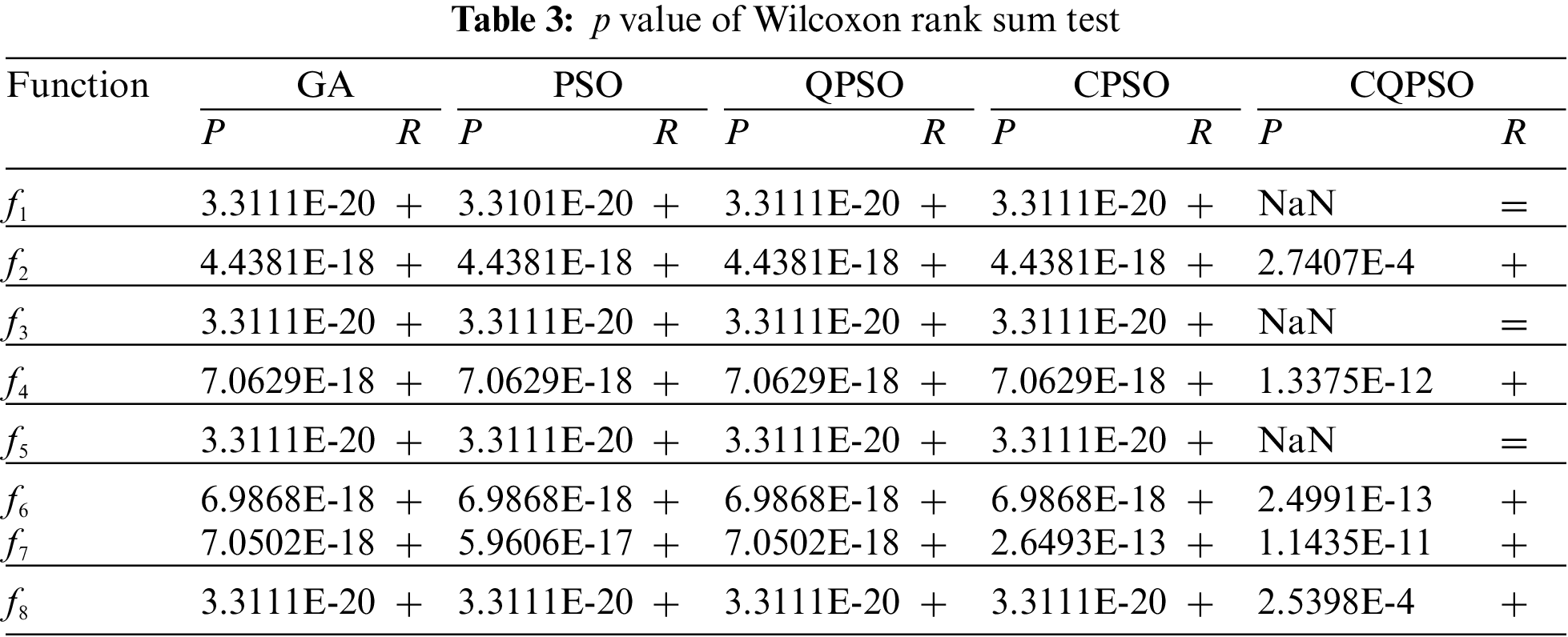
It can be seen from Table 3 that most p-value is much less than 5%, which shows that IQPSO has significant advantages over the other five algorithms. In comparing IQPSO and CQPSO, the R-value in f1, f3, and f5 functions is “=.” This is because CQPSO has good optimization performance. IQPSO and CQPSO can find the optimum value.

4.2 NSSP Analysis

4.2.1 Selection of Network Security Situation Data and Environment Configuration

Two data sets were selected for experiments to verify the situation prediction algorithms proposed in this paper. The two sets of data are specified as follows:

Data I: The experimental data obtained from the network environment built in Ref. [34] was adopted to obtain exact and practical network security situation value in this study: the number, type, and severity of attacks on the host were comprehensively evaluated through the network security evaluation system every 30 min to calculate the network security situation value of the current period. Finally, 150 situation values were selected for normalization. The resultant sample data of this experiment are shown in Fig. 11a.

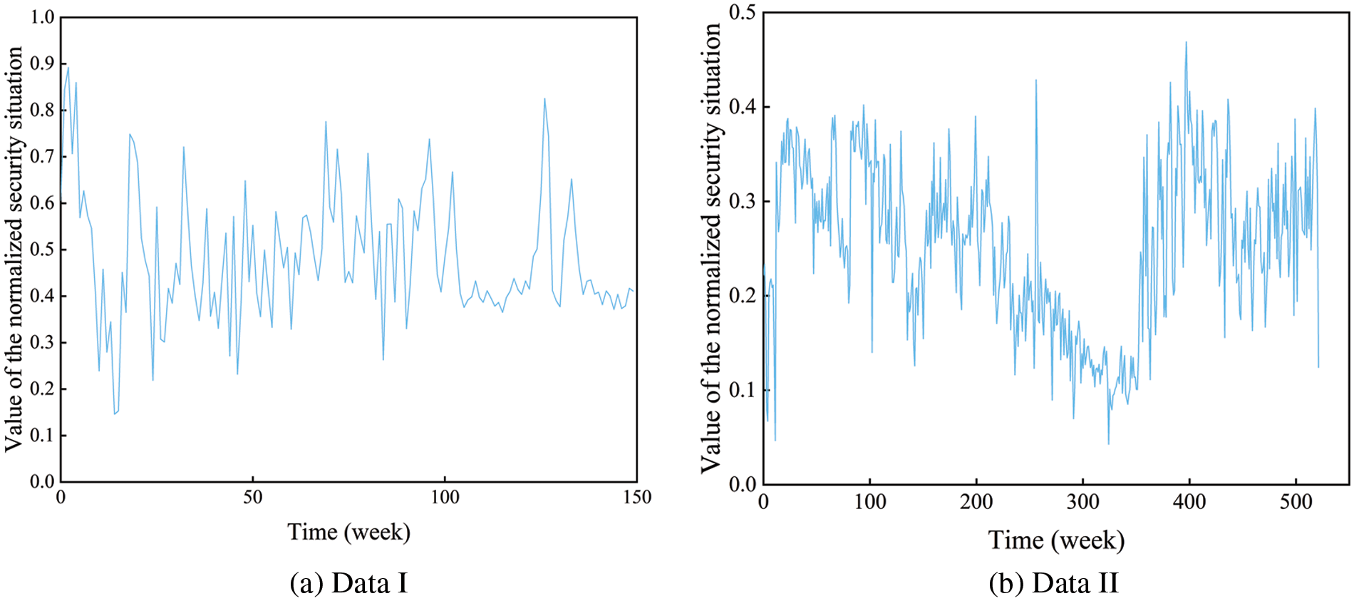
Figure 11: Network security situation value

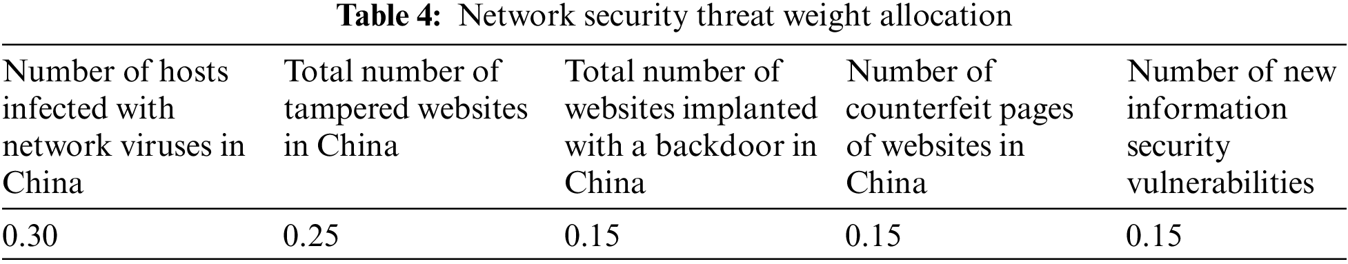
Data II: The experimental premise was the weekly security situation data that the CNCERT/CC publishes. From the website’s 30th issue in 2012 to its 29th issue in 2022, 522 issues of weekly situation data were chosen as the foundation for experimental verification. The data were mainly evaluated from five perspectives. The scenario evaluation approach from Ref. [35] was used in this article for quantization in order to accurately portray the network security state. As illustrated in Table 4, different weights were allocated based on the severity of network security risks. The weekly circumstance value was then determined using Eq. (26).

SA=∑i=15NTiNTimax⋅ωi(26)

where, NTi represents the number of a particular network security threat in a specific week (i represents the type of security threat). NTimax represents the maximum number of this security threat in the 522 issues of data selected. ωi is the corresponding weight.

Data normalization can reduce the variance of features to a specific range, reduce the influence of outliers, and improve the convergence rate of the model. This paper normalized the characteristic data to the interval [−1, 1] by the min-max normalization method. The calculation formula is as follows.

x′=x−min(x)max(x)−min(x)(27)

where, x’ is the data of x mapped to the [−1, 1] range. min(x)andmax(x) are the minimum and the maximum of the data set. The calculated network security situation value is shown in Fig. 11b.

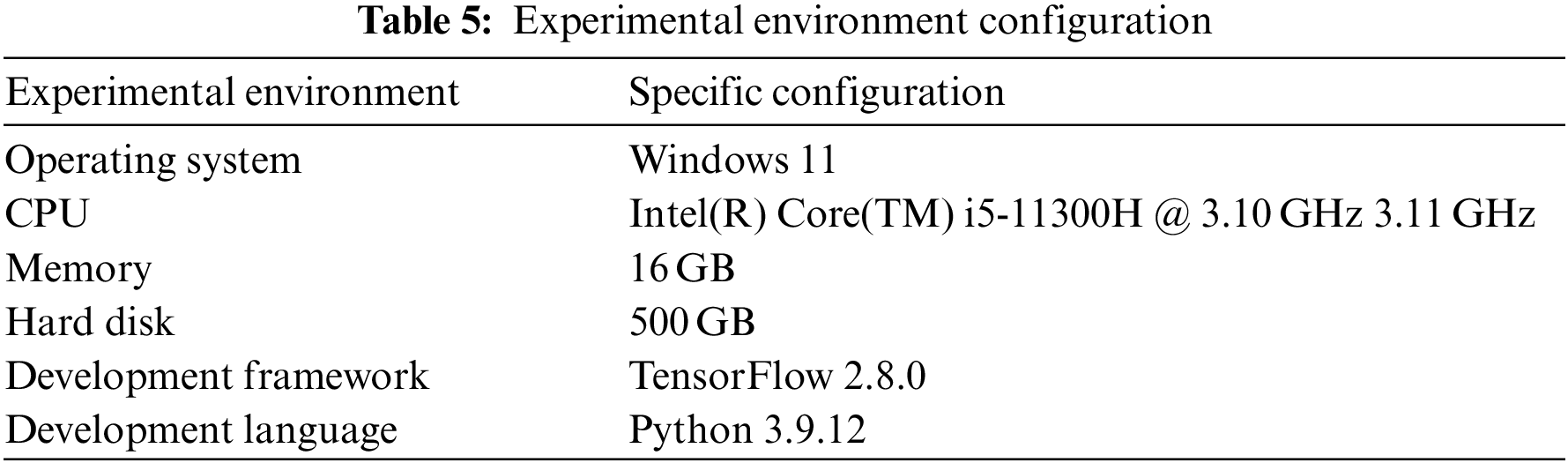
The TCAN-BiGRU model and all the experiments were carried out under the TensorFlow deep learning framework. The specific experimental environment [36] is shown in Table 5.

4.2.2 Experimental Evaluation Criteria

To evaluate the effect of the prediction models proposed herein, three parameters, the mean absolute error (MAE), the mean square error (MSE), and the coefficient of determination (R2) were selected as evaluation indexes [37]. The calculation formula for these indexes is as follows:

MAE=1N∑i=1N|yi−y^i|(28)

MSE=1N∑i=1N(yi−y^i)2(29)

R2=[∑i=1N(yi−y¯)(y^i−y^¯i)]2[∑i=1N(yi−y¯)2][∑i=1N(y^i−y^¯i)2](30)

In the above three equations, yi is the true value of a sample. y^i is the predicted value of a sample. N is the number of samples. y¯i is the mean of true values. y^¯i is the mean of predicted values.

4.2.3 Selection of Different Optimizer Algorithms

To verify the effectiveness of the Ranger21 algorithm selected in this paper, it was compared with Adam [38], SGD [39], and Adagrad [40] optimizer algorithms by experiments. The comparison of predictions on different data sets by different optimizer algorithms is shown in Fig. 12.

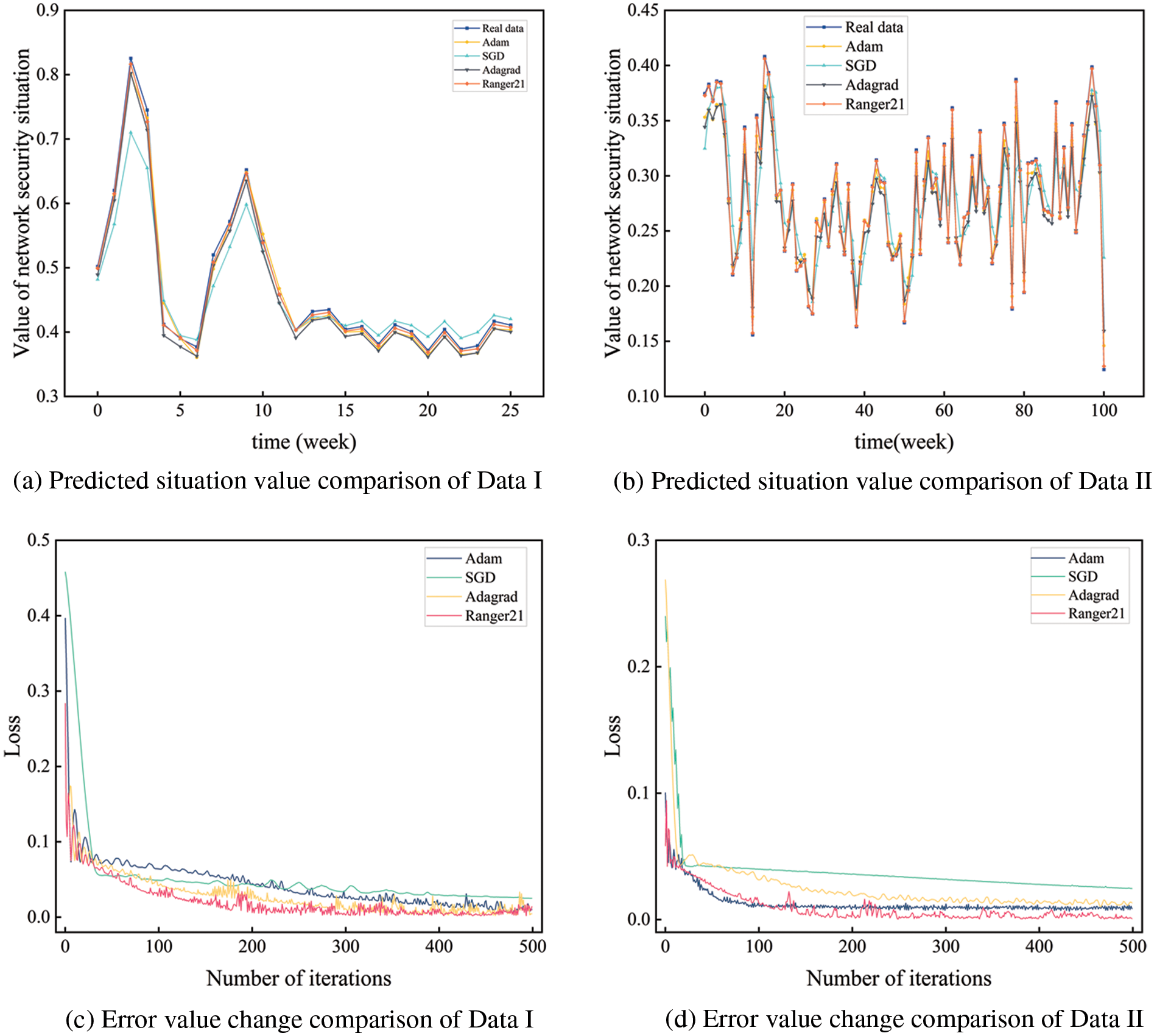
Figure 12: Comparison of predictions by different optimizer algorithms

It can be seen from the figure that compared with the Adam algorithm, SGD algorithm, and Adagrad algorithm, the Ranger21 algorithm has a higher convergence rate for network training. Moreover, its prediction fitting degree is higher than that of the other three optimization algorithms. Experimental results showed that the Ranger21 algorithm could promote the optimization of network training.

4.2.4 Selection of Optimal Model Parameters

To better realize the prediction effect, the IQPSO was adopted in this paper to optimize these hyper-parameters to find the optimal solutions to model parameters. The IQPSO-associated parameters were set as follows: The population size was 5; the number of iterations was 30; the shrinkage and expansion coefficient was 0.6; and the maximum crossover probability was 0.8.

To increase the convergence rate and prevent the aimless search of particles in the search space, the bounds of optimization parameters are now set as follows: The number of BiGRU neurons is taken in the [10, 500] range. The batch size is taken in the [100, 1000] range. The optimizer’s learning rate is taken in the [0.0001, 0.005] range.

The training results of the TCAN-BiGRU model optimized by IQPSO are shown in Fig. 13. The training error converges and becomes stable with the updating of the algorithm, verifying the effectiveness of IQPSO.

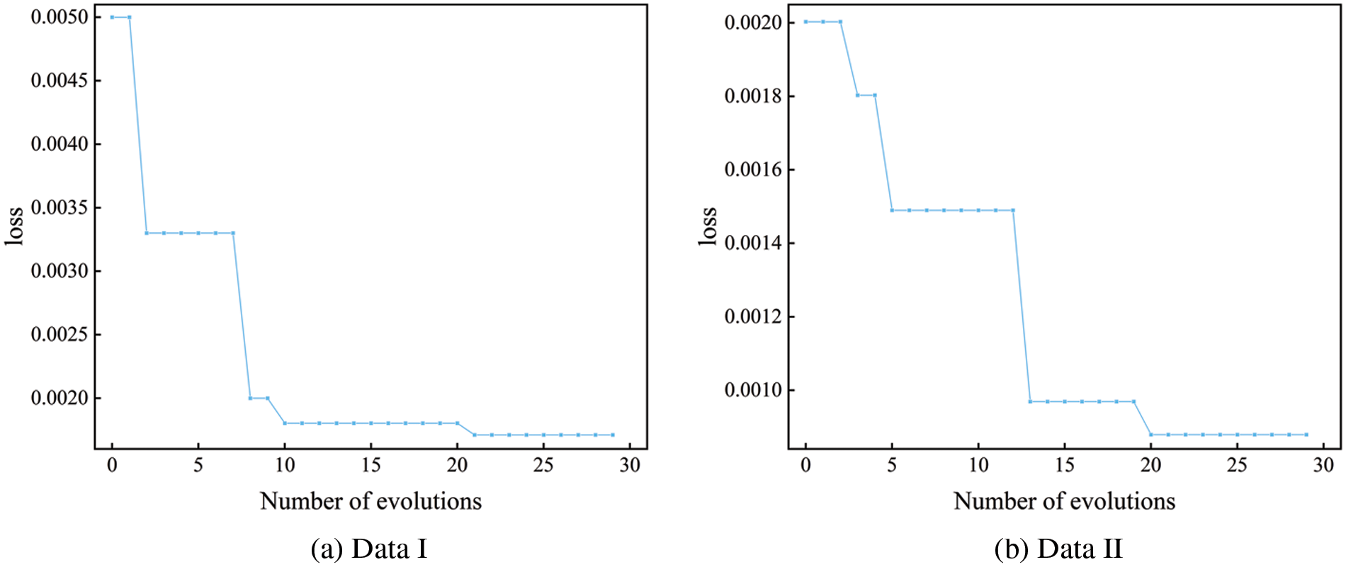
Figure 13: Changes in hyper-parameters of the TCAN-BiGRU model optimized by IQPSO

The parameters of the network model optimized by the IQPSO are shown in Table 6.

4.2.5 Analysis of Experimental Prediction Results

The model provided here was tested against both conventional machine learning techniques and deep learning techniques, such as the BP, LSTM, GRU, TCN, BiGRU, and IQPSO-TCAN-BiGRU models, to see how well it performed in the NSSP.

SSA of Experimental Data

After the SSA of the network security situation value, it was embedded, decomposed, grouped, and reconstructed into six subsequences. The results are shown in Fig. 14.

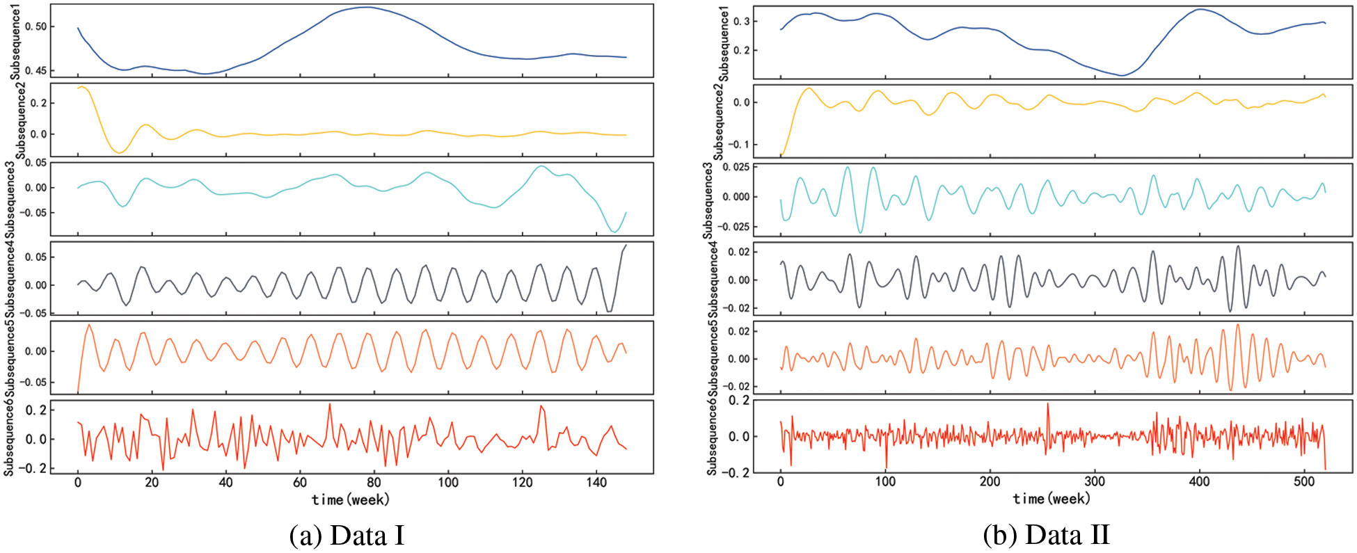
Figure 14: Results after SSA

It is commonly accepted that the high-frequency component, such as subsequence 4, subsequence 5, and subsequence 6, shows the random effect of the network security situation based on the subsequence characteristics of the decomposed network security scenario data sequence. Several low-frequency elements, including subsequences 1, 2, and 3, can be seen as periodic elements of the network security status data sequence since they exhibit strong sinusoidal fluctuation characteristics. The network security situation’s low-frequency portion is a trend indicator that may be used to identify the long-term trend in network security.

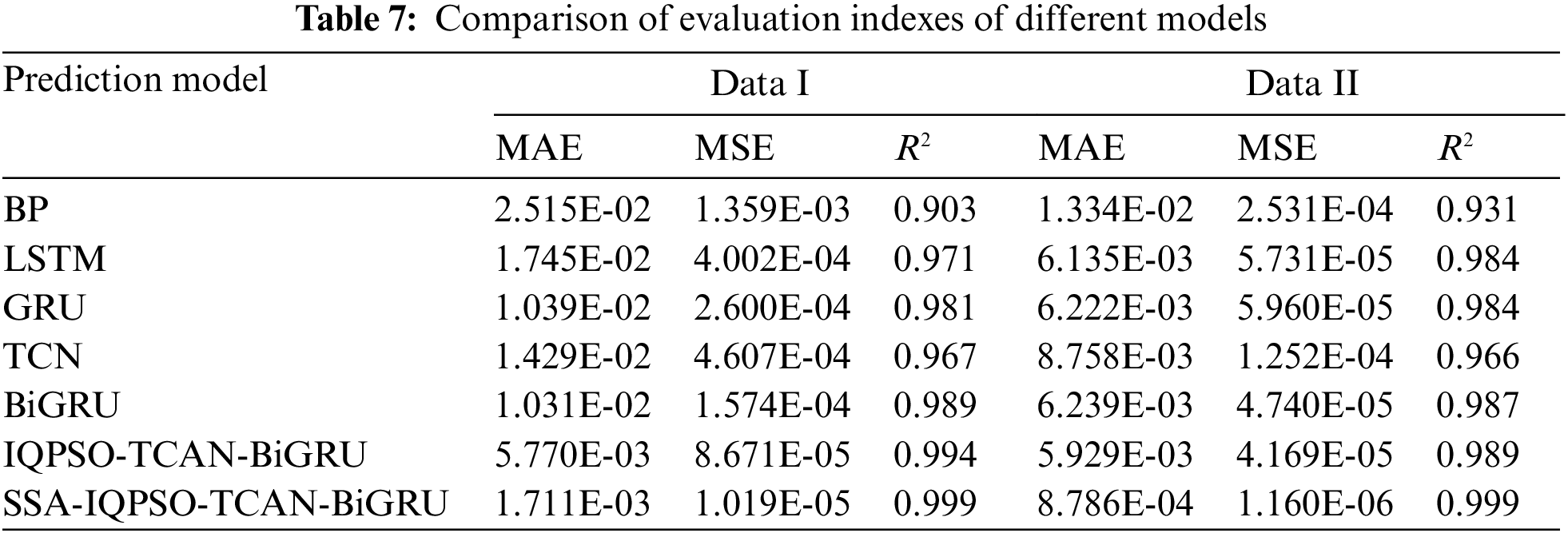
Comparison of Prediction Accuracy

To evaluate the predictive ability of models as a whole, the MAE, MSE, and R2 of different models were calculated. The results are listed in Table 6. To make the comparison fairer, multiple experiments were conducted on all prediction models to take the mean. According to Table 7, the error of the SSA-IQPSO-TCAN-BiGRU model is over one order of magnitude lower than other models than the IQPSO-TCAN-BiGRU model. In terms of error, it has significant advantages over the IQPSO-TCAN-BiGRU model. The degree of fitting of the SSA-IQPSO-TCAN-BiGRU model is more than 0.5% higher than that of other models. Overall, it is shown that the SSA-IQPSO-TCAN-BiGRU model is effective in predicting network security situation data.

The predicted and true values of the SSA-IQPSO-TCAN-BiGRU model and BP, LSTM, GRU, TCN, BiGRU, and IQPSO-TCAN-BiGRU prediction models are compared in Fig. 15. The closer the predicted value curve of each model is to the actual value, the better the model effect is proved. Intuitively, all prediction models have certain predictive abilities. The predicted and true values of the SSA-IQPSO-TCAN-BiGRU model have the highest degree of the fitting. Its predicted values almost coincide with true values at each prediction point.

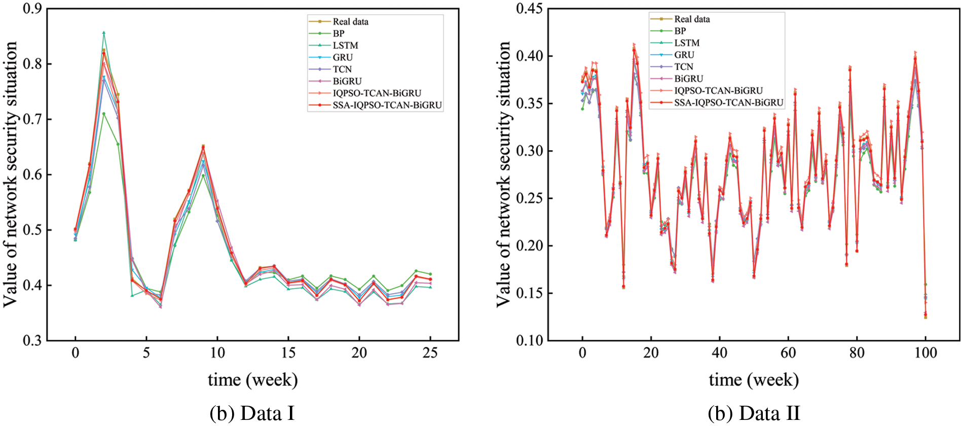
Figure 15: Comparison of situation value prediction by different models

Convergence Analysis

Fig. 16 displays the curves of model training error with the number of iterations. Every curve can reach convergence and stability. This chart shows that the prediction model presented here is more accurate and has a higher convergence rate than previous models, demonstrating that it can completely understand the characteristics of temporal data and produce valuable results.

Figure 16: Curves of model training error with the number of iterations

Runtime Analysis

The models make predictions while taking into account both the accuracy of the forecast and the amount of time needed to run the model, i.e., the time for model training and the time for the prediction. The complexity of the model, the number of iterations, and the batch size all affect how long it takes to run. Table 8 displays the execution timings of several prediction models discovered through experimentation.

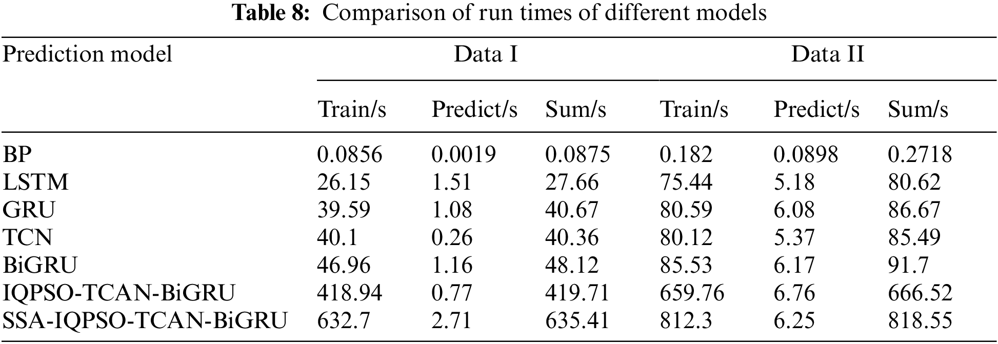
As can be seen from Table 7, the BP model takes less time. However, it is easier to process the data and obtain lower prediction accuracy of the results, and we need help to predict the posture values accurately. The IQPSO-TCAN-BiGRU model and the model proposed in this paper are optimized by IQPSO and take longer training time, but the prediction time remains relatively stable. The model proposed in this paper improves the prediction accuracy while the prediction time spent is the same.

5  Conclusions

Multi-attribute security indicators were fused based on network security situation data. In this paper, SSA was introduced into network security prediction. A series of subsequences were obtained by embedding, decomposing, grouping, and reconstructing the network security situation values obtained weekly. Afterward, the prediction model of the TCAN-BiGRU network was established for each subsequence. Finally, the prediction results of subsequences were superposed to obtain the final NSSP value. Meanwhile, the QPSO was improved. The chaotic map and crossover operator were introduced to ensure population diversity. Besides, adaptive crossover probability was adopted to improve the algorithms’ convergence accuracy and rate. In this paper, it was proved with different data and by multiple experiments that the model has strong feature extraction ability, high prediction accuracy, and prediction efficiency when network security situation data are processed, whose coefficient of determination is up to 0.999 on both sets, indicating that the model proposed herein is effective and practical. In subsequent studies, the cutting-edge deep learning model and swarm intelligence optimization algorithm will be focused on further improving the effectiveness of this model in actual applications.

Funding Statement: This work is supported by the National Science Foundation of China (61806219, 61703426, and 61876189), by National Science Foundation of Shaanxi Provence (2021JM-226) by the Young Talent fund of the University, and the Association for Science and Technology in Shaanxi, China (20190108, 20220106), and by and the Innovation Capability Support Plan of Shaanxi, China (2020KJXX-065).

Conflicts of Interest: The authors declare that they have no conflicts of interest to report regarding the present study.

References

1. V. O. Nyangaresi, A. J. Rodrigues and S. O. Abeka, “ANN-FL secure handover protocol for 5G and beyond networks,” in AFRICOMM 2020: Towards New E-Infrastructure and E-Services for Developing Countries: 12th EAI Int. Conf., Ebène City, Mauritius, vol. 361, Springer, pp. 99–118, 2021. [Google Scholar]

2. J. B. Lai, H. Q. Wang and L. Zhu, “Study of network security situation awareness model based on simple additive weight and grey theory,” in 2006 Int. Conf. on Computational Intelligence and Security, vol. 2, Guangzhou, China, IEEE, pp. 1545–1548, 2006. [Google Scholar]

3. D. H. Kim, T. Lee, S. O. D. Jung, H. P. Ln and H. J. Lee, “Cyber threat trend analysis model using HMM,” in Third Int. Symp. on Information Assurance and Security, Manchester, UK, IEEE, pp. 177–182, 2007. [Google Scholar]

4. P. Baruah and R. B. Chinnam, “HMMs for diagnostics and prognostics in machining processes,” International Journal of Production Research, vol. 43, no. 6, pp. 1275–1293, 2005. [Google Scholar]

5. Q. Q. Luo, Research of Network Security Situation Awareness Based on D-S Evidence Theory. Nanjing: Nanjing University of Posts and Telecommunications, pp. 38–53, 2021. [Google Scholar]

6. Q. M. Wei, Y. B. Li and Y. L. Ying, “Network security situation prediction based on dempster-shafer evidence theory and recurrent neural network,” Journal of University of Jinan(Science and Technology), vol. 34, no. 3, pp. 238–246, 2020. [Google Scholar]

7. Z. C. Li, Z. G. Chen and J. Tang, “Prediction of network security situation on the basis of time series analysis,” Journal of South China University of Technology(Natural Science Edition), vol. 44, no. 5, pp. 137–143, 2016. [Google Scholar]

8. P. Yang, Z. C. Ma, D. Jin, B. Y. Meng and W. F. Jiang, “Evaluation model of network situation and its awareness prediction oriented to intelligent power grid,” Journal of Lanzhou University of Technology, vol. 41, no. 4, pp. 105–109, 2015. [Google Scholar]

9. Y. J. Deng, Z. C. Wen and X. W. Jiang, “Prediction method of network security situation based on grey theory,” Journal of Hunan University of Technology, vol. 29, no. 2, pp. 69–73, 2015. [Google Scholar]

10. J. Yu, Z. X. Lin and B. Xie, “Network security situation awareness prediction method based on grey correlation model,” Research and Exploration in Laboratory, vol. 38, no. 2, pp. 31–35, 2019. [Google Scholar]

11. D. Preethi and N. Khare, “Sparse auto encoder driven support vector regression based deep learning model for predicting network intrusions,” Peer-to-Peer Networking and Applications, vol. 14, no. 4, pp. 2419–2429, 2021. [Google Scholar]

12. R. Zhang, M. Liu, Y. Y. Yin, Q. K. Zhang and Z. Y. Cai, “Prediction algorithm for network security situation based on BP neural network optimized by SA-SOA,” International Journal of Performability Engineering, vol. 16, no. 8, pp. 1171–1182, 2020. [Google Scholar]

13. J. Zhu and T. T. Wang, “Network security situation prediction based on improved WGAN,” in Simulation Tools and Techniques: 11th Int. Conf., Chengdu, China, pp. 654–664, 2019. [Google Scholar]

14. W. Ni and N. Guo, “Network security situation prediction with temporal deep learning,” in 2020 Int. Conf. on Image, Video Processing and Artificial Intelligence, Shanghai, China, SPIE, vol. 11584, pp. 475–480, 2020. [Google Scholar]

15. B. Xi, G. Zhao, M. Chao and J. Wang, “A prediction model of cloud security situation based on evolutionary functional network,” Peer-to-Peer Networking and Applications, vol. 13, no. 5, pp. 1312–1326, 2020. [Google Scholar]

16. K. Afshar and N. Bigdeli, “Data analysis and short term load forecasting in Iran electricity market using singular spectral analysis (SSA),” Energy, vol. 36, no. 5, pp. 2620–2627, 2011. [Google Scholar]

17. C. L. Wu and K. W. Chau, “Rainfall-runoff modeling using artificial neural network coupled with singular spectrum analysis,” Journal of Hydrology (Amsterdam), vol. 399, no. 3–4, pp. 394–409, 2011. [Google Scholar]

18. CNCERT/CC, Weekly Report on Network Security Information from 2012 to 2022, Beijing, China: CNCERT/CC, 2022. [Online]. Available: https://www.cert.org.cn/publish/main/index.html [Google Scholar]

19. S. Bai, J. Z. Kolter and V. Koltun, “An empirical evaluation of generic convolutional and recurrent networks for sequence modeling,” ArXiv Preprint, arXiv: 1803.01271, 2018. [Google Scholar]

20. P. Hewage, A. Behera, M. Trovati, E. Pereira, M. Ghahremani et al., “Temporal convolutional neural (TCN) network for an effective weather forecasting using time-series data from the local weather station,” Soft Computing, vol. 24, no. 21, pp. 16453–16482, 2020. [Google Scholar]

21. R. J. Zhang, F. Sun, Z. W. Song, X. L. Wang, Y. C. Du et al., “Short-term traffic flow forecasting model based on GA-TCN,” Journal of Advanced Transportation, vol. 2021, pp. 1–13, Article ID 1338607, 2021. [Online]. Available: https://doi.org/10.1155/2021/1338607 [Google Scholar] [CrossRef]

22. R. Zhao, D. Z. Wang, R. Q. Yan, K. Z. Mao, F. Shen et al., “Machine health monitoring using local feature-based gated recurrent unit networks,” IEEE Trans. on Industrial Electronics, vol. 65, no. 2, pp. 1539–1548, 2017. [Google Scholar]

23. Z. Z. Han, M. Y. Shang, Z. B. Liu, C. M. Vong, Y. S. Liu et al., “SeqViews 2 SeqLabels: Learning 3D global features via aggregating sequential views by RNN with attention,” IEEE Trans. on Image Processing, vol. 28, no. 2, pp. 658–672, 2018. [Google Scholar]

24. L. Wright and N. Demeure, “Ranger21: A synergistic deep learning optimizer,” ArXiv Preprint, arXiv: 2106.13731, 2021. [Google Scholar]

25. L. Y. Liu, H. M. Jiang, P. C. He, W. Z. Chen, X. D. Liu et al., “On the variance of the adaptive learning rate and beyond,” ArXiv Preprint, arXiv: 1908.03265, 2019. [Google Scholar]

26. I. Loshchilov and F. Hutter, “Fixing weight decay regularization in Adam,” in Int. Conf. on Learning Representations (ICLR 2018), Vancouver, BC, Canada: Vancouver Convention Center, 2018. [Google Scholar]

27. M. R. Zhang, J. Lucas, J. Ba and G. E. Hinton, “Lookahead optimizer: K steps forward, 1 step back,” in Advances in Neural Information Processing Systems (NeurIPS 2019), Vancouver, BC, Canada: Vancouver Convention Center, 2019. [Google Scholar]

28. A. Carlisle and G. Dozier, “An off-the-shelf PSO,” in Proc. of the Workshop on Particle Swarm Optimization, Indianapolis, Purdue School of Engineering and Technology, 2001. [Google Scholar]

29. S. Zhou, W. Pan, B. Luo, W. L. Zhang and Y. Ding, “A novel quantum genetic algorithm based on particle swarm optimization method and its application,” Acta Electronica Sinica, vol. 34, no. 5, pp. 897–901, 2006. [Google Scholar]

30. J. M. T. Wu, G. Srivastava, A. Jolfaei, M. Pirouz and J. C. W. Lin, “Security and privacy in shared HitLCPS using a GA-based multiple-threshold sanitization model,” IEEE Trans. on Emerging Topics in Computational Intelligence, vol. 6, no. 1, pp. 16–25, 2021. [Google Scholar]

31. P. Cheng, J. F. Roddick, S. C. Chu and C. W. Lin, “Privacy preservation through a greedy, distortion-based rule-hiding method,” Applied Intelligence, vol. 44, pp. 295–306, 2016. [Google Scholar]

32. J. Sun, B. Feng and W. B. Xu, “Particle swarm optimization with particles having quantum behavior,” in Proc. of the 2004 Congress on Evolutionary Computation (IEEE Cat. No. 04TH8753), Portland, OR, USA, IEEE, vol. 1, pp. 325–331, 2004. [Google Scholar]

33. J. Derrac, S. García, D. Molina and F. Herrera, “A practical tutorial on the use of nonparametric statistical tests as a methodology for comparing evolutionary and swarm intelligence algorithms,” Swarm & Evolutionary Computation, vol. 1, no. 1, pp. 3–18, 2011. [Google Scholar]

34. Y. Jiang, C. H. Li, X. H. We and Z. P. Li, “Research on improving PSO optimized RBF for network security posture prediction,” Measurement and Control Technology, vol. 37, no. 5, pp. 56–60, 2018. [Google Scholar]

35. W. F. Jiang, Research on Network Security Posture Prediction Based on Multi-Model Weight Extraction and Fusion, Lanzhou: Lanzhou University of Technology, 2016. [Google Scholar]

36. J. F. Sun, C. H. Li and Y. F. Song, “Network security situation prediction based on CCQPSO-BiLSTM,” in 2022 Int. Conf. on Image Processing, Computer Vision and Machine Learning (ICICML), Xi’an, China, IEEE, pp. 445–451, 2022. [Google Scholar]

37. G. Wang, “Comparative study on different neural networks for network security situation prediction,” Security and Privacy, vol. 4, no. 1, pp. e138, 2021. [Google Scholar]

38. I. K. M. Jais, A. R. Ismail and S. Q. Nisa, “Adam optimization algorithm for wide and deep neural network,” Knowledge Engineering and Data Science, vol. 2, no. 1, pp. 41–46, 2019. [Google Scholar]

39. Y. J. Wang, P. Y. Zhou and W. Y. Zhong, “An optimization strategy based on hybrid algorithm of Adam and SGD,” in MATEC Web of Conf., Shanghai, China, EDP Sciences, vol. 232, pp. 03007, 2018. [Google Scholar]

40. A. Lydia and S. Francis, “Adagrad—An optimizer for stochastic gradient descent,” Int. J. Inf. Comput. Sci, vol. 6, no. 5, pp. 566–568, 2019. [Google Scholar]