Cloud Resource Integrated Prediction Model Based on Variational Modal Decomposition-Permutation Entropy and LSTM

1  Introduction

The purpose of cloud computing to provide various resource services is to timely and accurately meet the resource needs of multiple users. However, the resource requirements of users are constantly changing, and sometimes the fluctuations are very violent, and we may not implement the provision of resources in time. Therefore, we need to quickly and accurately predict the cloud resource demand to respond in advance and help service providers choose appropriate physical servers, improving resource utilization and ensuring service quality. We can accurately predict future resource demand while ensuring a good user experience. Therefore, it is necessary to use accurate prediction algorithms to predict application resource requirements. This way, resource changes can be predicted in advance to quickly and accurately respond to resource supply.

By analyzing many historical resource conditions, cloud resource forecasting can predict future resource requirements. Moreover, container cloud workloads have been proven to be significantly correlated with working hours so that we can transform cloud resource forecasting problems into the cloud resource time series data analysis problem-sequence data analysis problems. Linear prediction methods for cloud resource time series, such as the differential regression model [1], and exponential smoothing model [2–5], are very effective in predicting linear stationary time series data. Moreover, with the increase in the complexity and scale of cloud resource clusters, the randomness and volatility of historical data are apparent, so the linear methods with poor performance are far from being able to solve the prediction problems of high complexity and volatility. For solving the complexity of non-stationary data prediction, genetic algorithms and various neural network algorithms [6–11] have been proven to solve the problems of time series data volatility effectively, prediction accuracy, and data complexity.

Since the container cloud historical data is non-stationary by some factors, to reduce the influence of non-stationarity on the prediction accuracy. We can use signal decomposition technology to decompose the original data into residual components and a plurality of relatively stable intrinsic mode functions and then reconstruct and predict the sub-modes, which can improve the prediction accuracy effectively. Reference [12] based on wavelet supported and Savitzky–Golay filtering random configuration network integration to predict future workloads and decomposed into multiple components for prediction. References [13–15] all use the foundation and improved signal processing algorithm to decompose the raw sequential data into residual components and multiple intrinsic mode functions for preprocessing. Moreover, ensemble empirical mode decomposition has an end effect and mode confusion problems, and variational mode decomposition can effectively solve this drawback. Reference [16] combines VMD, gate recursive unit (GRU), and codec structure to make a combined prediction. The VMD algorithm has strong decomposition ability, and GRU has good generalization ability and high prediction accuracy. Therefore, the combined model can efficiently solve the accuracy problem of prediction resources.

We use the entropy algorithm to reorganize the components according to the complexity of each component to reduce the difficulty of modeling. Otherwise, it will lead to tedious calculations. For example, entropy algorithms such as fuzzy entropy and permutation entropy have the advantage that permutation entropy will measure the complexity of the original signal sequence and the randomness and dynamic mutation of sequences. In references [17,18], VMD and empirical mode decomposition (EMD) algorithms can decompose the original signal data, and permutation entropy has been used to reconstruct the subsequence features to ensure performance improvement. The references [19,20] uses permutation entropy to reconstruct the decomposed time series data to reduce the prediction complexity. Therefore, considering the advantages of permutation entropy efficiency, high noise resistance, etc., the paper uses it to judge the complexity of each modal after VMD decomposition to reconstruct the components. The unit root test (ADF) can also detect complexity, and prove that the subsequence is stable on the basis of rejecting the original hypothesis. However, we need to reconstruct low complexity subsequences, which requires accurate indicators that can prove the stability of subsequences. The smaller the similar entropy value, the more stable it will be, which will help reduce the difficulty of modeling and reduce the calculation scale. The unit root test method has no such advantages.

In addition, the integrated combination of multiple forecasting models significantly improves the forecasting accuracy and performance of the forecasting model [21]. Reference [22] based on the prediction algorithm of a deep belief network, used auto-regressive model and gray model as the basic prediction model, used particle swarm optimization (PSO) to estimate parameters of a deep belief network and trained deep belief network to predict CPU usage. Reference [23] integrates RF-LSTM models to estimate the CPU utilization of data centers accurately. Reference [24] integrates the ant lion optimization algorithm (ALO) into the GRU given the variational modal decomposition algorithm and the gated cyclic unit network, effectively improving cloud resource prediction accuracy. Reference [25] superimposed multiple basic models as essential learners, combined with secondary learners to train with k times of cross-validation, which improved the prediction ability and generalization ability while solving the problem of sample imbalance. Therefore, considering that the LSTM neural network has the advantages of excavating long-term dependent time series information and stacking ensemble learning to wipe out the problem of smoothness of original data, we use it as the prediction model of the reconstruction component.

Based on the above research content, the paper proposed a container cloud resource integration prediction method based on variational mode decomposition, permutation entropy, and long short-term memory networks. Firstly, the variational modal decomposition, which solves the signal decomposition algorithm’s end-effect and modal confusion problems, is used to decompose the intrinsic mode function and residual components of the container cloud resource data. Considering the high sensitivity of displacement entropy to change in time series data and the advantages of computational efficiency, we take it as the standard to evaluate the complexity of intrinsic mode function and reconstruct components with similar entropy values and low complexity to reduce the difficulty of modeling. The long-term and short-term memory networks predict the reconstructed subsequences. Putting the components with more significant prediction errors into the stacking fusion model with GBR, KRR, and ENet as the base learner and KRR as the secondary learner. Finally, reconstructing the subsequence prediction results and the effectiveness of the proposed method in improving the prediction accuracy are verified. Compared with Holt-winters, LSTM and NeuralProphet, several evaluation indicators have been significantly improved. Therefore, we can predict the required resource load ahead for reasonable allocation.

2  Data Decomposition and Reconstruction

2.1 Variational Mode Decomposition

Variational mode decomposition can solve the mode aliasing problem and the EMD algorithm’s terminal effect. It adaptively decomposes container cloud resource data into sub-modes (intrinsic mode function, IMF). These submodels are used to reproduce the original input information according to their sparsity characteristics for time series data analysis. The variational mode decomposition method mainly decomposes the non-stationary cloud resource time series data and improves the prediction accuracy by reconstructing components.

The algorithm solves the variational problem of cloud resource time series data f, where f is a non-stationary signal. It is converted to find K intrinsic mode function uk(t) (k = 1, 2,…, K). The constraint is that the sum [26] of all sub-modalities is equal to the original input signal and the decomposed sub-modal estimated bandwidth. The steps are as follows:

1) The one-sided spectrum is obtained by analyzing the intrinsic modal function uk(t) with the Hilbert transform. Eq. (1) is as follows:

(δ(t)+jπt)⋅uk(t),δ(t)={0∞t≠0t=0,∫+∞−∞δ(t)dt=1(1)

2) The following Eq. (2) uses the center frequency of the intrinsic mode function signal as the standard to modulate the spectrum to the corresponding fundamental frequency band.

[(δ(t)+jπt)⋅uk(t)]e−jωkt(2)

e−jωkt is the center frequency, ωk is the phasor description in the complex plane, δ(t) represent unit pulse function, j stands for imaginary unit.

3) Calculate the bandwidth of uk(t) and the square L2 norm of its gradient from the smooth Gaussian estimation of each signal by Eq. (3).

{min{uk},{wk}{∑k=1K∂t||[(δ(t)+jπt)⋅uk(t)]e−jωkt||22}s⋅t⋅∑k=1Kuk=f(3)

In Eq. (3), {uk}={u1,…,uk},{wk}={w1,…,wk}.

Solve the variational problem:

a) Eq. (4) transform into an unconstrained one.

L({uk},{wk},λ)=α∑k=1K∂t||[(δ(t)+jπt)⋅uk(t)]e−jωkt||22+‖ f(t)−∑k=1Kuk(t)‖22+⟨λ(t),f(t)−∑k=1Kuk(t)⟩(4)

λ(t) is the Lagrangian multiplication operator, and α is the quadratic penalty factor.

b) Eq. (5) is updated by alternating ukn+1, wkn+1, λkn+1 to find the optimal solution of Eq. (4), and n is the number of iterations.

ukn+1=argminuk∈X{α||∂t[(δ(t)+jπt)⋅uk(t)]e−jωkt||22+‖f(t)−∑i=1Kui(t)+λ(t)2‖22},∑k=1K‖u^kn+1−u^kn‖22‖u^kn‖22<e(5)

The set of all values of uk is X, ω is random frequency, given precision e determines convergence of the iterative method.

c) We obtained the solution of the quadratic optimization problem by Eq. (5) through Fourier equidistant transformation to form the frequency domain by Eq. (6):

u^kn+1(ω)=f^(ω)−∑i≠ku^i(ω)+λ^(ω)21+2α(ω−ωk)2(6)

d) Update the center frequency to the frequency domain to obtain the minimum value of ωkn+1.

ωkn+1=argminωk{∫0∞(ω−ωk)2|u^k(ω)|2dω}(7)

Result of center frequency by Eq. (8):

ωkn+1=∫0∞ω|u^k(ω)|2dω∫0∞|u^k(ω)|2dω(8)

ωkn+1 is the gravity of the power spectrum of the current intrinsic mode function. After the inverse Fourier transform of u^k(ω), the real part {uk(t)} is obtained.

2.2 VMD Algorithm Flow

1) Initialization parameters {uk1}, {ωk1}, and n.

2) Update uk and ωk based on Eqs. (7) and (8).

3) Replace θ multiplicative operator get Eq. (9):

θ^n+1(ω)←θ^n(ω)+τ[f^(ω)−∑k=1Ku^kn+1(ω)](9)

4) Given precision e,∑k=1K‖u^kn+1−u^kn‖22‖u^kn‖22<e determine the number of iterations, if the iteration condition is not met, continue to update step 2.

5) Get multiple modal subsequences according to K.

2.3 Reconstruction Algorithm

We use permutation entropy to assess the complexity of the information contained within a time series. This type of analysis enables researchers to explore the complexity of the signal in a wide variety of contexts. The non-monotonic transformation has the superiority of robustness, simple principle, high computing efficiency, and strong noise resistance, which is very suitable for processing non-stationary data. Equations are supported by reference [27].

Reconstruct the data {s(n), n = 1, 2, …, N} to get its reconstruction vector by Eq. (10):

Xj=[s(j),s(j+τ),⋅⋅⋅,s(j+(m−1)τ)](10)

τ is the delay time, and m is the embedding dimension; each reconstruction vector Xj is the row vector of the matrix, which needs to be re-arranged in ascending order by Eq. (11):

s[j+(j1−1)τ]≤⋅⋅⋅≤s[j+(jm−1)τ](11)

The column number of each element in the reconstructed vector is jm. If reconstruction vectors are equal, we sort them by order of the index number. Every row of the result matrix has a sequence of symbols by Eq. (12):

S(g)=(j1,j2,⋅⋅⋅,jm),g=(1,2,⋅⋅⋅,l),l≤m!(12)

l are kinds of symbol arrangements, and the probability of each symbol sequence is Pg by Eq. (13):

∑g=1lPg=1(13)

The permutation entropy value of time series data {s(n), n = 1, 2,…,N} as follows by Eq. (14):

Hp(m)=−∑g=1lPgln⁡Pg(14)

When Hp(m)max=ln⁡(m!), Hp(m) be normalized by Eq. (15):

Hp=Hp/ln⁡(m!),0≤Hp≤1(15)

The permutation entropy value Hp shows the complexity and randomness of the signal. The smaller the entropy value, the more stable the signal is. On the contrary, the more chaotic the signal is.

3  Method Integration

3.1 Stacking Algorithm

A stacking algorithm is an integrated learning algorithm that learns how to predict from two or more different types of models by applying the meta-learning algorithm. Several base learners use K-fold cross-validation to train the original time series data as the first layer. The first layer’s prediction becomes the second-level learner’s input to acquire the ultimate prediction result. Its most significant advantage is that it can solve the problem of sample imbalance through different types of model fusion.

As shown in Fig. 1, we use GBR, KRR, and ENet as the primary learners here, and kernel ridge regression has the advantage of solid generalization. Elastic net regression is a lightweight network structure with the advantages of a small model and few parameters. Gradient boosting regression can often provide better accuracy, implement models faster with lower complexity, and be used for many hyperparameters and loss functions, making the model highly flexible. Since the secondary learner receives the prediction results of different types of base learners, we use the kernel ridge regression method with strong generalization ability here.

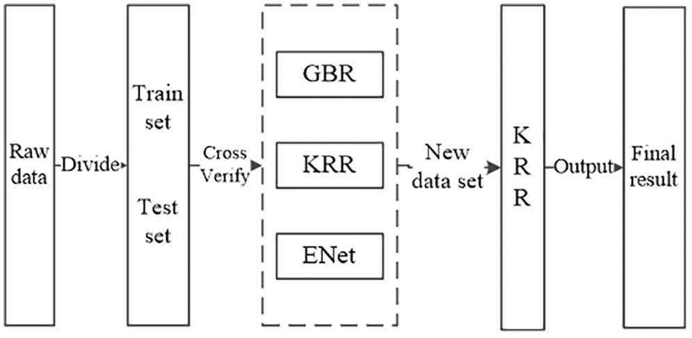
Figure 1: Stacking algorithm flow

Fig. 2 shows the K-fold cross-validation and model fusion part. It learns N models, each model is repeated k times, and uses the remaining k-1 groups as the training set to obtain a set of new prediction features. The model generates N groups of new features to shape a new training set. The new test data predicts the mean value of the original test set after the same number of times, and the final sample set constitutes a new sample set of the secondary learner.

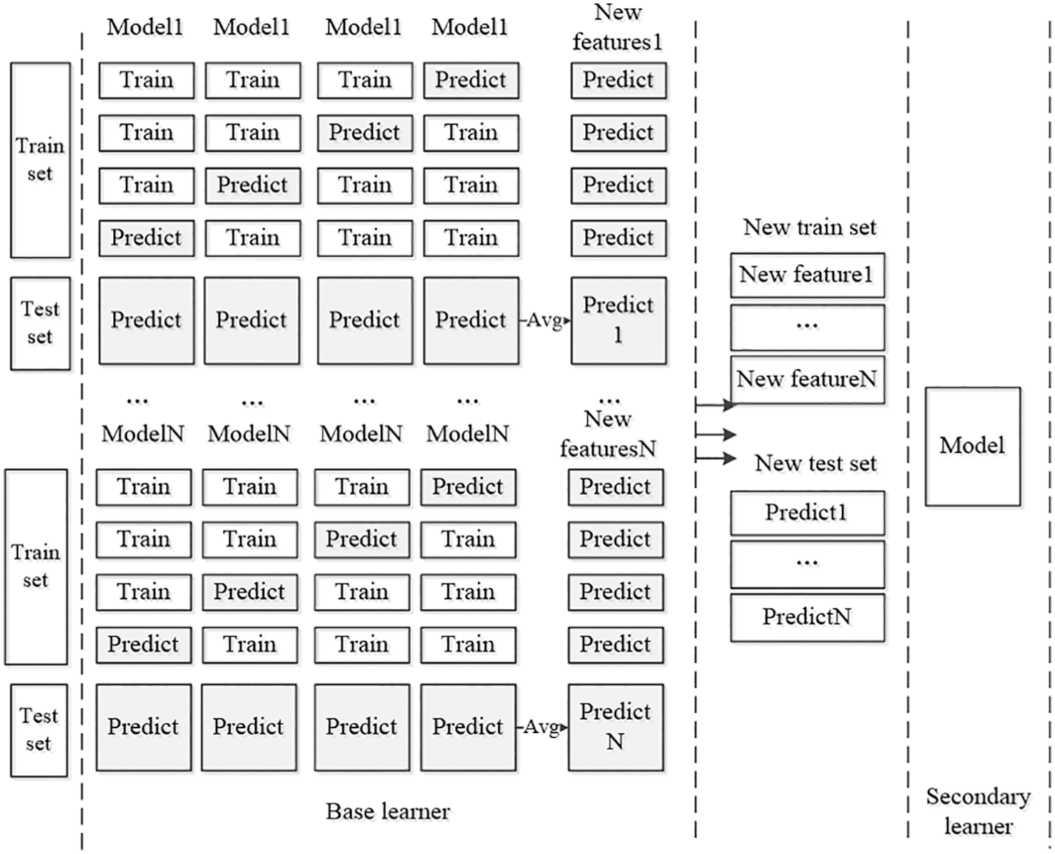
Figure 2: K-fold cross-validation and model fusion

3.2 Long Short-Term Memory Neural Network

LSTM effectively predicts the correlation of sequential signal data by learning the data storage information. The hidden layer contains three gating units for updating historical information: the structure of the input gate, and we show the gate control unit in Fig. 3.

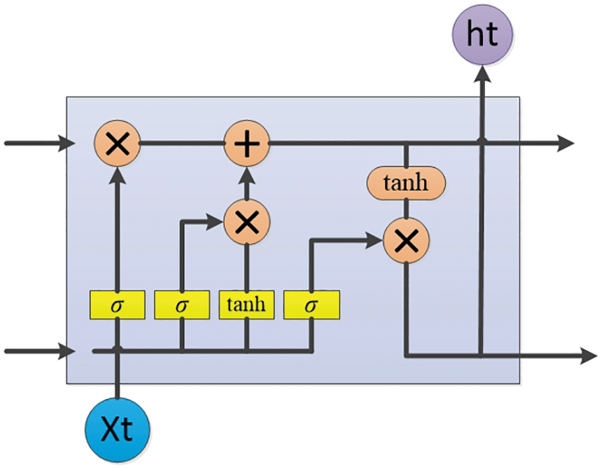
Figure 3: LSTM structure diagram

The input gate first screens the information input from the input layer at each moment, σ is the gate control unit, and the gate control unit at time t is as follows by Eqs. (16) and (17), equations are supported by reference [28]:

it=σ(wiht−1+wixt+bi)(16)

ft=σ(wfht−1+wfxt+bf)(17)

Cell memory state at time t is as follows by Eq. (18):

cellt=ft∗cellt−1+it∗tanh⁡(wcht−1+wcxt+bc)(18)

After the cell update state is known in the above, calculate the output gate o as:

ot=σ(woht−1+woxt+bo)(19)

ht=ot∗tanh⁡(cellt)(20)

In the equation, ht and ht−1 represent the external state, w and b are the learning parameters of the neural network, f and i are forget gate and input gate, and tanh is the activation function.

3.3 Stacking Model Fusion

The paper explains the architecture of the stacking model VMDPE-LSTM in Fig. 4.

Figure 4: Prediction process of VMDPE-LSTM

1)   Preprocess: fill the missing values with the mean of the neighbors of the outliers.

2)   Decomposition and reconstruction: in this paper, the final variable value K is used according to the center frequency value of the VMD algorithm, and the RMSE of the decomposed error is used as the indicator to select variable K. The permutation entropy algorithm estimates the intrinsic mode function’s complexity and reconstructs the components with similar entropy values and low complexity to reduce the difficulty of modeling.

3)   Component prediction: the LSTM network model predicted the reconstructed components and sub-sequences. Sliding window processes the residual component to obtain a sequence sample set with several samples and a time step of t. We use the sampled data of the first time point t as feature vectors and predict the next time point as a label.

4)   Reconstruct the final forecast: reconstruct the final forecast for analysis.

4  Results and Analysis

This article uses the public data set of Amazon cloud service of the public Kaggle platform, which contains 18050 pieces of data in about 2 months. The average CPU usage data set is a cluster data sampling period of 5 min and uses the average value of the adjacent values to fill in the missing values in the original data set.

4.1 Experimental Setup and Results Performance Comparison

1) Variational Mode Decomposition

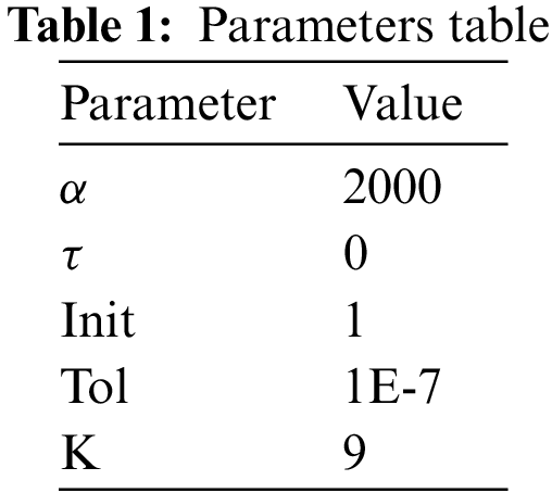
Compared with empirical mode decomposition, VMD does not need to pre-set the number of sub-modes. In this paper, the RMSE of the decomposed error is used as the indicator to select K. In addition to the decomposed modal number K, there are a large number of empirical values of other references for referencing. When K = 2, 3, 4, and 5 the original data is not completely stabilized. When K is 6–9, the RMSE is 2.03, 1.94, 2.41, and 1.43. At this time, when K is 9, the RMSE evaluation index results are the best. In the experiment, parameters such as penalty factor α, noise tolerance τ, initialization center frequency init, and convergence criterion tolerance tol are represented in Table 1, the parameters are supported by empirical values from reference [24].

After decomposition, Fig. 5 shows each component IMF1-9. The decomposed sub-modal components show apparent regularity, each component has obvious periodicity. There is no sharp random change, and the component data is stable for subsequent model prediction.

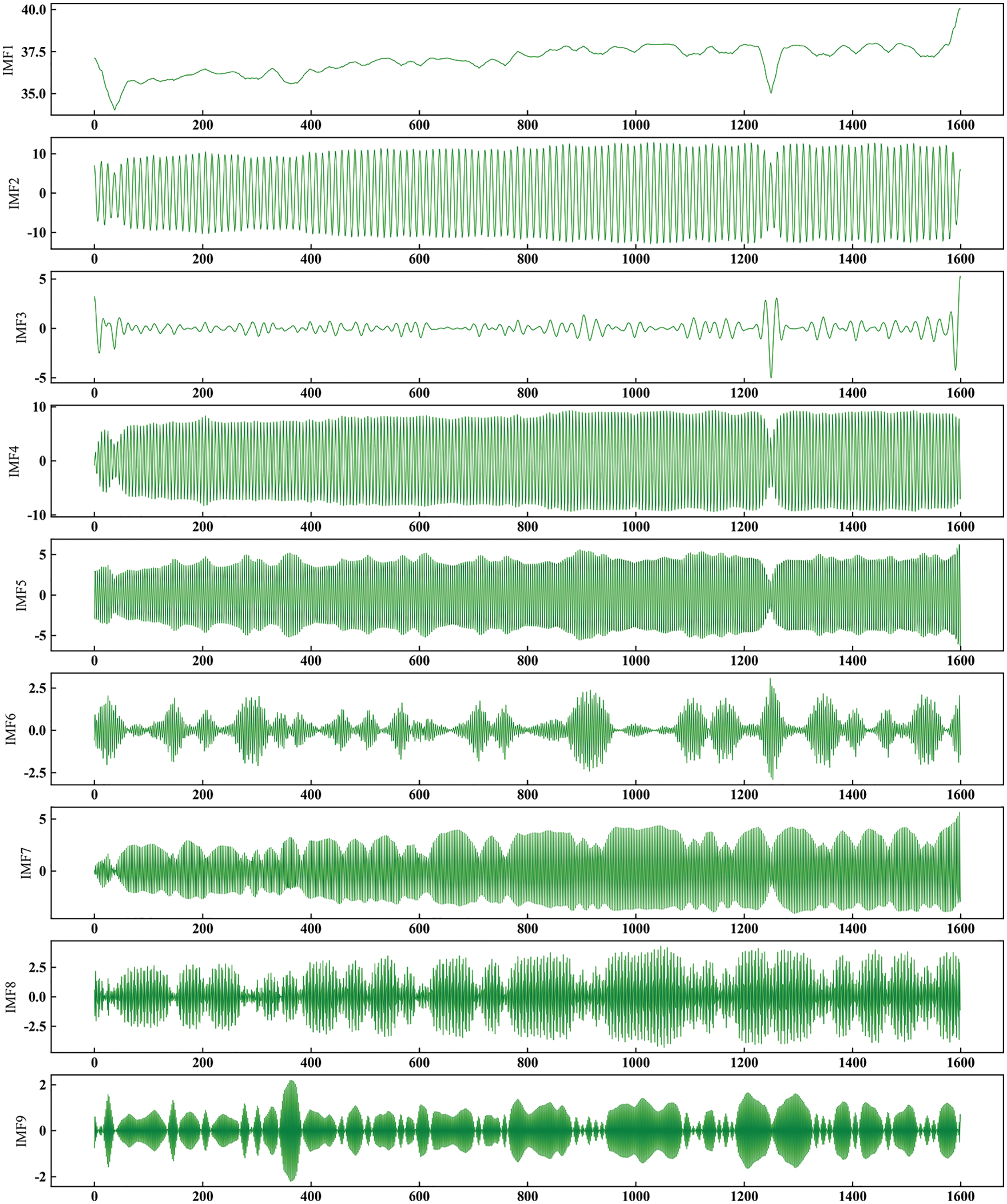
Figure 5: Submodel component

Fig. 6 shows the spectrum after component normalization. As shown in Fig. 6, each modal component has a single center frequency, the center frequencies of the decomposed modal components are evenly distributed in the frequency range, and no modal aliasing occurs. Fig. 7 shows the residual component, the residual component has no obvious periodicity, and the random fluctuation is large.

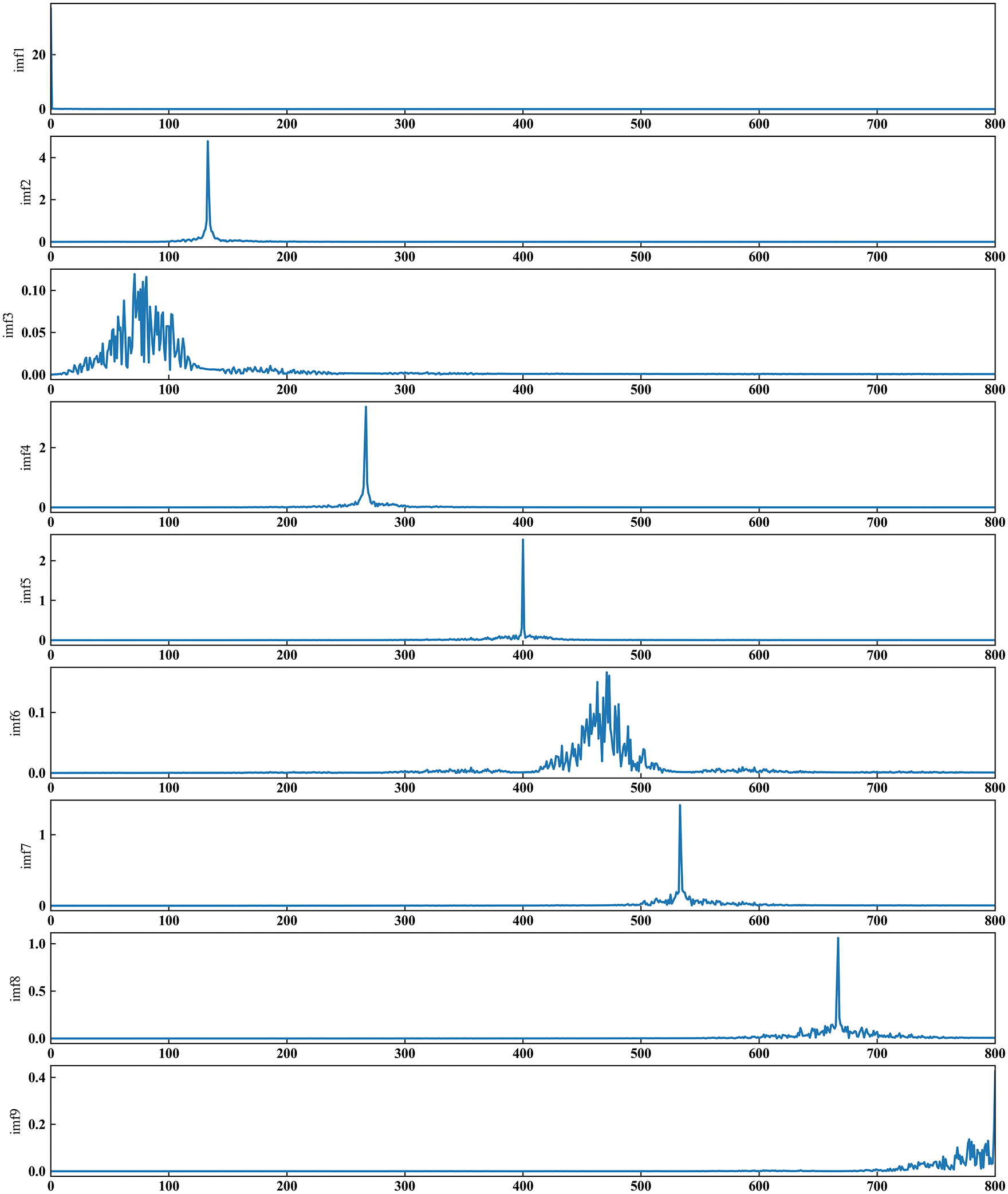
Figure 6: Amplitude spectrum after standardization

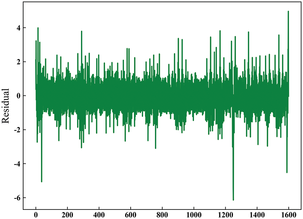
Figure 7: Residual component

2) Permutation entropy

The sub-modal complexity after variational modal decomposition is calculated by permutation entropy. Considering the high sensitivity of displacement entropy to change in time series data and the advantages of computational efficiency, we take it as the standard to evaluate the complexity of intrinsic mode function and reconstruct components with similar entropy values and low complexity to reduce the difficulty of modeling. Fig. 8 shows the arrangement entropy value of each subsequence component.

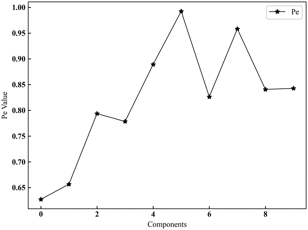
Figure 8: Submodel permutation entropy

As shown in Fig. 8, the permutation entropy values of subsequences IMF1-4 are all less than 0.8. While the permutation entropy values of IMF5-9 and residual component IMF10 are both above 0.8 and close to the original data permutation entropy value of 0.94, indicating that IMF5-10 subsequence noise. There is much interference and complexity. To avoid affecting the prediction accuracy, we only recombine the subsequences IMF1-4.

3) Model integration

First, the reconstructed word sequence is predicted by the long short-term memory network, the RMSE can evaluate intrinsic mode function, and the prediction errors of reconstructed component 1 and sub-modalities IMF5-9 are 0.4823, 0.339, 0.220, 0.269, and 0.106. The prediction error of the residual component R is 0.779, which is much larger than that of each sub-modal. In order to avoid affecting the overall prediction results, we use the stacking model fusion technology with strong generalization ability to increase poor prediction accuracy caused by unbalanced residual samples and finally reconstruct the subsequence prediction results.

Moreover, Fig. 9 shows the residual component IMF10 prediction result, and Fig. 10 shows the subsequence prediction results after reconstruction.

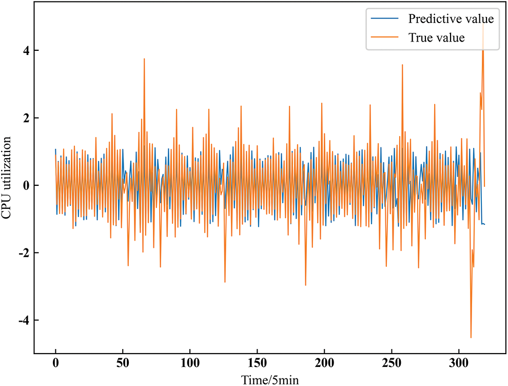
Figure 9: Residual component 10 predictive value

Figure 10: Submodel component prediction

Fig. 10 shows that the sub-components show a seasonal and periodic change, the original data and the predicted values are well-fitted, there is no significant fluctuation error, and only a tiny error occurs at the peak. However, as shown in Fig. 9, the residual component IMF10 has large randomness and volatility, and the fluctuation at the peak is significant. However, its prediction result has a better fitting effect at the concentration.

The linear prediction method Holt-Winters, the LSTM neural network method, and the sequential data integrated prediction model NeuralProphet [29,30] method are compared with the VMDPE-LSTM integrated model in this paper. We can see the performance effect comparison of each model in Fig. 11.

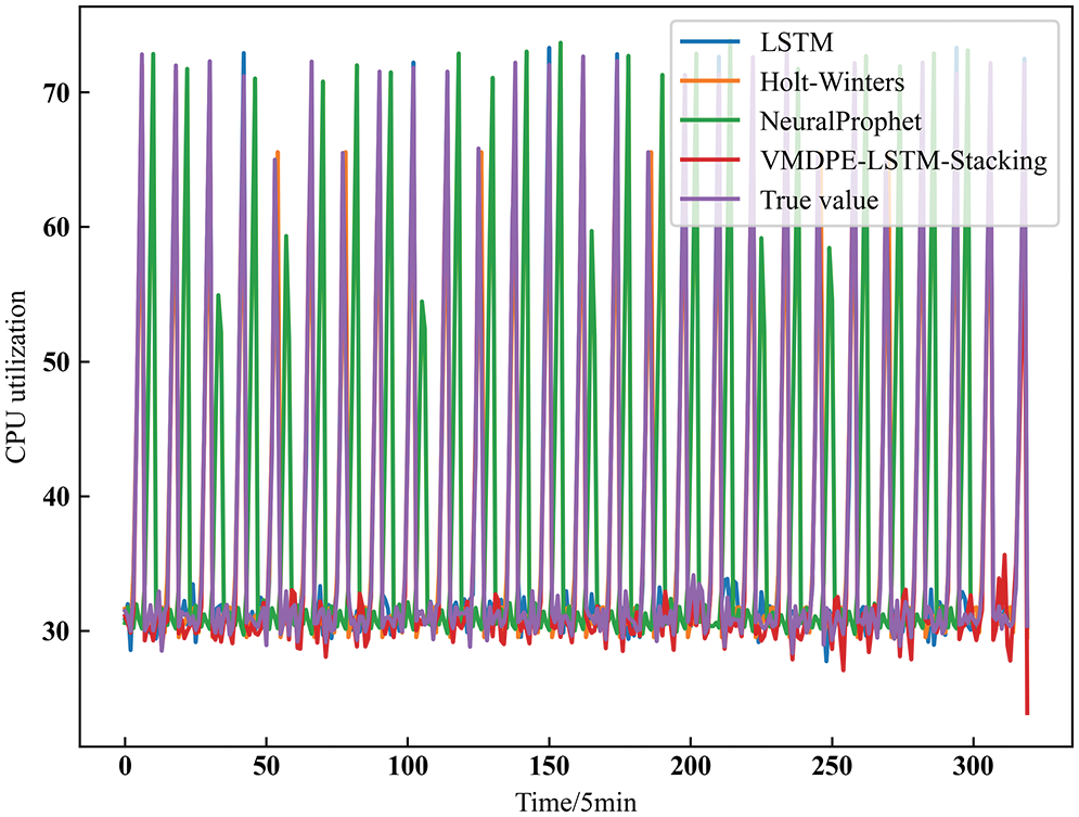
Figure 11: Model performance comparison

From the model performance comparison in Fig. 11 above, we can see that the VMDPE-LSTM integrated prediction model can better fit the actual data, the overall error is small, and the prediction trend more stably follows the periodic change of the actual value. Only obvious errors occur at the peak fluctuations. Compared with the Holt-Winters, LSTM, and NeuralProphet prediction models, the model in this paper can be closer to the actual value, and the prediction accuracy and stability are better. Since the decomposed sub-modal and residual components are more stable than the original data, the prediction and integration of the components have absorbed the advantages of each model and improved all aspects. The specific numerical performance is shown in Table 2 and Fig. 12.

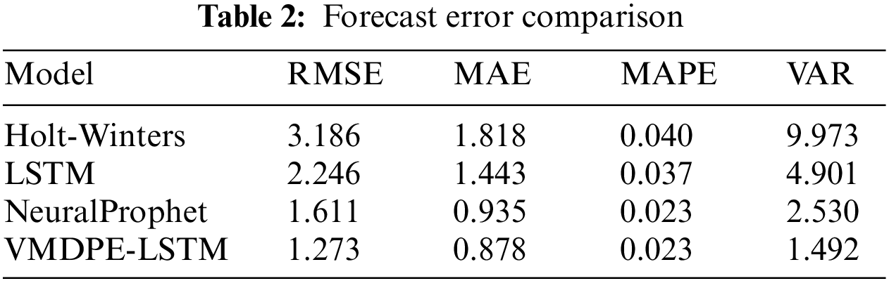
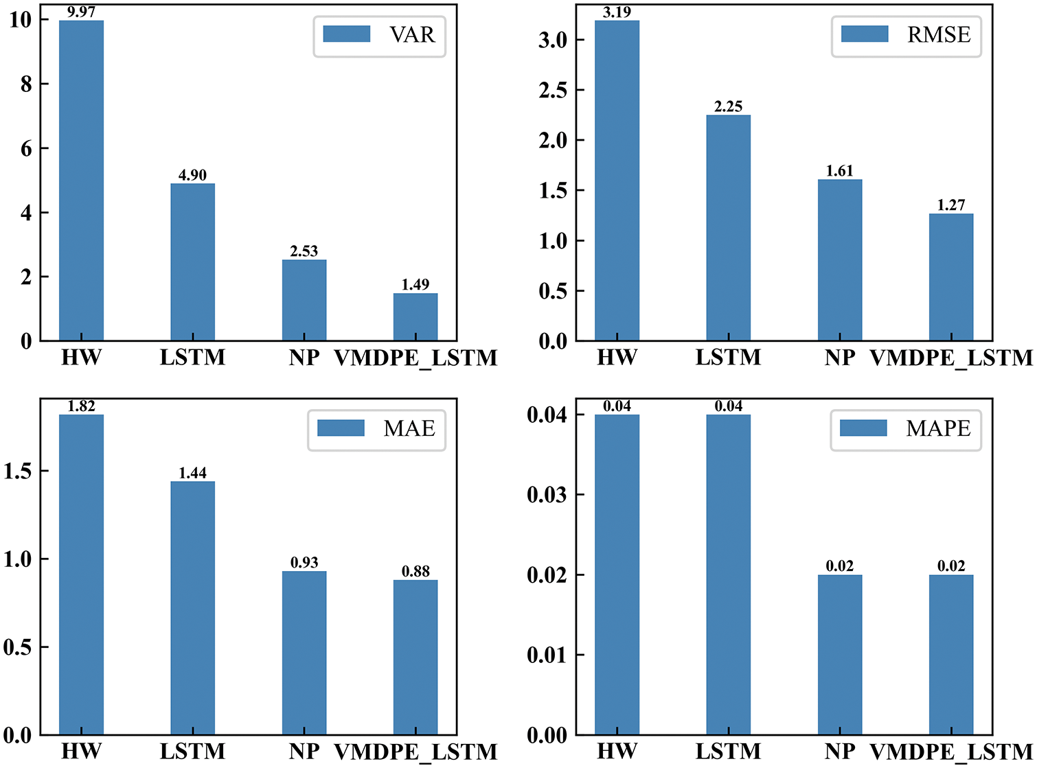
Figure 12: Prediction residual histogram

4.2 Experimental Error Comparison

1) Evaluation indicators

To explain the effect of the experimental error, we use four prediction performance indicators to compare. The variance indicator is an index to analyze and judge the stability of the model.

The root means square error equation:

RMSE=1n∑t=1n(yt∗−yt)2(21)

The mean absolute error equation:

MAE=1n∑t=1n|yt∗−yt|(22)

The mean absolute percentage error equation:

MAPE=1n∑t=1n|yt∗−ytyt|(23)

The variance D(n) is used as the degree of data fluctuation to judge the stability of the result, expressed by VAR, and r is the residual between the prediction and the actual value:

D(n)=[∑i=1n(|r−r¯|)2]/n(24)

In the equations, yt is the value of the original data set, y*t is the model predicted value, n is the data length, and the formula result is inversely proportional to the prediction effect.

2) Analysis and comparison of results

Table 2 is a comparison chart of prediction residuals, and Fig. 12 is a histogram of prediction residuals. Table 2 shows the effect of model performance comparison in Fig. 12 numerically.

Holt-Winters and NeuralProphet in Fig. 12 are represented by their abbreviations HW and NP. This paper's VMDPE-LSTM integrated prediction model is 1.913, 0.940, 0.017, and 8.481 lower than Holt-Winters in evaluation indicators and 0.338, 0.057, 0.00, and 1.038 lower than NeuralProphet 0.973, 0.563, 0.014, and 3.409 lower than LSTM. The variance shows the better stability of the prediction model, and the error histogram clearly shows that the model in this paper is at the lowest point in all indicators, which has a better effect and significantly improves the model’s accuracy.

5  Summary

The paper mainly resolves the prediction difficulty caused by the non-stationarity and volatility of resource data, and provides a container cloud resource integration prediction method based on VMDPE-LSTM. Adaptive signal decomposition algorithm VMD solves the non-stationarity of container cloud resource data. Moreover, permutation entropy reconstructs sub-components to improve computing efficiency and mines long-term dependencies using a long-term memory network to predict the regular time series after decomposition. The stacking fusion model absorbs the advantages of many different models, uses K-fold cross-validation to solve the problem of residual sample imbalance, and finally reconstructs the sub-sequence prediction results. We use the Amazon container cloud data to confirm the accuracy and efficiency of the method in improving the prediction accuracy and stability. It helps us respond to the container cloud workload in advance and determine the amount of resources needed subsequently. Therefore, service providers can select appropriate physical servers for scheduling and allocation to improve resource utilization and ensure quality of service. Then, this paper lacks relevant datasets to verify the adaptability of the method in this paper. While effectively planning container cloud resources, further research is needed to develop models with better adaptability and generalization capabilities. In the future work, the method in this paper should be applied to the actual container cloud physical machine, as well as extended to time series prediction in different fields to prove whether it is effective.

Funding Statement: The National Natural Science Foundation of China (No. 62262011), The Natural Science Foundation of Guangxi (No. 2021JJA170130).

Conflicts of Interest: The authors declare that they have no conflicts of interest to report regarding the present study.

References

1. S. N. S. Aasim and A. Mohapatra, “Repeated wavelet transform based ARIMA model for very short-term wind speed forecasting,” Renewable Energy, vol. 136, no. 1, pp. 758–768, 2019. [Google Scholar]

2. H. A. Li, M. Zhang, K. P. Yu, J. Zhang, Q. Z. Hua et al., “Combined forecasting model of cloud computing resource load for energy-efficient IoT system,” IEEE Access, vol. 7, pp. 149542–149553, 2019. [Google Scholar]

3. Y. Xie, M. P. Jin, Z. P. Zou, G. M. Xu, D. Feng et al., “Real-time prediction of docker container resource load based on a hybrid model of ARIMA and triple exponential smoothing,” IEEE Transactions on Cloud Computing, vol. 10, no. 2, pp. 1386–1401, 2022. [Google Scholar]

4. G. Dudek, P. Pełka and S. Smyl, “A hybrid residual dilated LSTM and exponential smoothing model for midterm electric load forecasting,” IEEE Transactions on Neural Networks and Learning Systems, vol. 33, no. 7, pp. 2879–2891, 2022. [Google Scholar] [PubMed]

5. M. C. Hsieh, A. Giloni and C. Hurvich, “The propagation and identification of ARMA demand under simple exponential smoothing: Forecasting expertise and information sharing,” IMA Journal of Management Mathematics, vol. 31, no. 1, pp. 307–344, 2019. [Google Scholar]

6. D. S. Wu, C. L. Zhang and J. Chen, “Improved LSTM neural network stock index forecast analysis based on genetic algorithm,” Application Research of Computers, vol. S1, no. 1, pp. 86-87+107, 2020. [Google Scholar]

7. W. Liu, X. Yu, Q. Zhao, G. Cheng, X. Hou et al., “Time series forecasting fusion network model based on prophet and improved LSTM,” Computers, Materials & Continua, vol. 74, no. 2, pp. 3199–3219, 2023. [Google Scholar]

8. W. Q. Xu, H. Peng, X. Y. Zeng, F. Zhou, X. Y. Tian et al., “A hybrid modeling method based on linear AR and nonlinear DBN-AR model for time series forecasting,” Neural Processing Letters, vol. 54, no. 1, pp. 1–20, 2021. [Google Scholar]

9. I. K. Kim, W. Wang, Y. Qi and M. Humphrey, “Forecasting cloud application workloads with cloud insight for predictive resource management,” IEEE Transactions on Cloud Computing, vol. 10, no. 3, pp. 1848–1863, 2022. [Google Scholar]

10. A. Alrashidi and A. M. Qamar, “Data-driven load forecasting using machine learning and meteorological data,” Computer Systems Science and Engineering, vol. 44, no. 3, pp. 1973–1988, 2023. [Google Scholar]

11. D. Sami Khafaga, A. Ali Alhussan, E. M. El-kenawy, A. Ibrahim, S. H. Abd Elkhalik et al., “Improved prediction of metamaterial antenna bandwidth using adaptive optimization of LSTM,” Computers, Materials & Continua, vol. 73, no. 1, pp. 865–881, 2022. [Google Scholar]

12. J. Bi, H. T. Yuan, L. B. Zhang and J. Zhang, “SGW-SCN: An integrated machine learning approach for workload forecasting in geo-distributed cloud data centers,” Information Sciences, vol. 481, no. 12, pp. 57–68, 2018. [Google Scholar]

13. H. X. Zang, L. Fan, M. Guo, Z. N. Wei, G. Q. Sun et al., “Short-term wind power interval forecasting based on an EEMD-RT-RVM model,” Advances in Meteorology, vol. 2016, no. 1, pp. 1–10, 2016. [Google Scholar]

14. J. Chen and Y. L. Wang, “A resource demand prediction method based on EEMD in cloud computing,” Procedia Computer Science, vol. 131, no. 4, pp. 116–123, 2018. [Google Scholar]

15. J. Qian, M. Zhu, Y. Zhao and X. He, “Short-term wind speed prediction with a two-layer attention-based LSTM,” Computer Systems Science and Engineering, vol. 39, no. 2, pp. 197–209, 2021. [Google Scholar]

16. Y. Liu and D. Zou, “Multi-step-ahead host load prediction with VMD-BiGRU-ED in cloud computing,” in 2022 IEEE 6th Information Technology and Mechatronics Engineering Conf. (ITOEC), Chongqing, CQ, China, pp. 2046–2050, 2022. [Google Scholar]

17. Z. Guo, M. Liu, Y. Wang and H. Qin, “A new fault diagnosis classifier for rolling bearing united multi-scale permutation entropy optimize VMD and cuckoo search SVM,” IEEE Access, vol. 8, pp. 153610–153629, 2020. [Google Scholar]

18. X. Chen, Y. Yang, Z. Cui and J. Shen, “Wavelet denoising for the vibration signals of wind turbines based on variational mode decomposition and multiscale permutation entropy,” IEEE Access, vol. 8, pp. 40347–40356, 2020. [Google Scholar]

19. J. Li and Q. Li, “Medium term electricity load forecasting based on CEEMDAN-permutation entropy and ESN with leaky integrator neurons,” Electric Machines and Control, vol. 19, no. 8, pp. 70–80, 2015. [Google Scholar]

20. L. Nie, J. Zhang and M. Z. Hu, “Short-term traffic flow combination prediction based on CEEMDAN decomposition,” Computer Engineering and Applications, vol. 58, no. 11, pp. 279–286, 2022. [Google Scholar]

21. X. F. Li and X. L. Xie, “Cloud resource combination prediction model based on HW-LSTM,” Science Technology and Engineering, vol. 22, no. 13, pp. 5306–5311, 2022. [Google Scholar]

22. Y. P. Wen, Y. Wang, J. X. Liu, B. Q. Cao and Q. Fu, “CPU usage prediction for cloud resource provisioning based on deep belief network and particle swarm optimization,” Concurrency and Computation: Practice and Experience, vol. 32, no. 14, pp. e5730, 2020. [Google Scholar]

23. K. Valarmathi and S. Kanaga Suba Raja, “Resource utilization prediction technique in cloud using knowledge based ensemble random forest with LSTM model,” Concurrent Engineering, vol. 29, no. 4, pp. 396–404, 2021. [Google Scholar]

24. W. J. Shu, F. P. Zeng, G. Z. Chen, T. T. Lu and J. Y. Liu, “Cloud resource prediction based on variational mode decomposition and gated recurrent unit network,” Journal of Computer Applications, vol. 41, no. S2, pp. 159–164, 2021. [Google Scholar]

25. Z. Tan, J. Zhang, Y. He, Y. Zhang, G. Xiong et al., “Short-term load forecasting based on integration of SVR and stacking,” IEEE Access, vol. 8, pp. 227719–227728, 2020. [Google Scholar]

26. Y. Zhang, P. Han, D. F. Wang and S. R. Wang, “Short-term prediction of wind speed for wind farm based on variational mode decomposition and LSSVM model,” Acta Energiae Solaris Sinica, vol. 29, no. 7, pp. 1516, 2018. [Google Scholar]

27. L. Y. Zhao, Y. B. Liu, X. D. Shen, D. Y. Liu and S. Lv, “Short term wind power prediction model based on CEEMDAN and improved time convolution network,” Power System Protection and Control, vol. 50, no. 1, pp. 42–50, 2022. [Google Scholar]

28. P. Hoang Vuong, T. Tan Dat, T. Khoi Mai, P. Hoang Uyen and P. The Bao, “Stock-price forecasting based on XGBoost and LSTM,” Computer Systems Science and Engineering, vol. 40, no. 1, pp. 237–246, 2022. [Google Scholar]

29. A. V. R. Manuel, “A case study of NeuralProphet and nonlinear evaluation for high accuracy prediction in short-term forecasting in PV solar plant,” Heliyon, vol. 8, no. 9, pp. e10639, 2022. [Google Scholar]

30. S. Khurana, G. Sharma, N. Miglani, A. Singh, A. Alharbi et al., “An intelligent fine-tuned forecasting technique for COVID-19 prediction using Neuralprophet model,” Computers, Materials & Continua, vol. 71, no. 1, pp. 629–649, 2022. [Google Scholar]