Dimensionality Reduction Using Optimized Self-Organized Map Technique for Hyperspectral Image Classification

1  Introduction

Hyperspectral image contains rich spatial and spectral information. Analyzing information-rich hyperspectral images have prominent applications in various domains like mining, military, agriculture, etc. [1,2]. Reflectance spectrum of hyperspectral images can be used to detect the different viability of objects. However precise analysis of different spectrums through the naked eye is quite impossible. Thus, image processing algorithms are used to extract the essential features from the hyperspectral images. The fine spectral resolution of images is obtained through remote sensing sensors which utilize multiple adjacent narrow spectral bands to construct an HSI image [3]. Hyperspectral sensors generate wavelength bands in the visible and infrared spectra [4,5] and analyzing these spectral bands will provide target information in a better manner [6]. The HSI image pixels are composed of electromagnetic radiation bands [7] and hypercubes are used to represent the HSI in three dimensions. The spatial information is represented in the first two dimensions and the third dimension is used for representing the spectral information. The spatial information (x and y) and the spectral information (f) are represented as hypercube as x * y * f to represent all the data [8,9].

While the large spectrum dimensionality of HSI helps with pattern identification precision, the processing and analysis of such a large amount of data are hampered [10]. It is also frequent in Hyperspectral image analysis for numerous spectral bands to be correlated, which means that redundant information is being processed. Because of this, dimensionality reduction is a key stage in the processing of HSI [11]. A classifier’s performance can be severely affected if redundant data is not removed using dimensionality reduction. Thus, dimensionality reduction in HSI processing can reduce costs and irrelevant resource utilization while maintaining information quality [12]. Nonlinear and linear dimensional methods include Maximum Noise Fraction (MNF) method [13,14] for noise removal. While processing HSI spatially, recent supervised dimensionality reduction algorithms are focused on decreasing the data’s dimensionality. A dimensionality reduction can be achieved by utilizing local neighborhood information, such as Fisher’s LDA [15] and regularised model [16]. But the fundamental drawback of these approaches is the requirement for labeled data to reduce the dimensionality. For RS applications, unsupervised dimensionality reduction approaches have gained attention because of the lack of this information [17,18]. The lack of labeled examples is addressed by unsupervised dimensionality reduction methods, which aim to identify a different illustration of the data in a lower space. In this research study, initially, noises are removed using the DL technique, and then the pre-processed image is fed into SOM for dimensionality reduction. In the SOM, weight is updated by using the optimization model. The experiments are carried out on two publicly available datasets in terms of several metrics.

The remaining discussions are arranged in the following order. A brief literature analysis of existing research works is presented in Section 2. The proposed optimized dimensionality reduction model is presented in Section 3. Experimental results and discussion are presented in Section 4 and the conclusion is presented in Section 5.

2  Related Works

Various dimensionality reduction methods are evolved in recent times which support Hyperspectral image classification applications. The dimensionality reduction model presented in [19] presents a shape adaptive tensor factorization model which extracts the patch features to develop fourth-order tensors. Similarly, the latent features are extracted in the presented approach using the mode i-tensor matrix. The dimensionality-reduced features are processed through sparse multinomial logistic regression to attain better classification performances. The dimensionality reduction model presented in [20] presents a graph-based spatial and spectral scaling cut procedure that incorporates both spectral and spatial domain features. The presented approach initially includes a guided filter to smoothen the pixels. Followed by smoothening, the local scaling cut procedure is employed to define the dissimilarities in features. A compressive dimensionality reduction procedure presented in [21] includes an optimized slice sparse coding tensor to reduce the high dimensionality of features. The dimensional reduced sparse features are classified using a tensor-based classifier to attain accurate classification performance with minimum computation cost.

An unsupervised method was presented in [22] for effective dimensionality reduction and classification of HSI images. The presented local neighborhood structure preserving embedding method reconstructs the samples based on neighbor spectral weights. The optimal weights are obtained from the reconstructed samples which are further used to develop adjacency graphs. The modification performed in the loss function greatly reduces the scatters and improves the classification performances compared to existing methodologies. The dimensionality reduction model for a Hyperspectral image incorporates a graph-based approach for effective dimensional reduction [23]. The presented multigraph embedding procedure initially captures the local and spatial information to develop a tensor subgraph. Then a bipartite graph is developed based on the relationship between the pixels and patch tensors. Finally, the deviations in the pixels are removed from the patch tensor and a pixel-based subgraph was developed to obtain the geometrical structures.

Researchers from Zhang et al. [24] developed an attention-based hierarchical homogeneity-based network to streamline computing by minimizing the number of comparable operations. According to CNN visual invariance, alterations to input images can have a significant impact on network performance. It has been proposed by Sabour et al. [25] to combine spectral–spatial feature extraction. Network robustness can be improved and more efficient position information can be preserved by using a capsule network (CapsNet), which was proposed in [26]. The DC-CapsNet has been introduced in 3D convolution by the author from [27] to improve the robustness of the learned spectral–spatial properties. CapsNet’s lack of labeled samples has recently been alleviated by GAN, which has shown satisfactory results. On the other hand, it has a difficult time modeling and preserving the relative locations of features [28]. The development of DL-based algorithms has also revealed several difficult problems. It has become increasingly challenging to deploy deep learning models on edge devices because of the increasing complexity of the model and the need for training samples and depths.

A general multimodal deep learning model is presented by Wu et al. [29] for remote sensory image classification. The presented fusion architecture performs pixel-wise classification considering the spatial information using a convolutional neural network. Experimentations provide better performance in remote sensory image classification compared to traditional approaches. A similar convolutional neural network-based remote sensing data classification model reported by Hong et al. [30] presents an advanced cross-channel reconstruction model using CNN. The presented approach provides compact fusion representations using reconstruction strategies and exchanges the information in an effective manner to obtain better classification performances. A semi-supervised 3D CNN (SS-3DCNN) was presented in a study [31] for the categorization of HSI. Using labeled and unlabelled training samples, this approach aims to overcome the problem of low training sample numbers and the “curse of dimensionality.” SS-3DCNN is utilized for HSI categorization once the specified bands have been input into them for processing. To classify HSI images, Zhang et al. [32] suggested a deformable convolution network for spectral–spatial attention fusion as SSAF-DCR. To advance the classification presentation of the HSI, the proposed model includes both feature classification networks. A 3D CNN is used to extract the HSIs’ spectral and low-level spatial properties, whereas a 2D CNN is used to recover the HSIs’ high-level spatial data. The SSAF-DCR strategy proved to be beneficial. For Hyperspectral image categorization, another study [33] presented a deep spectral-spatial inverted residuals network (DSSIRNet). To avoid the lack of labeled samples, DSSIRNet presented a data block random erasing technique. The DIR module for spectral bands is also projected in this paper. A 3D consideration module is also implemented and integrated into the DIR component.

Luo et al. [34] tried to remove the HSI mixed noise by spatial-spectral constrained deep image prior (S2DIP). Without any training data, the proposed model removed the noise by using hand-crafted priors. The DIP-based model’s semi-convergence behavior is avoided by the proposed model. An algorithm called the alternating direction multiplier model is used to enhance the denoising ability of the DIP model. Zeng et al. [35] removed the HSI mixed noise by proposing nonlocal block-term decomposition (NLBTD). Global spectral and non-local self-similarity features are captured by using BTD for preserving the smoothness of local spectra. Based on the proximal alternating minimization, the mixed noises in HSI are removed to increase the efficiency of NLBTD. Wang et al. [36] improved the strip removal and avoided the poor generalization ability by proposing Translution-SNet. The proposed model is used to remove the strip noise of HSI by applying the convolution and transformer as feature extraction. The loss function from noisy data is calculated by using an unbiased estimation method. During strip removal, various complex stripe noises are dealt with through semi-supervised methods to improve the Translution-SNet.

3  Proposed Methodology

3.1 Noise Reduction Using the Proposed DL Model

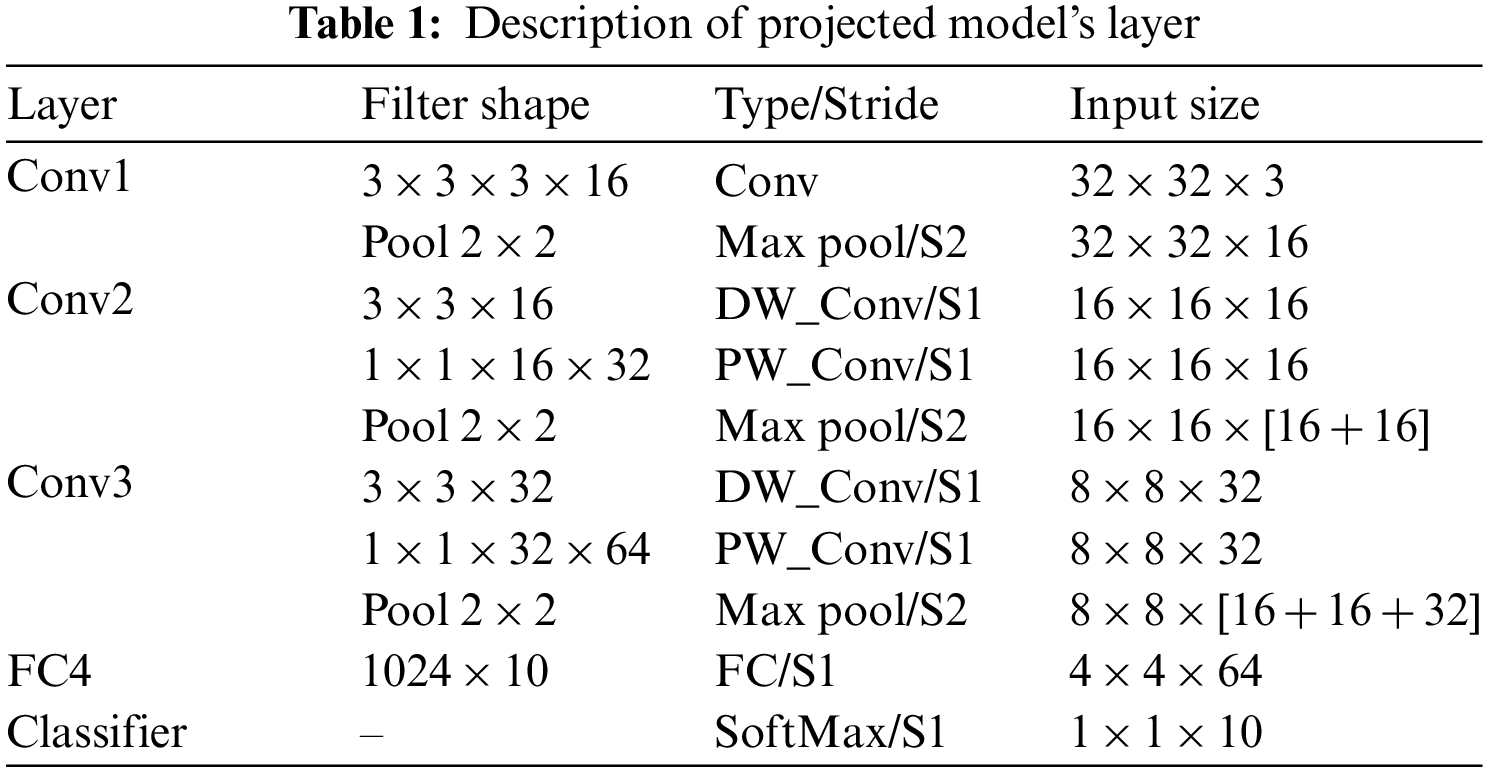
In all individual matrices representing the input image, there are equivalent kernel matrices and biases. Finally, activation functions for all individual pieces have been developed. Behind the Back-Propagation (BP) phase, feature detection filters are constructed by altering bias and weight values. A feature map filter is applied to each of the three channels to minimize the amount of noise in the images that are being processed. Using a technique called “pooling layers,” CNN reduces the amount of data it needs to work with to reduce the amount of noise it has to deal with in its final output. To protect the crucial features, the usual pooling methods are used. The max-pooling method is one of the most well-known methods of pooling, and it involves selecting the largest activation in the pooling window. Using sigmoid (Eq. (1)) or ReLU (rectified linear activation unit) (Eq. (2)) activation functions, CNN has applied a BP approach to perform a discriminative function. According to Eq. (3), the final layer has one node that has a beginning function for binary classification and another node that has an activation function for multi-class issues [37].

f(x)=11+e−x∈(0,1)(1)

f(x)=max(0,x)(2)

σ(z)j=ezi∑k=1Kezk∀j∈{1,…,k}(3)

For image categorization, the DWS convolutions were used. It is a type of factorized convolutional that breaks down depth-wise convolutions. With only one filter per input channel, the depth-wise convolutional filtering (Fig. 1) performs lightweight filtering. Next, the input channels are combined in a linear fashion using a point-wise convolution [30]. Standard convolutional functions are returned by using DWS convolution, which returns a factorized 2-layer convolution and a single layer to space filter. It is therefore possible to reduce computation/noises of the input images and mode size by using depth-wise separable convolutional. The standard convolution layer receives a feature map of h×w×cin input I and performs a k×k× cin × cout  convolution kernel K to yield an output feature map O by using h×w×cout where h and w are the input feature map dimensions, k is the square kernel spatial dimension, cin is the input channel count, and cout is the result channel count. The output feature map can be assumed to have the same spatial dimensions as the input feature maps because of the zero-padding meaning. A normal convolutional is characterized by a difficulty in computation (the function counts). Table 1 shows the architecture layer description of the projected model.

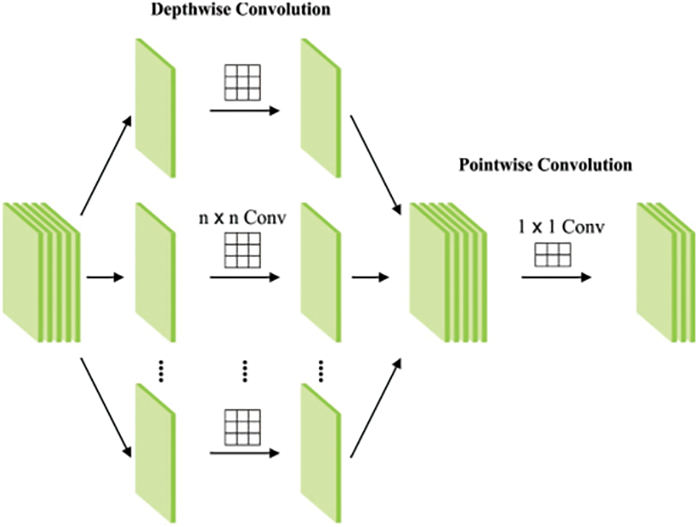
Figure 1: Structure of proposed depth-wise CNN

All of the separable convolutional parts can be separated. It uses depth-wise convolutional filtering to apply a single filter to all input feature maps, which is given in Eq. (4).

G(y,x,j)=∑u=1k∑u=1kK(u,u,j)×I(y+u−1,x+u−1,j)(4)

in which K implies the kernels of size k×k×cin. The nth filter is used to yield the nth channel of the filtered result feature map G, K is functional to the I channel. To determine the linear group of depth-wise results when constructing new features, a point-wise convolutional requires 11 convolutions. Point-wise convolutions can be expressed using the formula in Eq. (5).

0(y,x,I)=∑j=1cinG(y,x,j)×P(j,l)(5)

1×1  Convolutional kernel has a size of 1×1×cin×cout. It is possible to change the feature map by changing m. There are no restrictions on the locality of dense 1×1 convolutional functions like those found in other convolutional functions; hence there is no need to re-arrange the parameters in memory. Then, using incredibly efficient matrix multiplication algorithms, it is carried out immediately. It is difficult to express a convolutional calculation as shown in Eq. (6).

Cds=k2⋅cin⋅h⋅w+cin⋅cout⋅h⋅w(6)

The cost of depth-wise convolution and 1 × 1 point-wise convolution is shown below. A DWS convolutional is related to the normal convolutional in that it reduces the calculation difficulty by a factor as shown in (7).

η=CdsCstd=k2cinhw+cincouthwk2cincouthw=1cin+1k2(7)

The factor is roughly comparable to 1k2 because the value of m is typically very large. As a result of using 3×3 DWS convolutional layers in this research, the calculation complexity and parameter count of layers are 7∼8 times lower than with regular convolutions.

3.2 Dimensionality Reduction Using Proposed Optimized SOM

An approach based on maps to reduce the size of an HSI is presented in this section. As a first step, the image is reduced to a lower dimension using the dimensional reduction approach projected in this study and based on optimized SOM. The use of optimized SOM is to reduce the spatial dimensions of hyperspectral image (HSI). SOMs are inspired by the human brain’s ability to focus on the most important aspects of the universe. Using self-organized maps, high-dimensional data in HSI can be grouped. This type of network has only one input and one output layer, and there are no hidden layers. Relationships within the input patterns are automatically discovered by the SOM network. To solve the difficulty of mapping images from higher to two-D feature space for image cataloging, this property can be employed. A SOM network is defined by the neurons in the input and output layers. Each feature has the same amount of input neurons. The output layer of a SOM is typically a two-dimensional layer with M×M neurons. The synaptic weights wij connect the neurons in the input and output layers, where i, and, j represent neurons’ unique identities, respectively. During training, the weights are arbitrarily assigned and then fine-tuned by using the Water Strider Optimization algorithm (WSOA) to better arrange the relationships between the input patterns. The WSOA is a nature-inspired population-based optimizer that is inspired based on the life cycle of water strider bugs. The optimization model is framed by characteristics of the bug’s insect succession, territorial behavior, feeding mechanisms, mating style, and clever ripple communication [38]. In the next sections, we go over the basics of this strategy.

3.2.1 Initial Birth

Here’s how the search space is filled with the possible solutions/water striders (WS):

WSi0=Lb+rand, (Ub−Lb);i=1,2,…nws(8)

If WSi0 represents the initial weight of ith WS in the lake/SOM. The lower and upper boundaries are denoted by Lb, and, Ub, respectively. An arbitrary number between zeros and ones and the number of WSs is denoted by rand (population size). Based on objective functions, the first position of WSs is determined.

3.2.2 Territory Establishment

Based on an individual’s level of fitness, the WSs are organized and the nws/nt number of groups are formed in order. For each group, the j-th member is given an equal number of territories, which range from  1 tont. As a result, the total sum of WSs in each territory is equal to nws/nt. The sites with the best and worst fitness are assigned to men and women, accordingly (keystone).

3.2.3 Mating

To mate, the male WS sends out a ripple signal to the female. The likelihood of attraction or repulsion is calculated based on the fact that the behavior of females is unknown [39]. p is always set to 0.5. These changes have been made to the location where the male WS can be found:

{WSit+1=WSit+R⋅rand;if mating happens (with a probability of p)WSit+1=WSit+R⋅(1+rand);otherwise.(9)

The length of R is projected as follows

R=WSFt−1−WSit−1(10)

where WSFt−1andWSit−1 signify the male and female WS in the (t−1)th cycle, reprehensively.

3.2.4 Feeding

The male water strider forages for food after mating, which requires a lot of energy for the water strider. Using Eq. (11), the male WS will seek out the lake’s best-suited WS to find prey.

WSit+1=WSit+2rand∗(WSBLt−WSit)(11)

3.2.5 Death and Succession

The male WS would die in the new site, and a new WS would take its place as follows:

WSit+1=Lbjt+rand∗(Ubjt−Lbjt)(12)

where Ubjt and Lbjt are the greatest and negligible values of WSs† situated inside the j-th territory.

3.2.6 WSOA Termination Criterion

For a novel loop, the process would return to the coupling stage if the end criteria were met. At this point, the supreme quantity of function evaluation or updated weight is taken into account as a final criterion. Final weights wij show how well the input features have been characterized once the training process is complete. Essentially, a multidimensional input space is predictable into a two-dimensional output space.

3.2.7 Training of Optimized SOM Model

Competitive learning is the SOM training philosophy. The neurons in the output layer must strive with one another to respond to the input pattern. It is so possible to adjust at once all the weights of M×M neurons. An adjustment is made to the weights of the winning neuron and its neighbors, but not the rest of the input layer.

Then, taking a Hyperspectral image X(N×p) where N=n×m is defined as Xi(p×1), which contains each spectral feature of the ith pixel. wij(M2×p) by multiplying each spectral input vector Xi(p×1) with the ith pixel’s respective nm-sized output vectors. These results generate output vectors with dimension M2 with an input vector Xi(p×1). The dimensionality of the self-organized map decreases as the map size grows. By utilizing an optimized self-organized map, a 1−M2=p dimensional reduction ratio can be obtained (13).

X^i(M2×1)=wij(M2×p)Xi(p×1)

%Reduction=1−M2p(13)

The proposed dimensional reduction method described in this study and based on self-organized maps is depicted in Algorithm 1.

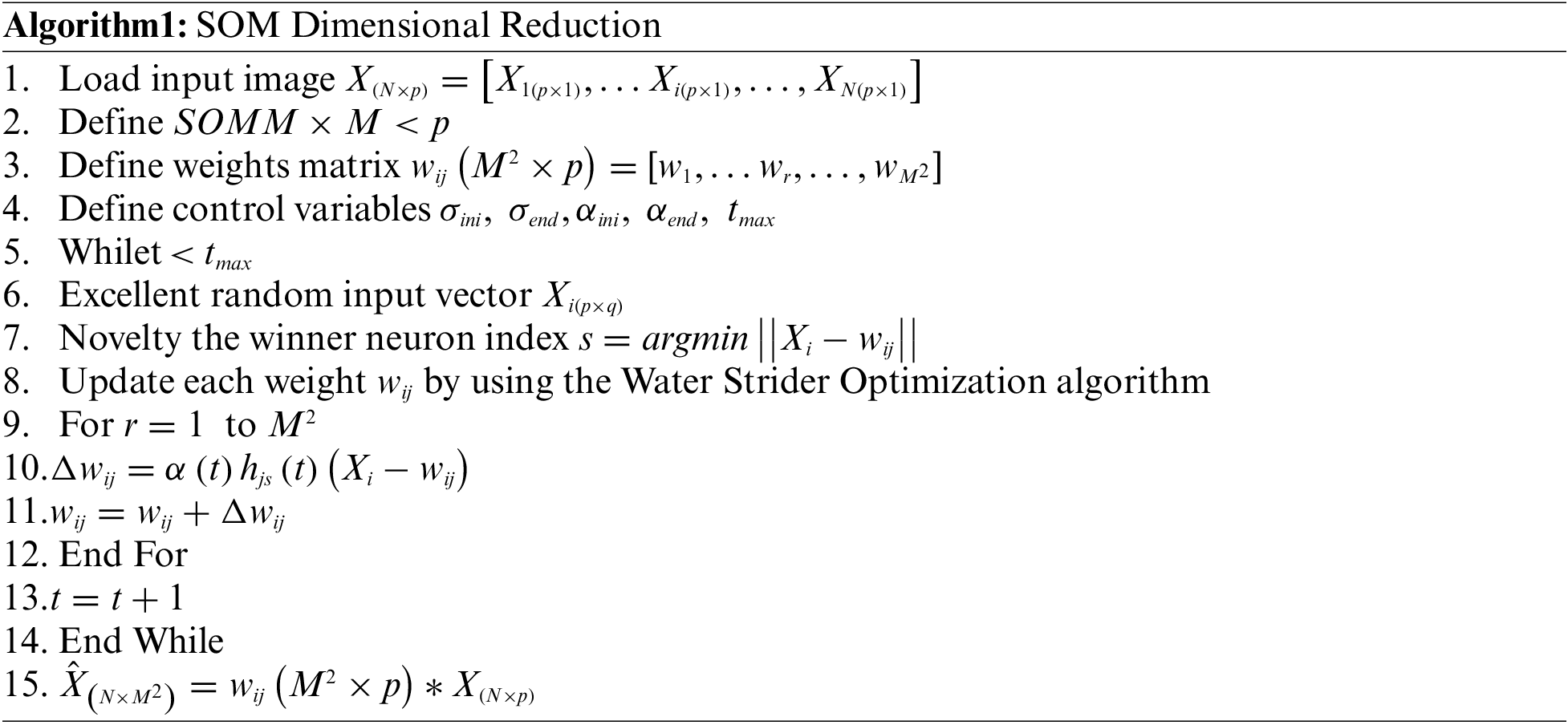
On lines 1 to 3, Algorithm 1 begins by loading X(N×p) and then creating a self-organized map with M neurons, wij(M2×p). There are many possible inputs to the iterative process, but the one used here is a randomly generated input vector Xi(p×1), and the final winner neuron location s will be determined by finding the vector wij with the lowest distance between each input and each of the associated weighting vectors (14).

s=argmin||Xi−wij||(14)

For the self-organizing map, Eq. (15) specifies how the synapse weights change over time, which includes the learning rate (t), each synapse weight wij and the iteration index (t).

Δwij=α(t)hjs(Xi−wij)(15)

tmax is the maximum sum of iterations that can be used in the training process, while αini and αend are the initial and final learning rates respectively. Eq. (16) seeks to have the neurons quickly adapt to the input data at the start of the training phase. The learning rate decreases as the procedure progress to achieve a better fit in training.

α(t)=αini(αendαini)tmax(16)

The neighborhood function hjs(t) is calculated using Eq. (17), It can be expressed as a Gaussian curve. The farther neuron is away from the winning neuron, the less influence it has on the other neurons.

hjs(t)=e(−d(js)22σ2ini(σend/σini)2tmax)(17)

where neurons sandr are separated by an angle of d; this changes the synaptic weights of neurons j. To ensure that the learning algorithm convergence is stable, the neighborhood variable rank r must be used.

The synaptic weights matrix wij(M2×p) is created at the end of the iterative process outlined above. As a result of this, an output matrix X^ with dimension n×m×M2 has been generated (line 15). In each application, the correct value of M is determined heuristically. After the previous operation, a data subset with n×m pixels and M2 dimensions is obtained.

4  Results and Discussion

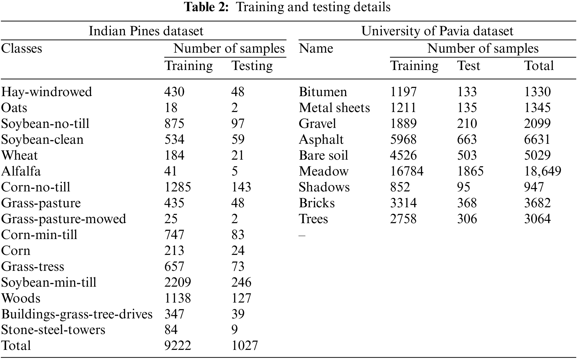
The proposed model experimental analysis includes two datasets as Indian Pines dataset and the University of Pavia dataset. The Airborne Visible and Infrared (AVIRIS) sensor captured the Indian Pines (IP) dataset, which was the starting point for this research work. Each class has a 145 × 145-pixel spatial resolution and 220 spectral bandwidths. It is further characterized by the removal of 104–108, 150–163, and 220. The spectral wavelength is between 0.4 and 2.5 micrometers. 10% of the samples from each class were used in the training, while the rest were used for testing. Table 2 lists the total number of training and testing samples for each class. As a second source, we turned to Italy’s University of Pavia dataset (UP), which was gathered using the ROSIS imaging spectrometer. It measures 610 × 340 pixels in width and height. After removing the noisy bands, it has 103 spectral bands, each with 200 training samples; the remaining samples were used for testing purposes. For each class, the numbers in Table 2 reflect how many training and testing samples were used.

4.1 Performance Validation of the Proposed Model

We have utilized an Intel Xeon W-2123 CPU with 64 GB of RAM and an NVIDIA GeForce GTX 2080 Ti GPU with 11 GB of RAM in the experimental configuration. The Pytorch 1.6.0 DL frameworks are used in conjunction with a 64-bit Windows 10 OS. In terms of overall accuracy (OA), average accuracy (AA), and Kappa coefficients, classification accuracy is measured.

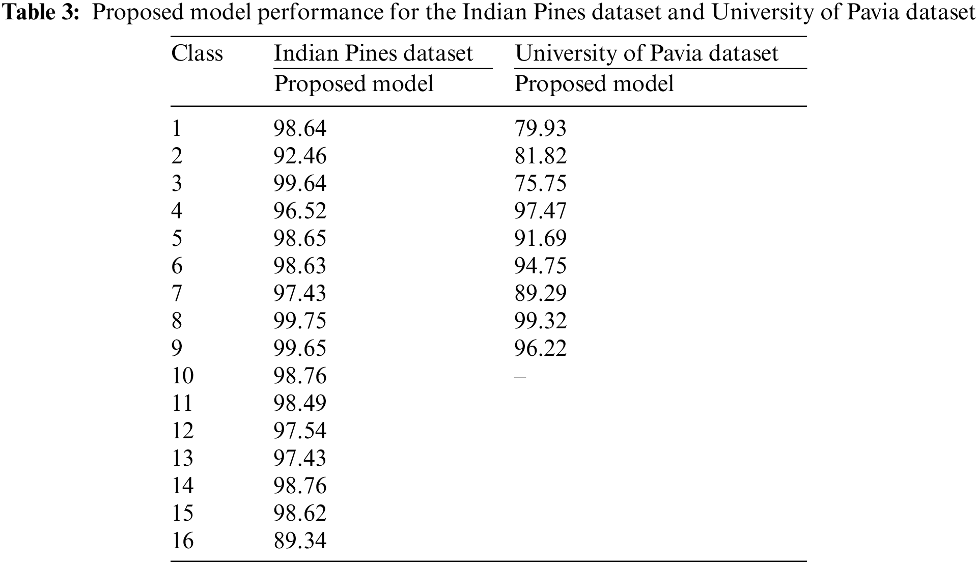
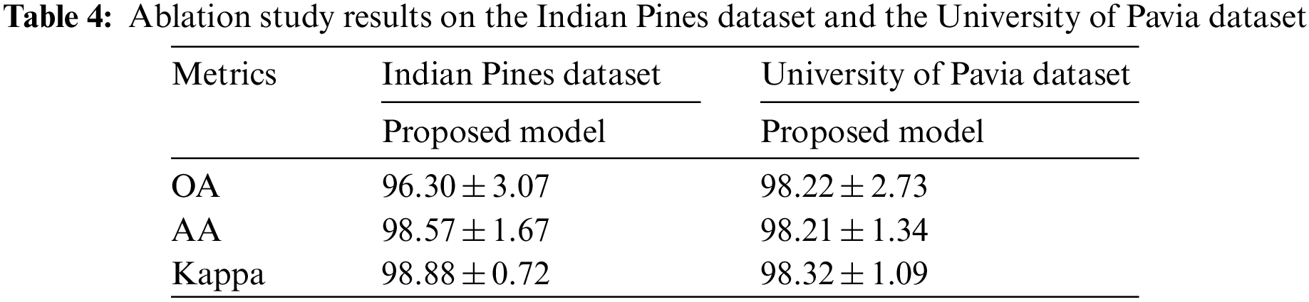
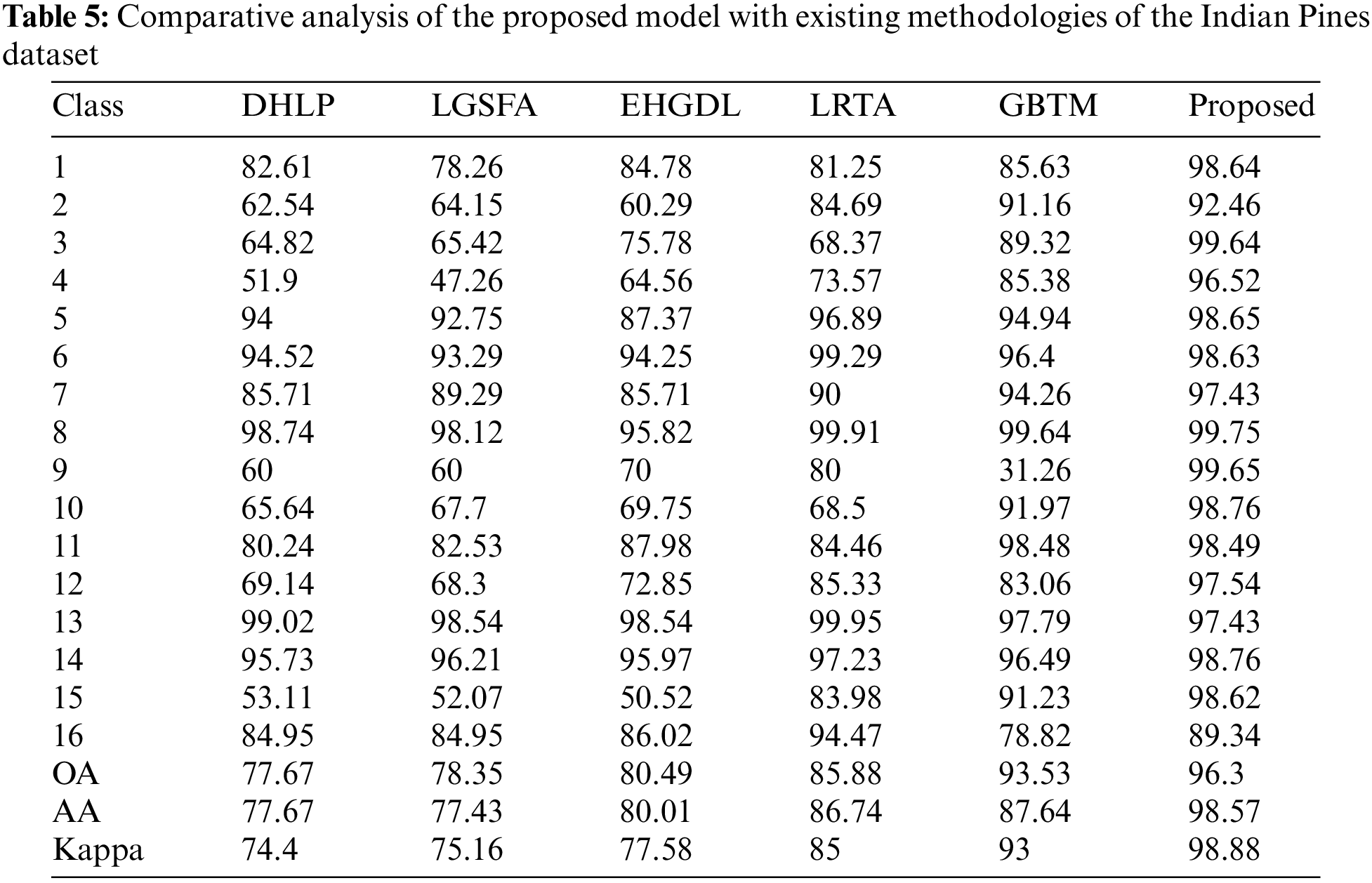
Further to validate the performance of the proposed model, different dimensionality reduction techniques are compared with the existing methods like Enhanced Hybrid-Graph Discriminant Learning (EHGDL), local geometric structure Fisher analysis (LGSFA), Discriminant hyper-Laplacian projection (DHLP), Group-based tensor model (GBTM), and Lower rank tensor approximation (LRTA) methods. The results are obtained from Luo et al. [40] and An et al. [41] research works that perform dimensionality reduction in Hyperspectral images. The dataset which was used in the proposed work was used in the existing methods so that the results are directly compared with the proposed model results given in Table 3. The ablation study results on the Indian Pines dataset and the University of Pavia dataset are given in Table 4, which describes the overall accuracy, average accuracy and Kappa coefficient of the proposed model. The following data given in Table 5 presents the comparative analysis of the proposed model and existing model performances for the Indian pine dataset. From the results, it can be observed that the performance of the proposed model is much better than the existing methods in terms of overall accuracy, average accuracy, and kappa coefficient.

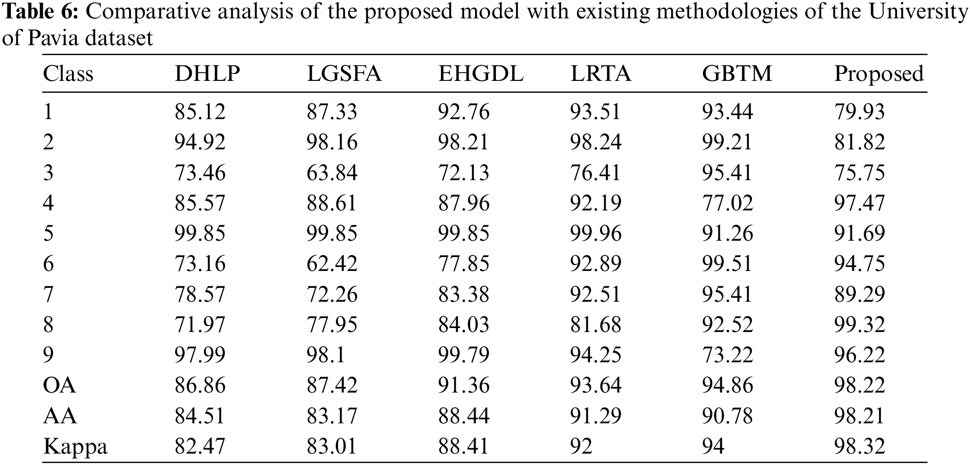
Similarly, the performance of the proposed model is compared with existing methods for the University of Pavia dataset. Table 6 depicts the performance comparative analysis and it can be observed from the results that the performance of the proposed model is much better than the existing methods.

Further to validate the impacts of dimensionality in the overall accuracy metric, different dimensional measures are employed and measured the overall accuracy for the proposed model. Fig. 2 depicts the performance comparative analysis of the proposed model and existing models for different dimension rates. The dimensionality is varied from the minimum on a scale of ten and measured for the maximum value of 100. Fig. 2 depicts the variations in the overall accuracy of the proposed and existing methods for the Indian Pines dataset. Similarly, Fig. 3 depicts the variations in the overall accuracy of the proposed method and existing methods for the University of Pavia dataset. Due to the maximum dimensional reduction without any feature loss proposed model attains maximum accuracy compared to other methods for both datasets.

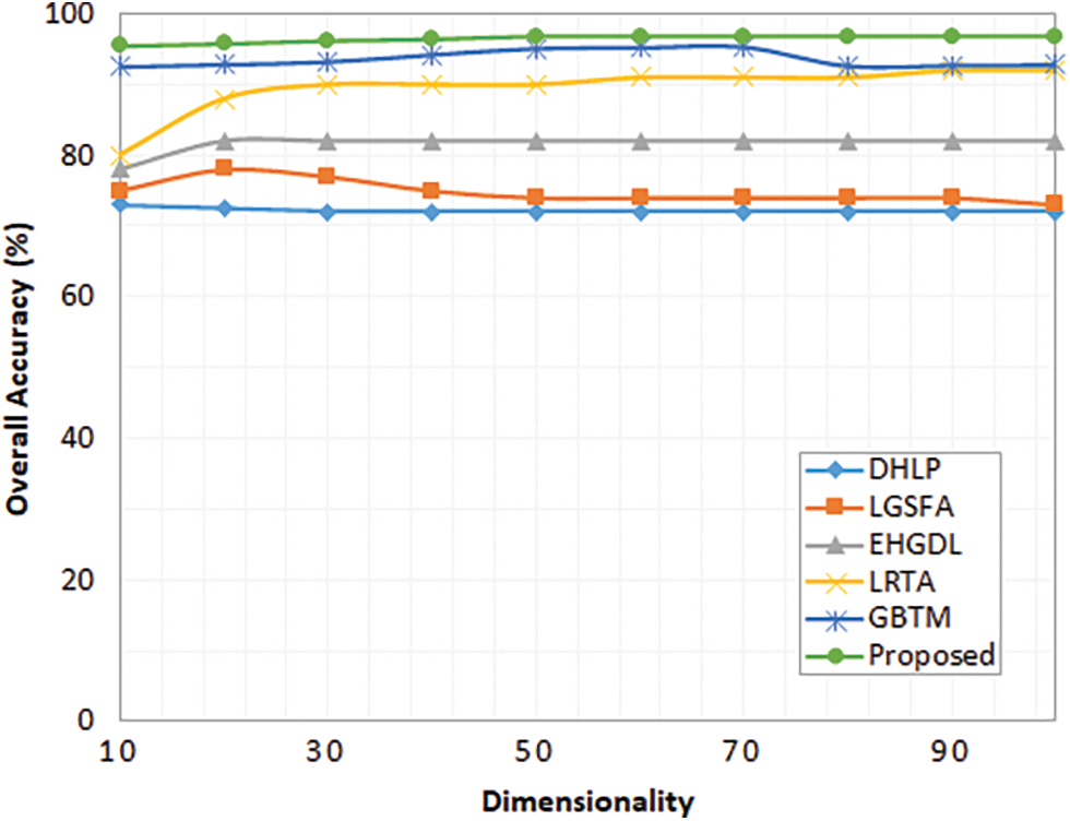
Figure 2: Overall accuracy for different dimensionalities (Indian Pines Dataset)

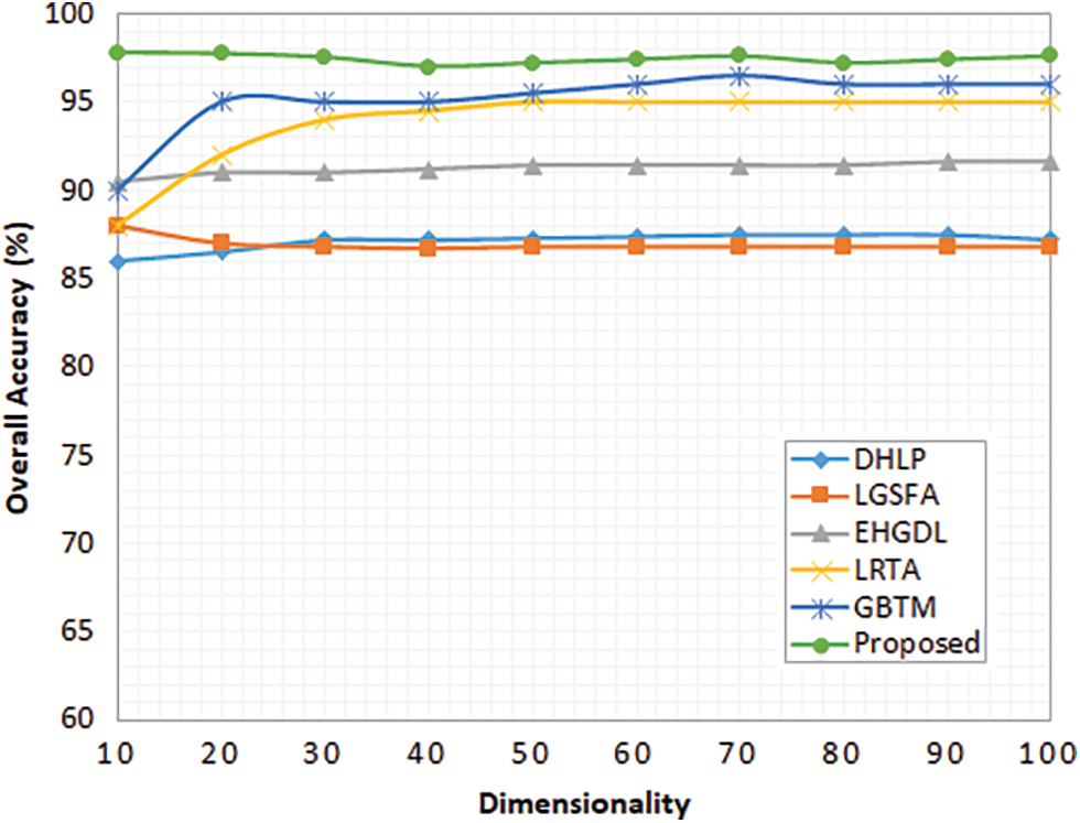
Figure 3: Overall accuracy for different dimensionalities (University of Pavia dataset)

To validate the classifier performance, the proposed dimensionality reduction method and existing methods are comparatively analyzed and the performances are presented in Table 7.

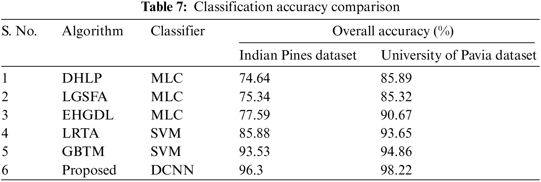
The existing methods like DHLP, LGSFA, and EHGDL incorporate a maximum likelihood classifier, and the LRTA and GBTM methods incorporate an SVM as a classifier. The proposed model includes depth wise CNN model for final classification. The initial dimensionality reduction is performed through optimized SOM. The major issue in handling hyperspectral images is its dimensionality and the presented approach effectively reduces the dimensions and selects the optimal feature which improves the classification accuracy compared to existing methods. The computation complexity of the proposed model is slightly higher than the existing methods due to multiple algorithms. However, it can be neglected as the results of the proposed dimensionality reduction method and classifier performances in hyperspectral image classification are observed as better compared to existing methods.

5  Conclusion

In this research work, the proposed depth-wise CNN model is used as a pre-processing technique to remove the general noises in the used datasets. The pre-processed image is then fed into the optimized SOM for solving the dimensionality reduction problem. The weight in the SOM is optimized by using WSOA, which is briefly explained in Section 3. The experiments are conducted on IP and UP datasets. The suggested model obtained 98% of AA and Kappa, whereas the previous models achieved 91% to 95% of AA and Kappa on the IP dataset. However, because of the huge number of parameters and the little quantity of training data required to train the model, deep neural network models such as CNN are prone to overfitting. Overfitting difficulties will be addressed in future studies by employing effective deep-learning approaches considering spatial resolution and spectral bandwidth.

Funding Statement: The authors received no specific funding for this study.

Conflicts of Interest: The authors declare that they have no conflicts of interest to report regarding the present study.

References

1. N. Liu, P. A. Townsend and Y. Wang, “Hyperspectral imagery to monitor crop nutrient status within and across growing seasons,” Remote Sensing Environment, vol. 255, no. 1, pp. 112–303, 2021. [Google Scholar]

2. X. Lyu, X. Li, D. Dang, M. Li and J. Gong, “A new method for grassland degradation monitoring by vegetation species composition using hyperspectral remote sensing,” Ecological Indicators, vol. 114, no. 2, pp. 106–310, 2020. [Google Scholar]

3. A. Guo, W. Huang and Y. Dong, “Wheat yellow rust detection using UAV-based hyperspectral technology,” Remote Sensing Environment, vol. 13, no. 2, pp. 123–128, 2021. [Google Scholar]

4. P. Huang, Q. Guo, C. Hanand and C. Zhang, “An improved method combining ANN and 1D-var for the retrieval of atmospheric temperature profiles from FY-4A/GIIRS hyperspectral data,” Remote Sensing Environment, vol. 13, no. 2, pp. 481–490, 2021. [Google Scholar]

5. M. A. Calin, A. C. Calin and D. N. Nicolae, “Application of airborne and spaceborne hyperspectral imaging techniques for atmospheric research: Past, present, and future,” Applied Spectroscopy Reviews, vol. 56, no. 2, pp. 289–323, 2021. [Google Scholar]

6. M. E. Paoletti, J. M. Haut, N. S. Pereira, J. Plaza and A. Plaza, “Ghostnet for hyperspectral image classification,” IEEE Transactions on Geoscience Remote Sensing, vol. 59, no. 2, pp. 10378–10393, 2021. [Google Scholar]

7. M. E. Paoletti, J. M. Haut, X. Tao, J. P. Miguel and A. Plaza, “A new GPU implementation of support vector machines for fast hyperspectral image classification,” Remote Sensing, vol. 12, no. 3, pp. 12–57, 2020. [Google Scholar]

8. D. Marinelli, F. Bovolo and L. Bruzzone, “A novel change detection method for multitemporal hyperspectral images based on binary hyperspectral change vectors,” IEEE Transactions on Geoscience Remote Sensing, vol. 57, no. 5, pp. 4913–4928, 2019. [Google Scholar]

9. Z. Hou, W. Li, L. Li, R. Tao and Q. Du, “Hyperspectral change detection based on multiple morphological profiles,” IEEE Transactions on Geoscience Remote Sensing, vol. 60, no. 3, pp. 550–572, 2021. [Google Scholar]

10. P. Ghamisi, N. Yokoya, J. Li and W. Liao, “Advances in hyperspectral image and signal processing: A comprehensive overview of the state of the art,” IEEE Transactions on Geoscience Remote Sensing, vol. 5, no. 4, pp. 37–78, 2017. [Google Scholar]

11. F. Feng, W. Li, Q. Du and B. Zhang, “Dimensionality reduction of hyperspectral image with graph-based discriminant analysis considering spectral similarity,” Remote Sensing Environment, vol. 9, no. 4, pp. 323–336, 2017. [Google Scholar]

12. N. Falco, J. A. Benediktsson and L. Bruzzone, “A study on the effectiveness of different independent component analysis algorithms for hyperspectral image classification,” IEEE Journals of Selected Topicsin Applied Earth Observation and Remote Sensing, vol. 7, no. 4, pp. 2183–2199, 2014. [Google Scholar]

13. C. Gordon, “A generalization of the maximum noise fraction transform,” IEEE Transactions on Geoscience and Remote Sensing, vol. 38, no. 2, pp. 608–610, 2000. [Google Scholar]

14. M. Sugiyama, “Dimensionality reduction of multimodal labeled data by local fisher discriminant analysis,” Journal of Machine Learning Research, vol. 8, no. 5, pp. 1027–1061, 2007. [Google Scholar]

15. Y. Zhou, J. Peng and C. Chen, “Dimension reduction using spatial and spectral regularized local discriminant embedding for hyperspectral image classification,” IEEE Transactions on Geoscience and Remote Sensing, vol. 53, no. 3, pp. 1082–1095, 2015. [Google Scholar]

16. X. Cao, T. Xiong and L. Jiao, “Supervised band selection using local spatial information for hyperspectral image,” IEEE Transactions on Geoscience and Remote Sensing Letter, vol. 13, no. 3, pp. 329–333, 2016. [Google Scholar]

17. Y. Dong, B. Du and L. Zhang, “Dimensionality reduction and classification of hyperspectral images using ensemble discriminative local metric learning,” IEEE Transactions on Geoscience and Remote Sensing, vol. 55, no. 5, pp. 2509–2524, 2017. [Google Scholar]

18. Z. Xue, S. Yang and M. Zhang, “Shape-adaptive tensor factorization model for dimensionality reduction of hyperspectral images,” IEEE Access, vol. 7, no. 2, pp. 115160–115170, 2019. [Google Scholar]

19. R. Mohanty, S. L. Happy and A. Routray, “Spatial–Spectral regularized local scaling cut for dimensionality reduction in hyperspectral image classification,” IEEE Transactions on Geoscience and Remote Sensing Letters, vol. 16, no. 6, pp. 932–936, 2019. [Google Scholar]

20. L. Yang, R. Zhang, S. Yang and L. Jiao, “Hyperspectral image classification via slice sparse coding tensor based classifier with compressive dimensionality reduction,” IEEE Access, vol. 8, no. 2, pp. 145207–145215, 2020. [Google Scholar]

21. G. Shi, H. Huang and L. Wang, “Unsupervised dimensionality reduction for hyperspectral imagery via local geometric structure feature learning,” IEEE Transactions on Geoscience and Remote Sensing Letters, vol. 17, no. 8, pp. 1425–1429, 2020. [Google Scholar]

22. Y. Deng, H. Li, X. Song, Y. Sun, X. Zhang et al., “Patch tensor-based multigraph embedding framework for dimensionality reduction of hyperspectral images,” IEEE Transactions on Geoscience and Remote Sensing, vol. 58, no. 3, pp. 1630–1643, 2020. [Google Scholar]

23. Y. Duan, H. Huang, Y. Tang, Y. Li and C. Pu, “Semisupervised manifold joint hypergraphs for dimensionality reduction of hyperspectral image,” IEEE Transactions on Geoscience and Remote Sensing Letters, vol. 18, no. 10, pp. 1811–1815, 2021. [Google Scholar]

24. T. Zhang, C. Shi, D. Liao and L. Wang, “A spectral spatial attention fusion with deformable convolutional residual network for hyperspectral image classification,” Remote Sensing, vol. 13, no. 2, pp. 76–90, 2021. [Google Scholar]

25. S. Sabour, N. Frosst and G. E. Hinton, “Dynamic routing between capsules,” arXiv:1710.09829, 2017. [Google Scholar]

26. R. Lei, C. Zhang, W. Liu, L. Zhang, X. Zhang et al., “Hyperspectral remote sensing image classification using deep convolutional capsule network,” IEEE Journals on Selected Topicsin Applied Earth Observations and Remote Sensing, vol. 14, no. 2, pp. 8297–8315, 2021. [Google Scholar]

27. J. Wang, S. Guo, R. Huang, L. Li, X. Zhang et al., “Dual-channel capsule generation adversarial network for hyperspectral image classification,” IEEE Transactions on Geoscience and Remote Sensing, vol. 60, no. 2, pp. 1–16, 2022. [Google Scholar]

28. D. Hong, L. Gao, N. Yokoya, J. Yao, J. Chanussot et al., “More diverse means better: Multimodal deep learning meets remote-sensing imagery classification,” IEEE Transactions on Geoscience and Remote Sensing, vol. 59, pp. 1–15, 2020. [Google Scholar]

29. X. Wu, D. Hong and J. Chanussot, “Convolutional neural networks for multimodal remote sensing data classification,” IEEE Transactions on Geoscience and Remote Sensing, vol. 60, pp. 1–10, 2022. [Google Scholar]

30. D. Hong, L. Gao, J. Yao, B. Zhang, A. Plaza et al., “Graph convolutional networks for hyperspectral image classification,” IEEE Transactions on Geoscience and Remote Sensing, vol. 59, no. 7, pp. 5966–5978, 2021. [Google Scholar]

31. A. Sellami, M. Farah, I. R. Farah and B. Solaiman, “Hyperspectral imagery classification based on semi-supervised 3-D deep neural network and adaptive band selection,” Expert Systems with Applications, vol. 129, no. 4, pp. 246–259, 2019. [Google Scholar]

32. T. Zhang, C. Shi, D. Liao and L. Wang, “A spectral spatial attention fusion with deformable convolutional residual network for hyperspectral image classification,” Remote Sensing, vol. 13, no. 2, pp. 35–90, 2021. [Google Scholar]

33. T. Zhang, C. Shi, D. Liao and L. Wang, “Deep spectral spatial inverted residual network for hyperspectral image classification,” Remote Sensing, vol. 13, no. 4, pp. 44–72, 2021. [Google Scholar]

34. Y. S. Luo, X. L. Zhao, T. X. Jiang, Y. B. Zheng and Y. Chang, “Hyperspectral mixed noise removal via spatial–spectral constrained unsupervised deep image prior,” IEEE Journal of Selected Topics in Applied Earth Observations and Remote Sensing, vol. 14, no. 4, pp. 9435–9449, 2021. [Google Scholar]

35. Z. Y. Zeng, T. Z. Huang, Y. Chen and X. L. Zhao, “Nonlocal block-term decomposition for hyperspectral image mixed noise removal,” IEEE Journal of Selected Topics in Applied Earth Observations and Remote Sensing, vol. 14, no. 2, pp. 5406–5420, 2021. [Google Scholar]

36. C. Wang, M. Xu, Y. Jiang, G. Zhang, H. Cui et al., “Translution-SNet: A semisupervised hyperspectral image stripe noise removal based on transformer and CNN,” IEEE Transactions on Geoscience and Remote Sensing, vol. 60, no. 2, pp. 1–14, 2022. [Google Scholar]

37. K. A. AlAfandy, H. Omara, M. Lazaar and M. Al Achhab, “Deep learning,” in Approaches and Applications of Deep Learning in Virtual Medical Care, 1st ed., USA: IGI Global, Chapter 6, pp. 127–167, 2022. [Google Scholar]

38. A. Kaveh, M. I. Ghazaanand and A. Asadi, “An improved water strider algorithm for optimal design of skeletal structures,” Periodica Polytechnica: Civil Engineering, vol. 64, no. 4, pp. 1284–1305, 2020. [Google Scholar]

39. A. Kaveh and A. DadrasEslamlou, “Water strider algorithm: A new metaheuristic and applications,” Structures, vol. 25, pp. 520–541, 2020. [Google Scholar]

40. F. Luo, T. Guo, Z. Lin, J. Ren and X. Zhou, “Semi supervised hypergraph discriminant learning for dimensionality reduction of hyperspectral image,” IEEE Journal of Selected Topics in Applied Earth Observations and Remote Sensing, vol. 13, no. 3, pp. 4242–4256, 2020. [Google Scholar]

41. J. An, X. Zhang and L. C. Jiao, “Dimensionality reduction based on group-based tensor model for hyperspectral image classification,” IEEE Transactions on Geoscience and Remote Sensing Letters, vol. 13, no. 10, pp. 1497–1501, 2016. [Google Scholar]