Deep Learning Based Vehicle Detection and Counting System for Intelligent Transportation

1  Introduction

Recently, real-time traffic monitoring has gained widespread interest with intelligent transportation systems (ITS) advancement. To constitute a reliable and robust ITS, vehicle counting and detection were considered to be the most imperative parts of analyzing and collecting large-mode traffic data [1]. Specifically, it serves a significant role in several real-world circumstances, like resolving traffic congestion issues and enhancing traffic safety. There were several remote sensing (RS) platforms available, which include terrestrial platforms (i.e., terrestrial laser scanning, farming robots, stationary photography, mobile mapping data), airplanes, satellites, and drones that can be leveraged for gaining data in various environmental monitoring researchers [2]. Among them, satellite remote sensing (RS) technology is scaled up to support worldwide environmental monitoring regularly. To support these efforts, several satellites specialized in collecting Earth observation data were launched recently [3]. Most support open access to the dataset for further stimulating the advancement of RS tools related to data from such missions. Such satellite missions commonly obtain optical images (in the normal channels of blue, red, and green). However, a key feature was multispectral images collected by instruments, including bands tuned, enhancing performance compared to optical sensors in numerous atmospheres and ecology sensing applications [4].

The study of intellectual earth observation to analyze and understand such aerial and satellite images has received widespread attention [5–8]. The main goal of the object counting task was to predict the object count of some class in a specified image, which serves a vital role in video and image analysis for the applications like urban planning, crowd behavior analysis, traffic monitoring, public security, and so on [6]. It is important to count vehicles in the traffic, which is expected to alleviate traffic congestion and raise traffic light efficiency. Online vehicle count through movements of interest (MOI) was to identify the total number of vehicles that are respective to MOI in an online paradigm [9–11]. Yet, precise vehicle counting becomes a challenge at crowded intersections because of the problems like the occlusions among poor weather conditions and particular vehicles. Also, the arrival period when vehicles move out of the region of interest (ROI) is computed [12].

The advancement of deep learning (DL) and object counting attained great performance in natural images, and some works have enforced object counting in RS images [13]. But because of the gap between natural and RS images, there will be great space for enhancement in RS object counting. The prevailing object counting technique is of two types: regression-based and detection-based. Detection-based techniques gain the number of objects by counting the identified bounding boxes. Counting vehicles related to traffic videos displays great benefits when a comparison is made to conventional vehicle-counting technology [10]. The video-related technique depends upon complicated image-processing methods over software. A traffic surveillance camera will be more convenient to install and maintain and cost less than conventional detectors [14,15]. More significantly, the information gained with traffic videos was viewed in real-time and more flexibly and efficiently.

This article presents a deep learning-based vehicle detection and counting system for ITS (DLVDCS-ITS) in remote sensing images. The presented DLVDCS-ITS technique intends to detect vehicles, count vehicles, and classify them into different classes. At the initial stage, the DLVDCS-ITS technique applies an improved RefineDet method for vehicle detection. Next, the Gaussian Mixture Model (GMM) is employed for the vehicle counting process. Finally, sooty tern optimization (STO) with a deep convolutional autoencoder (DCAE) model is used for vehicle classification. A brief experimental analysis is made to show the enhanced performance of the DLVDCS-ITS approach.

2  Related Works

Guo et al. [16] presented a density map-based vehicle counting methodology for remote sensing image (RSI) with constrained resolution. The density map-oriented model regards vehicle counting tasks as approximating the density of vehicle targets to the pixel value. The author proposes an enhanced convolutional neural network (CNN)-based system, named Congested Scene Recognition Network Minus (CSRNet—), which produces density maps of vehicles from input RSI. Yin et al. [17] developed a novel methodology for counting vehicles in a human-like manner. The study comprises two major contributions. Initially, the author proposes an effective light weighted vehicle count technique. The approach count is based on vehicle identity comparison to neglect duplicate examples. Integrated with spatiotemporal data between frames, it can improve accuracy and accelerate the speed of counting. Next, the author reinforces the model's performance by presenting an enhanced loss function based on Siamese neural network.

Zhao et al. [18] introduced vehicle counting through intra-resolution time continuity and cross-resolution spatial consistency constraints. First, a segmentation map is attained using semantic segmentation with previous data. The vehicle coverage rate regarding located parking lot was estimated and later transformed into vehicle region. Lastly, the relationships between the vehicles and the area can be determined using regression. Reference [19] proposed a vehicle counting framework for eliminating the problem of redundant vehicle data count while a vehicle has performed in consecutive frames of drone video. This study presents a comparison of concatenated 3 feature vectors for recognizing similar vehicles in the aerial video. Azimi et al. [20] developed joint vehicle segmentation and counting methodology relevant to the atrous convolutional layer. This technique employs a multi-task loss function for instantaneously reducing vehicle counting errors and pixel-wise segmentation. Furthermore, the rectangular shape of vehicle segmentation is refined through morphological operation.

Zheng et al. [21] developed a packaged solution that integrates a novel target tracking and moving vehicle counting methodology and an enhanced long short term memory (LSTM) network for forecasting traffic flow with meteorological. Especially, the MultiNetV3 framework and dynamic convolution network (DCN) V2 convolution kernel were utilized for replacing the You only look once (YOLO)v4 convolution kernel and backbone networks for realizing multiple target counting and tracking correspondingly. Consequently, integrated with temporal features of past traffic flow, the study presents weather condition in LSTM and realize short-term prediction of traffic flow at road junction levels. Asha et al. [22] developed a video-related vehicle counting methodology in a highway traffic video captured through a handheld camera. The video processing can be accomplished in three stages: counting, object detection using YOLO (You Only Look Once) and tracking with a correlation filter. YOLO achieved outstanding results in the object detection area, and the correlation filter accomplished competitive speed and great accuracy in tracking. Therefore, the author builds multiple object tracking with correlation filters through the bounding box produced using the YOLO architecture.

3  The Proposed Model

In this article, a new DLVDCS-ITS algorithm was devised for vehicle detection and counting system using remote sensing images. The presented DLVDCS-ITS technique intends to detect vehicles, count vehicles, and classify them into different classes. At the initial level, the DLVDCS-ITS approach applies an improved RefineDet method for vehicle detection. Next, GMM is employed for the vehicle counting process. At last, the STO algorithm with the DCAE model is used for vehicle classification. Fig. 1 defines the workflow of the DLVDCS-ITS mechanism.

Figure 1: Workflow of DLVDCS-ITS system

3.1 Vehicle Detection Module

Firstly, the vehicles are detected by the use of an improved RefineDet model. In the first phase, this improved RefineDet framework is employed for the vehicle detection present. The presented method makes use of VGG16 architecture as a backbone network, creates the sequence of anchors having distinct feature ratios and different scales from all feature-mapped cells by employing anchor-generated procedure of region proposal network [23], and accomplishes a predetermined quantity of vehicle bounding boxes following by 2 regression and classification, along with the probability of the incidence of different classes under this bounding box. Finally, the outcomes of regression and classification are accomplished with non-maximum suppression (NMS). The presented model was divided into a transfer connection block (TCB), anchor refinement module (ARM), and vehicle detection module (ODM). Fig. 2 demonstrates the structure of the RefineDet system.

Figure 2: Architecture of RefineDet

3.1.1 ARM Module

The ARM has been mainly gathered from a more convolutional layer and core network. The ARM mainly performs negative anchor (NA) filtering, refinement, generation, and feature extraction [24]. The anchor refinement is to change the size and place of anchor boxes, and the NA filter indicates the ARM when the confidence of the negative instance is higher than 0.99; this approach eliminates it and does not exploit it to final recognition from ODM. The NA filter filtered NA boxes with well-classification, further mitigating imbalance instances. In the feature extraction, 2 convolution layers, for example, ConVo6_1 and ConVo6_2, were further at the last of the VGG16 network. Then, add 4 new convolution layers, ConVo8_2, ConVo7_1, ConVo7_2, and ConVo8_1, for capturing higher-level (HL) semantic information from these techniques. Later, the combined features are transferred to the lower-level (LL) feature via TCB; however, the LL feature maps are employed for detecting that has maximal semantic information and improve the recognition performance of floating vehicles.

3.1.2 TCB Module

The TCB is commonly employed for linking ODM and ARM and transmitting the feature dataset of ARM to ODM. In addition, based on the FPN infrastructure, adjacent TCB is interconnected to realize the feature fusion of LL and HL characteristics and improve semantic information of LL features.

3.1.3 ODM Module

The ODM is the output set of TCB and prediction layer (regression and classification layers, viz., Conv. layers with the size of the kernel 3 × 3). Also, the resulting prediction layer was a specific kind of refined anchor and coordinate offset relative to refined anchor boxes. The refined anchor has been employed as input to further regression and classification, and final bounding boxes have been selected according to non-maximal suppression (NMS).

3.2 Vehicle Counting Module

At this stage, the detected vehicles are counted by the GMM model. For vehicle counting, a GMM can be utilized for background deduction in a complicated atmosphere for recognizing the areas of moving objects [25]. The GMM was dependable in foreground segmentation and background extraction procedure. Thus the features of moving items in video surveillance will be easy to identify. It was a density model comprising Gaussian function elements. This technique is leveraged for executing the background extraction procedure because it is very reliable towards repetitive object detection scenarios and light variances.

The Gaussian mixture model for computing the variance and mean is expressed as:

P(xi)=∑i=1Kwi,t×1(2π)(n2)|ϕi,l|e12(xt−μi,t)TΣi,t−1(xt−μi,t).(1)

where, μ(i,t)= mean value of Gaussian distribution at time t,

ϕ(i,t)=covariance matrix,

K = number of distributions.

3.3 Vehicle Classification Module

At the final stage, the STO algorithm with the DCAE model is used for vehicle classification. Autoencoder (AE) is a standard deep neural network (DNN) infrastructure which generates utilization of their input as a label. Afterwards, the network tries to recreate its input in the learning process [26]; in this regard, it creates and automatically removes the representation features from the appropriate time iterations. This type of network was generated by stacking deep layers from AE methods containing 2 important parts of decoding and encoding. DCAE was a type of AE executed convolutional layer for determining the inner data of images. During the DCAE, infrastructure weighted has shared betwixt all the locations in each feature map, decreasing parameter redundancy and maintaining spatial locality. To extract the deep features, assume that H, D, and W denote the corresponding height, depth, and width of datasets, and n indicates the pixel counts. To all the members of the X set, image patches with 7×7×D size are extracted, whereas χj stands for central pixels. Therefore, the X set was considered an image patch; all the patches, xi∗, are provided as encoded blocks. To input xi∗, a hidden layer map of the kth feature map can be demonstrated under the:

hk=σ(xi∗∗Wk+bk)(2)

In Eq. (2), b denotes the bias; σ refers to the activation function, and the symbol ∗ equals the 2-D convolutional layer, and it can be obtained by subsequent demonstrated as:

y=σ(∑k∈Hhk∗W~k+b~k)(3)

In Eq. (3), bias b occurs to all the input channels, and h represents a group of latent feature maps. The W~ equivalent to the flip function over both dimensional weights W. y stands for predictive value. For determining the parameter vector representing the whole DCAE infrastructure, one could minimalize the succeeding cost function represented as:

E(θ)=1n∑i=1n‖xi∗−yi‖22(4)

To minimize this function, it can be required for evaluating the gradient of cost functions regarding the convolution kernel (W,W~) and bias (b,b~) parameter:

∂E(θ)∂Wk=x∗∗δhk+hk∗δy(5)

∂E(θ)∂bk=δhk+δy(6)

At this point, δh and δy correspond for deltas of the hidden layer and reconstruction. Afterwards, the weight was upgraded by the optimized technique. Finally, the DCAE parameter has been estimated if loss function convergence has been executed. The resultant feature mapping of the encoded block was assumed as a deep feature. During this case, batch normalization (BN) has been utilized to tackle the internal covariant shift phenomenon and improve the performance of networks using normalized input layers with re-scaling and re-centring. The BN supports increasing accuracy and more to learn.

The STO algorithm adjusts the DCAE parameters. The STO technique was desired over other optimized techniques because of the following details: The STO technique was able for local optima avoidance, exploration, and exploitation [27,28]. It can resolve difficult, constrained issues and is highly competitive and related to other optimized approaches. The STO approach has been simulated by the attack efficiency of the sooty tern (ST) bird. Generally, the STs live in groups. It employs its intelligence to place and attacks the targets. The most prominent features of STs were assault and migration performances. The succeeding offered insights as to ST birds:

•   The ST was simulated in the group from migration. To avoid a collision, the initial locations of STs are dissimilar.

•   In the groups, the ST with the least fitness level yet travelled the same distance that the fittest betwixt them could.

•   Based on the fittest STs, the lowest fitness STs were upgraded in primary locations.

The ST is essential for meeting 3 necessities in the migration: SA has been employed to calculate a novel searching agent position to ignore collisions with neighbourhood searching agents (i.e., STs).

C→st=sA⋅P→(z)(7)

where C→st represents the location of STs that could not collide with other terns, P→st defines the present location of STs. z implies the present iteration, and sA represents the migration of STs in the solution spaces. Afterwards, the collision evasion search agent converged in the path of the finest neighbor.

M→st=CB⋅P→st(z)(P→bst(z)−P→st(z))(8)

M→St denotes the particular location of search agents (i.e., ST). P→bst(z) defines the optimal location to search agents, and CB implies the arbitrary variable and is computed as:

CB=0.5Rand(9)

Whereas Rand refers to any arbitrary number between 0 and 1. Upgrade equal to optimal searching agents: At last, the STs have reviewed its location regarding the optimal search agents.

D→st=C→st+M→st(10)

whereas D→st refers to variance betwixt the search agents and optimal fittest search agents. The ST has been changing its attack and speed angles in migration. It attained altitude by flapping its wing. It can create spherical acts in the air and then attack prey, as explained below:

x′=Radiussin⁡(i)(11)

y′=Radiuscos⁡(i)(12)

z′=Radiusi(13)

r=uekv(14)

whereas Radius implies the spiral radius, i lies in [0≤k≤2τc], and u and v determine the constant value.

4  Performance Evaluation

This section examines the vehicle detection, counting, and classification outcomes of the DLVDCS-ITS model on a dataset including 3000 images. The dataset holds 1000 images under three class labels: car, bus, and truck, as represented in Table 1.

The confusion matrices generated during the vehicle classification process are shown in Fig. 3. The figures indicated that the DLVDCS-ITS model has correctly recognized all the car, bus, and truck images proficiently.

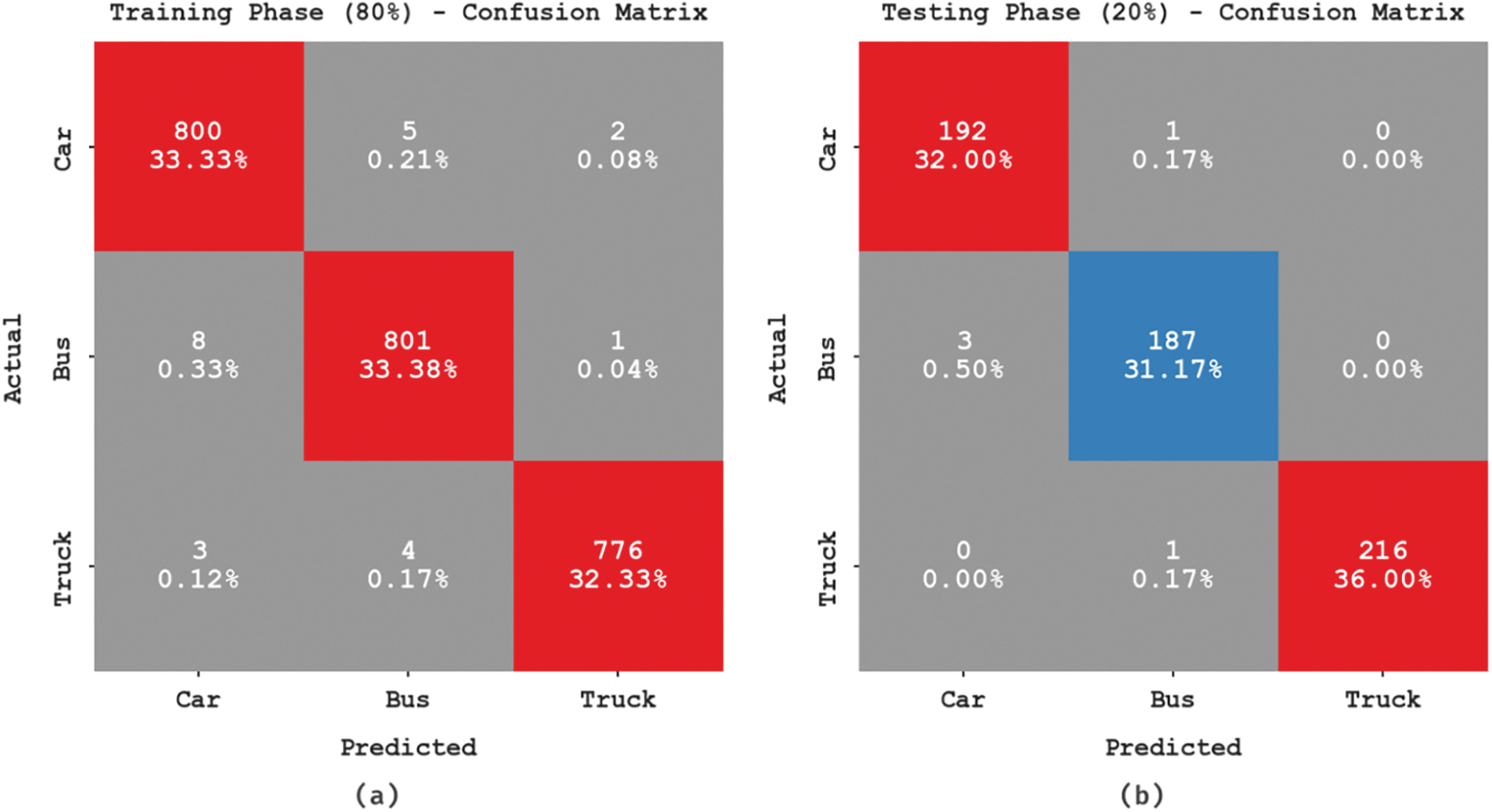
Figure 3: Confusion matrices of DLVDCS-ITS system (a–b) TR and TS dataset of 80:20 and (c–d) TR and TS dataset of 70:30

Table 2 reports the entire vehicle classifier output of the DLVDCS-ITS technique on 80:20 of the training (TR)/testing (TS) dataset. Fig. 4 displays the vehicle classifier outcomes of the DLVDCS-ITS method on 80% of the TR dataset. The experimental values indicated that the DLVDCS-ITS model has proficiently identified all the vehicles on 80% of the TR dataset. It is noted that the DLVDCS-ITS model has attained an average accuy of 99.36%, precn of 99.05%, recal of 99.04%, Fscore of 99.05%, and Gmean of 99.28%.

Figure 4: Vehicle classification outcome of DLVDCS-ITS system in 80% of the TR dataset

Fig. 5 exhibits the vehicle classifier outcomes of the DLVDCS-ITS methodology on 20% of the TS dataset. The simulation values exhibited that the DLVDCS-ITS approach proficiently recognized all the vehicles on 20% of the TS dataset. It is noticed that the DLVDCS-ITS method has achieved an average accuy of 99.44%, precn of 99.13%, recal of 99.15%, Fscore of 99.14%, and Gmean of 99.37%.

Figure 5: Vehicle classification outcome of DLVDCS-ITS system in 20% of the TS dataset

Table 3 reports the entire vehicle classifier outcomes of the DLVDCS-ITS methodology on 70:30 of the TR/TS dataset. Fig. 6 exemplifies the vehicle classifier result of the DLVDCS-ITS method on 70% of the TR dataset. The outcome denoted by the DLVDCS-ITS algorithm has proficiently identified all the vehicles on 70% of the TR dataset. It is pointed out that the DLVDCS-ITS approach has reached an average accuy of 99.24%, precn of 98.86%, recal of 98.86%, Fscore of 98.86%, and Gmean of 99.14%.

Figure 6: Vehicle classification outcome of DLVDCS-ITS system in 70% of the TR dataset

Fig. 7 portrays the vehicle classifier outcomes of the DLVDCS-ITS algorithm on 30% of the TS dataset. The simulation values show the DLVDCS-ITS methodology has proficiently detected all the vehicles on 30% of the TS dataset. It is highlighted that the DLVDCS-ITS methodology has achieved an average accuy of 98.52%, precn of 97.79%, recal of 97.79%, Fscore of 97.78%, and Gmean of 98.34%.

Figure 7: Vehicle classifier outcome of DLVDCS-ITS system in 30% of the TS dataset

The TR accuracy (TRA) and validation accuracy (VLA) gained by the DLVDCS-ITS method under the test dataset is exhibited in Fig. 8. The outcome exhibited by the DLVDCS-ITS approach has attained supreme TRA and VLA values. Predominantly the VLA is bigger than TRA.

Figure 8: TRA and VLA analysis of DLVDCS-ITS system

The TR loss (TRL) and validation loss (VLL) of the DLVDCS-ITS algorithm on the TS dataset are shown in Fig. 9. The result exhibited the DLVDCS-ITS technique has recognized the least TRL as well as VLL.

Figure 9: TRL and VLL analysis of DLVDCS-ITS system

A clear precn−recal investigation of the DLVDCS-ITS approach on the TS data is shown in Fig. 10. The results designated the DLVDCS-ITS algorithm have improved theprecn−recal outcomes under all classes.

Figure 10: Precision-recall analysis of the DLVDCS-ITS system

Table 4 portrays a brief accuy examination of the DLVDCS-ITS model with other existing methods [29,30]. The results inferred that the speeded up robust features (SURF) model reached the least accuy of 45.82%, whereas the scale-invariant feature transform (SIFT) and histogram of gradients (HOG) models have reached closer accuy of 62.78% and 69.46%, respectively. Although the AlexNet, VGGNet, and ResNet models have resulted in reasonable accuy of 89.37%, 94.35%, and 96.04%, the DLVDCS-ITS model outperforms the other ones with higher accuy of 99.44%.

Finally, detailed results of the DLVDCS-ITS model and existing methods are given in Table 5. The results implied the Faster region based convolutional neural network (RCNN) method had shown poor performance. At the same time, the YOLO, single shot detector (SSD), and enhanced-SSD models have obtained closer vehicle counting performance.

But the DLVDCS-ITS model has shown better performance with full correctness of 99.15%, completeness of 92.37%, and quality of 91.68%. Therefore, the DLVDCS-ITS model can be employed for accurate vehicle detection and counting.

5  Conclusion

This article formulated a new DLVDCS-ITS algorithm for vehicle detection and counting system using remote sensing images. The presented DLVDCS-ITS technique intends to detect vehicles, count vehicles, and classify them into different classes. At the initial level, the DLVDCS-ITS method applies an improved RefineDet algorithm for vehicle detection. Next, GMM is employed for the vehicle counting process. At last, the STO algorithm with the DCAE model is used for vehicle classification. A brief simulation analysis was done to demonstrate the enhanced performance of the DLVDCS-ITS technique. The comparison study demonstrates the supremacy of the presented DLVDCS-ITS technique over the recent state-of-the-art approaches. Thus, the presented DLVDCS-ITS approach can be exploited for real-time traffic monitoring. In future, we will extend to generate density maps of the vehicles and license plate number recognition.

Acknowledgement: Not applicable.

Funding Statement: This research was supported by the National Research Foundation of Korea (NRF) grant funded by the Korea government (MSIT) (No. 2021R1A4A1031509).

Author Contributions: Conceptualization: A. Vikram and J. Akshya. Data curation and Formal analysis: J. Akshya and L. Jerlin Rubini. Investigation and Methodology: Sultan Ahmad. Project administration and Resources: Supervision; Seifedine Kadry. Validation and Visualization: Oscar Castillo, Seifedine Kadry. Writing–original draft, A. Vikram. Writing–review and editing, A. Vikram and Jungeun Kim. All authors have read and agreed to the published version of the manuscript.

Availability of Data and Materials: Not applicable.

Conflicts of Interest: The authors declare that they have no conflicts of interest to report regarding the present study.

References

1. E. Kilic and S. Ozturk, “An accurate car counting in aerial images based on convolutional neural networks,” Journal of Ambient Intelligence and Humanized Computing, pp. 1–10, 2021. https://doi.org/10.1007/s12652-021-03377-5. [Google Scholar] [CrossRef]

2. A. Froidevaux, A. Julier, A. Lifschitz, M. T. Pham, R. Dambreville et al., “Vehicle detection and counting from VHR satellite images: Efforts and open issues,” in GARSS-2020 IEEE Int. Geoscience and Remote Sensing Symp., Waikoloa, HI, USA, pp. 256–259, 2020. [Google Scholar]

3. S. Karnick, M. R. Ghalib, A. Shankar, S. Khapre and I. A. Tayubi, “A novel method for vehicle detection in high-resolution aerial remote sensing images using YOLT approach,” Multimedia Tools and Applications, vol. 81, no. 17, pp. 23551–23566, 2022. [Google Scholar]

4. Q. Meng, H. Song, Y. A. Zhang, X. Zhang, G. Li et al., “Video-based vehicle counting for expressway: A novel approach based on vehicle detection and correlation-matched tracking using image data from PTZ cameras,” Mathematical Problems in Engineering, vol. 2020, no. 9, pp. 1–16, 2020. [Google Scholar]

5. Z. Dai, H. Song, X. Wang, Y. Fang, X. Yun et al., “Video-based vehicle counting framework,” IEEE Access, vol. 7, pp. 64460–64470, 2019. [Google Scholar]

6. A. Khan, K. S. Khattak, Z. H. Khan, M. A. Khan and N. Minallah, “Cyber physical system for vehicle counting and emission monitoring,” International Journal of Advanced Computer Research, vol. 10, no. 50, pp. 1–13, 2020. [Google Scholar]

7. S. Singh, B. Singh, B. Singh and A. Das, “Automatic vehicle counting for IoT based smart traffic management system for Indian urban settings,” in 4th Int. Conf. on Internet of Things: Smart Innovation and Usages (IoT-SIU), Ghaziabad, India, pp. 1–6, 2019. [Google Scholar]

8. A. A. Alsanabani, M. A. Ahmed and A. M. Al Smadi, “Vehicle counting using detecting-tracking combinations: A comparative analysis,” in 4th Int. Conf. on Video and Image Processing (ICVIP), Xi’an China, pp. 48–54, 2020. [Google Scholar]

9. H. Ji, Z. Gao, T. Mei and B. Ramesh, “Vehicle detection in remote sensing images leveraging on simultaneous super-resolution,” IEEE Geoscience and Remote Sensing Letters, vol. 17, no. 4, pp. 676–680, 2019. [Google Scholar]

10. H. Zhou, L. Wei, C. P. Lim and S. Nahavandi, “Robust vehicle detection in aerial images using bag-of-words and orientation aware scanning,” IEEE Transactions on Geoscience and Remote Sensing, vol. 56, no. 12, pp. 7074–7085, 2018. [Google Scholar]

11. S. A. Ahmadi, A. Ghorbanian and A. Mohammadzadeh, “Moving vehicle detection, tracking and traffic parameter estimation from a satellite video: A perspective on a smarter city,” International Journal of Remote Sensing, vol. 40, no. 22, pp. 8379–8394, 2019. [Google Scholar]

12. H. Song, H. Liang, H. Li, Z. Dai and X. Yun, “Vision-based vehicle detection and counting system using deep learning in highway scenes,” European Transport Research Review, vol. 11, no. 1, pp. 1–16, 2019. [Google Scholar]

13. H. Yao, R. Qin and X. Chen, “Unmanned aerial vehicle for remote sensing applications—A review,” Remote Sensing, vol. 11, no. 12, pp. 1443, 2019. [Google Scholar]

14. R. Bibi, Y. Saeed, A. Zeb, T. M. Ghazal, T. Rahman et al., “Edge AI-based automated detection and classification of road anomalies in VANET using deep learning,” Computational Intelligence and Neuroscience, vol. 2021, no. 5, pp. 1–16, 2021. [Google Scholar]

15. S. Razakarivony and F. Jurie, “Vehicle detection in aerial imagery: A small target detection benchmark,” Journal of Visual Communication and Image Representation, vol. 34, no. 10, pp. 187–203, 2016. [Google Scholar]

16. Y. Guo, C. Wu, B. Du and L. Zhang, “Density map-based vehicle counting in remote sensing images with limited resolution,” ISPRS Journal of Photogrammetry and Remote Sensing, vol. 189, no. 4, pp. 201–217, 2022. [Google Scholar]

17. K. Yin, L. Wang and J. Zhang, “ST-CSNN: A novel method for vehicle counting,” Machine Vision and Applications, vol. 32, no. 5, pp. 1–13, 2021. [Google Scholar]

18. Q. Zhao, J. Xiao, Z. Wang, X. Ma, M. Wang et al., “Vehicle counting in very low-resolution aerial images via cross-resolution spatial consistency and intra-resolution time continuity,” IEEE Transactions on Geoscience and Remote Sensing, vol. 60, no. 4706813, pp. 1–13, 2022. [Google Scholar]

19. A. Holla, U. Verma and R. M. Pai, “Efficient vehicle counting by eliminating identical vehicles in UAV aerial videos,” in IEEE Int. Conf. on Distributed Computing, VLSI, Electrical Circuits and Robotics (DISCOVER), Udupi, India, pp. 246–251, 2020. [Google Scholar]

20. S. Azimi, E. Vig, F. Kurz and P. Reinartz, “Segment-and-count: Vehicle counting in aerial imagery using atrous convolutional neural networks,” International Archives of the Photogrammetry, Remote Sensing and Spatial Information Sciences-ISPRS Archives, vol. 42, pp. 1–5, 2018. [Google Scholar]

21. Y. Zheng, X. Li, L. Xu and N. Wen, “A deep learning-based approach for moving vehicle counting and short-term traffic prediction from video images,” Frontiers in Environmental Science, vol. 10, pp. 905443, 2022. [Google Scholar]

22. C. S. Asha and A. V. Narasimhadhan, “Vehicle counting for traffic management system using YOLO and correlation filter,” in IEEE Int. Conf. on Electronics, Computing and Communication Technologies (CONECCT), Bangalore, India, pp. 1–6, 2018. [Google Scholar]

23. H. Xie and Z. Wu, “A robust fabric defect detection method based on improved refinedet,” Sensors, vol. 20, no. 15, pp. 4260, 2020. [Google Scholar] [PubMed]

24. M. F. Alotaibi, M. Omri, S. A. Khalek, E. Khalil and R. F. Mansour, “Computational intelligence-based harmony search algorithm for real-time object detection and tracking in video surveillance systems,” Mathematics, vol. 10, no. 5, pp. 733, 2022. [Google Scholar]

25. K. Balaji, A. Chowhith and S. G. Desai, “Vehicle counting method based on Gaussian mixture models and blob analysis,” International Journal of Research Publication and Reviews, vol. 3, no. 6, pp. 2912–2917, 2022. [Google Scholar]

26. R. Marzouk, F. Alrowais, F. N. Al-Wesabi and A. M. Hilal, “Atom search optimization with deep learning enabled arabic sign language recognition for speaking and hearing disability persons,” Healthcare, vol. 10, no. 9, pp. 1–15, 2022. [Google Scholar]

27. M. A. Hamza, H. A. Mengash, S. S. Alotaibi, S. B. H. Hassine, A. Yafoz et al., “Optimal and efficient deep learning model for brain tumor magnetic resonance imaging classification and analysis,” Applied Sciences, vol. 12, no. 15, pp. 1–15, 2022. [Google Scholar]

28. J. He, Z. Peng, D. Cui, J. Qiu, Q. Li et al., “Enhanced sooty tern optimization algorithm using multiple search guidance strategies and multiple position update modes for solving optimization problems,” Applied Intelligence, vol. 267, no. 1, pp. 66, 2022. [Google Scholar]

29. J. Zhu, K. Sun, S. Jia, Q. Li, X. Hou et al., “Urban traffic density estimation based on ultrahigh-resolution UAV video and deep neural network,” IEEE Journal of Selected Topics in Applied Earth Observations and Remote Sensing, vol. 11, no. 12, pp. 4968–4981, 2018. [Google Scholar]

30. J. Gao, M. Gong and X. Li, “Global multi-scale information fusion for multi-class object counting in remote sensing images,” Remote Sensing, vol. 14, no. 16, pp. 1–15, 2022. [Google Scholar]