
 Submit a Paper
 Propose a Special lssue
 Open Access
ARTICLE

3D Reconstruction for Early Detection of Liver Cancer
1 Faculty of Computing and Artificial Intelligence, Benha University, Benha, 13511, Egypt
2 Faculty of Computers and Information Technology, The Egyptian E-Learning University, Giza, 12611, Egypt
* Corresponding Author: Rana Mohamed. Email:
Computer Systems Science and Engineering 2025, 49, 213-238. https://doi.org/10.32604/csse.2024.059491
Received 09 October 2024; Accepted 05 December 2024; Issue published 10 January 2025
 View Full Text
 Download PDF
Abstract
Globally, liver cancer ranks as the sixth most frequent malignancy cancer. The importance of early detection is undeniable, as liver cancer is the fifth most common disease in men and the ninth most common cancer in women. Recent advances in imaging, biomarker discovery, and genetic profiling have greatly enhanced the ability to diagnose liver cancer. Early identification is vital since liver cancer is often asymptomatic, making diagnosis difficult. Imaging techniques such as Magnetic Resonance Imaging (MRI), Computed Tomography (CT), and ultrasonography can be used to identify liver cancer once a sample of liver tissue is taken. In recent research, reliable detection of liver cancer with minimal computing computational complexity and time has remained a serious difficulty. This paper employs the DenseNet model to enhance the detection of liver nodules with tumors by segmenting them using UNet and VGG using Fastai (UVF) in CT images. Its dense interconnections distinguish the DenseNet between layers. These dense connections facilitate the propagation of gradients and the flow of information throughout the network, thereby enhancing the efficacy and performance of training. DenseNet’s architecture combines dense blocks, bottleneck layers, and transition layers, allowing it to achieve a compromise between expressiveness and computing efficiency. Finally, the 3D liver nodular models were created using a ray-casting volume rendering approach. Compared to other state-of-the-art deep neural networks, it is suitable for clinical applications to assist doctors in diagnosing liver cancer. The proposed approach was tested on a 3Dircadb dataset. According to experiments, UVF segmentation on the 3Dircadb dataset is 97.9% accurate. According to the study, the DenseNet and UVF segment liver cancer better than prior methods. The system proposes automated 3D liver cancer tumor visualization.Keywords
Glossary/Nomenclature/Abbreviations
| CT | Computed Tomography |
| MRI | Magnetic Resonance Imaging |
| EDCNN | Cascaded deep convolutional encoder-decoder neural networks |
| LVSNet | Liver Vessel Segmentation Network |
| UVF | UNet and VGG using Fastai |
| DenseNet | Densely Connected Convolutional Network |
| UNet | U-shaped convolutional neural network (CNN) architecture |
| VGG | Visual Geometry Group |
| RA-Net | Residual-Atrous U-Net |
| PrM | The Preprocessing Module |
| DM | The Detection Module |
| 3DRM | The three-dimensional Reconstruction Module |
| HU | Hounsfield units |
| CNN | Convolutional neural network |
| TL | Transfer learning |
| TP | True positives |
| FP | False positives |
| FN | False negatives |
| TN | True negatives |
| HIPAA | The Health Insurance Portability and Accountability Act |
| GDPR | The General Data Protection Regulation |
| ReLU | Rectified Linear Units |
| BN | Batch Normalization |
| Conv | Convolution |
| MSFF | Modified Single Fiber Filtration |
| 3D | Three-dimensional |
| DSC | Dice Similarity Coefficient |
| LITS | Liver Tumor Segmentation |
| DWAM | Dual-branch Attention Module |
| CAA | Channel-wise ASPP with Attention |
| MAPFUNet | Multi-scale Attention-guided and Progressive Feature Fusion Network |
| CRF | Conditional Random Field |
| MW-UNet | Multi-phase Weighted U-Net |
| kNN | k-Nearest Neighbors |
| PAB | Position-wise Attention Block |
| O-SHO | Opposition-based Spotted Hyena Optimization |
Liver cancer, a complex and often fatal disease, significantly impacts global health due to its high prevalence and aggressive nature. It is the sixth most common cancer worldwide, as depicted in Fig. 1a. Specifically, it is the fifth most prevalent cancer among men and the ninth among women, as shown in Fig. 1b,c [1]. Liver cancer arises when abnormal cells in the liver grow uncontrollably, forming a malignant tumor, which can be primary (originating within the liver) or secondary (spreading to the liver from other body areas). This condition presents substantial diagnostic and treatment challenges, compounded by risk factors such as chronic hepatitis B and C infections, excessive alcohol consumption, obesity, and non-alcoholic fatty liver disease [1]. Screening and incidental findings remain the primary diagnostic methods, yet many regions lack standardized screening programs, resulting in late-stage diagnoses in numerous cases [2]. Radiologists face additional challenges, such as distinguishing malignant from benign nodules in imaging, complicating the diagnostic process [3].
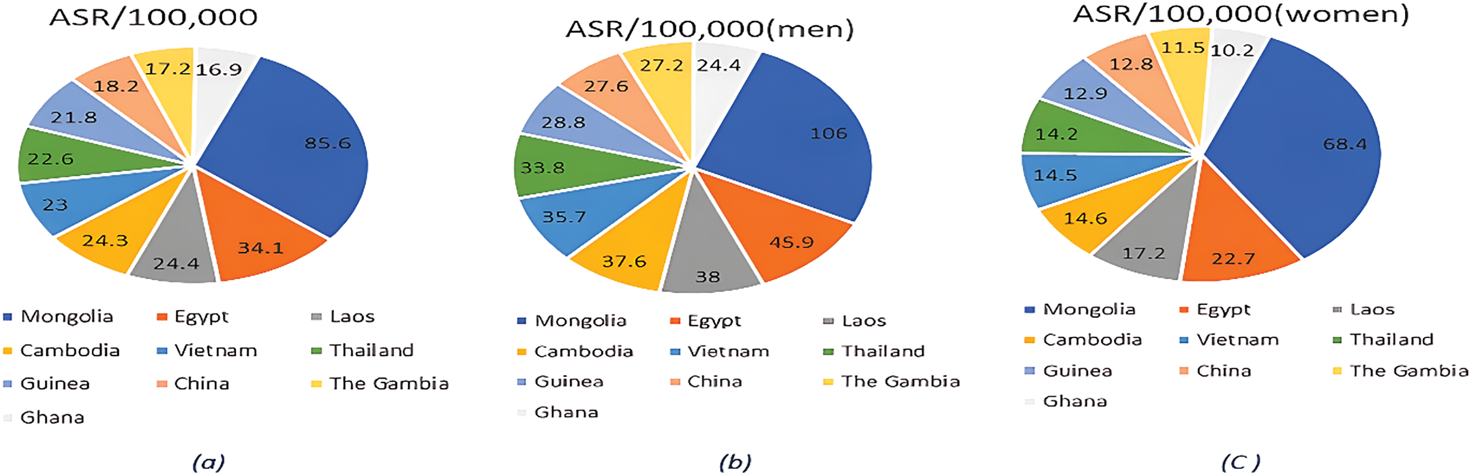
Figure 1: (a). Total global cancer incidence and rates in 2020: (b). The global incidence of cancer in men and its rates in 2020: (c). The global incidence of cancer in women and its rates in 2020
Furthermore, the combined efforts of researchers, healthcare professionals, and technological innovation are vital in the ongoing battle against liver cancer, facilitating the development of novel treatments and enhancing survival rates. Among these advancements, three-dimensional (3D) visualization techniques, including ray-casting that simulates light rays to produce detailed 3D views of complex liver structures and segmentation models such as UNet and VGG, implemented with Fastai that enable efficient and precise segmentation of liver lesions from medical imaging data, are critical for accurate diagnosis. These methods allow radiologists to accurately assess the spatial characteristics of liver lesions, aiding in personalized treatment planning. Various segmentation techniques, such as semi-automatic approaches utilizing Kullback-Leibler divergence and graph-cut methods [4], and manual and automated models like edge detectors [5], atlas-based models [6], deformable models [7], and graphical models [8], contribute to advancing diagnostic accuracy.
This research will review current literature and advancements in hepatic tumor segmentation to highlight key methodologies that contribute to improved management of liver cancer.
Despite these advancements, current models struggle with challenges such as distinguishing between benign and malignant nodules and handling complex tumor boundaries. Building upon the gaps identified in previous literature, the proposed system will analyze liver damage globally using deep learning methodologies, focusing on the entire CT image. This new approach for detecting tumors and identifying the liver in a CT image for liver cancer involves segmenting the liver, detecting tumors, and subsequently performing 3D reconstruction. Creating a 3D model enables lossless reconstruction, providing a more realistic image of the tumor compared to wired models based on tumor cell 3D reconstruction. This detailed 3D visualization will allow physicians to better understand the interaction between the tumor and its surrounding tissues, even before surgery, which is crucial for effective treatment planning.
The present study offers the following contributions:
(1) The system suggests a three-dimensional visualization technique for computer-aided liver nodule identification based on UVF, DenseNet, and the ray-casting volume rendering method.
(2) Classify liver nodules. The experimental results indicate that UVF is useful for segmenting and DenseNet classifying liver nodules.
The remainder of this paper is structured as follows: Section 2 reviews related work, providing context and background for this study. Section 3 explains the methodologies and materials, starting with the preprocessing steps for liver cancer detection and detailing the integration of UVF, DenseNet, and ray-casting techniques. Section 4 describes the datasets and provides a comprehensive experimental analysis, outlining the training, testing, implementation processes, evaluation metrics, and 3D reconstruction results. Section 5 offers an in-depth discussion of the outcomes, highlighting the comparison to existing methods and limitations of the proposed method. Finally, Section 6 concludes the study and proposes directions for future research.
Liver cancer research has advanced in diagnostics, with a growing emphasis on computational methods for biomarker analysis and imaging-based early detection. This section summarises key developments and ongoing challenges at the intersection of liver cancer research and computer science.
Budak et al. [9] used cascaded encoder-decoder architecture to get a dice score of 63.4%. Their approach is similar to that of segmenting tumors in two steps. The EDCNN architecture comprises two components: the initial component denotes the encoder. Next, we have the decoder network. The two components provide a symmetrical configuration. Multiple measures were employed to evaluate the suggested model. The utilization of the public dataset (3DIRCADb) is deemed difficult due to its substantial assortment and intricacy of livers and associated malignancies [10]. Utilizing twenty CT scans, of which seventy-five percent contain hepatic lesions, its performance is evaluated.
Furthermore, Tran et al. [11] developed a revised iteration of the U-Net model. by integrating layer-by-layer integration of dense connections. They got an awe-inspiring score of 73.34% compared to previous efforts. However, one of the significant concerns they mentioned in their suggested model is that as the number of convolution units increases, the model’s connection gets more complicated.
Yan et al. [12] introduced LVSNet, an innovative deep neural network designed to identify the precise structure of hepatic vessels for segmentation. In the present study, the utilization of publicly accessible liver datasets for deep learning purposes, such as 3Dircadb, Sliver072, and CHAOS challenge3, is seen. The empirical findings illustrate that the suggested LVSNet surpasses prior techniques on datasets for hepatic vascular segmentation. By achieving greater values for Sensitivity and Dice, the proposed method demonstrates the efficacy of the MSFF block. The UNet’s segmentation performance is enhanced by 2.9% in terms of Dice and segmentation accuracy, achieving a DSC of 90.4%.
Zhang et al. [13] introduced a 3D multi-attention guided multi-task learning network consisting of three cooperating components: the backbone, SA-shared feature learning, and feature learning. From three medical centers—Taiyuan People Hospital, China; Xian People Hospital, China; and Department of Radiology, China-Japan Friendship Hospital, Beijing, China—the dataset was obtained utilizing three medical instruments: Toshiba 320-slice CT, SOMATOM 64-slice CT, and Philips 128-slice CT. The dataset has been partitioned into two distinct subgroups: a training set of 131 scans and a test set consisting of 70 scans. The empirical findings indicate that our approach achieves an average Accuracy (Acc) value of 80.5%.
Other recent investigations on liver tumor segmentation involve the work of Han et al. [14]. Their approach applied a convolutional neural network based on boundary loss using a dice score of roughly 68% to segment the tumors. Similarly, Zhang et al. [15] proposed a Hybrid-3DResUNet to segregate tumors using 3D convolution techniques. Their suggested model performs quite well regarding dice soreness, scoring 78.58%.
Kalsoom et al. [16] developed a modified iteration of U- called Residual-Atrous U-Net (RA-Net) to segment liver tumors. The model is achieved by adopting U-Net as a foundational model and extracting the characteristics of the tumor through a parallel structure-based atomic convolution block integrated into the original U-Net. The proposed RA-Net gets an awe-inspiring score of 81%. The RA-Net employed involved the immediate segmentation of CT image-based cancers relative to the conventional two-stage technique commonly utilized in existing methodologies.
Manjunath et al. [17] developed a Unet58 layers architecture for liver and tumor segmentation. It represents the conventional deep convolution network, which results in the formation of a hepatic segmentation network. The improved Unet model performs better than existing deep-learning models in liver segmentation, with a high DSC score of 96.15%. Additionally, it outperforms existing models in tumor segmentation, achieving a DSC score of 89.38% for the LITS dataset of size 256 × 256. Additionally, using a 3Dircadb dataset with dimensions 128 × 128 and a segmentation score of 69.80% for tumors, a high DSC score of 91.94% was achieved.
Kumar et al. [18] proposed a hybrid multi-stage CNN model that integrates traditional image processing techniques with deep learning, achieving an accuracy of 87.5%. This approach emphasizes feature selection to reduce false positives but has limitations in generalizing to diverse and complex liver tumor cases, particularly when handling highly variable tumor characteristics. Patel et al. [19] utilized a multi-stage architecture combining edge detection with CNNs for liver tumor classification, achieving 86.7% accuracy. However, the model struggles with accurately segmenting tumors with irregular shapes or in cases of poor image quality, and the reliance on edge detection reduces robustness against imaging artifacts.
Lee et al. [20] developed a dual-path CNN model combining PET and CT data for tumor segmentation and survival risk prediction, achieving a Dice Similarity Coefficient of 0.7367. The model leverages multi-modal imaging, but challenges include computational demands and issues with boundary precision, which may impact overall segmentation quality. Liu et al. [21] introduced An Application of Attention Mechanism and Hybrid Connection for Liver Tumor Segmentation in CT Volumes, which employs both soft and hard attention mechanisms along with hybrid long and short skip connections to capture complex tumor features and improve segmentation precision. The model effectively addresses challenges posed by the heterogeneous nature of liver tumors and the complex background in CT images. On the LiTS dataset, AHCNet achieved a Dice similarity coefficient of approximately 0.88, outperforming traditional segmentation models and demonstrating the efficacy of attention and hybrid connection mechanisms in enhancing segmentation accuracy.
Zhang et al. [22] proposed a Multi-attention Perception-Fusion U-Net, which incorporates attention mechanisms to address challenges such as small tumor segmentation and information loss during down-sampling. The framework introduces several specialized modules: the Position ResBlock (PResBlock) to preserve positional details, the Dual-branch Attention Module (DWAM) to fuse multi-stage and multi-scale features, and the Channel-wise ASPP with Attention (CAA) Module for multi-scale feature recovery. Evaluated on the LiTS2017 and 3DIRCADB-01 datasets, MAPFUNet achieved Dice scores of 85.81% and 83.84%, respectively, outperforming baseline models by 2.89% and 7.89%, highlighting the efficacy of attention mechanisms in multi-stage U-Net architectures for precise liver tumor segmentation.
Ahmed et al. [23] proposed a comprehensive liver tumor detection and stages classification using deep learning and image processing techniques. This framework begins with an initial CNN for detecting liver tumors in CT images, followed by a second CNN designed to classify detected tumors into specific stages—Early Stage, Intermediate Stage, and Metastatic Stage. This staged approach achieved a classification accuracy of 98.72%, highlighting its potential for automating tumor detection and providing detailed diagnostic insights. Chen et al. [24] introduced a multi-stage framework in their study “Automatic Liver and Lesion Segmentation in CT Using Cascaded Fully Convolutional Neural Networks and 3D Conditional Random Fields.” The model consists of two main stages: the first FCN segments the liver to identify a region of interest, and the second FCN further segments lesions within this predicted liver region. A 3D conditional random field (CRF) is then applied to improve spatial coherence and fine-tune the boundaries. This approach achieved Dice scores exceeding 94% for liver segmentation, underscoring the effectiveness of cascaded FCNs combined with CRF for enhanced segmentation precision.
Chang et al. [25] developed a semi-automated CAD system that integrates texture, shape, and kinetic curve features for liver tumor classification. Using a region-growing algorithm for segmentation, the system achieved 81.69% accuracy, 81.82% sensitivity, and 81.63% specificity. While effective in combining multiple feature sets, the system is limited by its reliance on manual segmentation initialization and feature engineering. Wu et al. [26] proposed a hybrid approach combining a multi-phase weighted U-Net (MW-UNet) and a 3D region-growing algorithm. The method achieved 85.7% accuracy, a Dice Similarity Coefficient (DSC) of 0.88%, 83.2% sensitivity, and 87.1% specificity, effectively blending deep learning with traditional image processing. However, the hybrid design increases computational complexity, requiring careful optimization for clinical application.
Chen et al. [27] introduced a fast-density peak clustering method for large-scale data based on k-Nearest Neighbors (kNN), which significantly improved the clustering efficiency and scalability for complex datasets. Their approach achieved an accuracy of 85.567% when applied to liver tumor classification tasks, demonstrating its potential in handling high-dimensional medical imaging data effectively. This method exemplifies how advanced clustering techniques can enhance the performance of medical image analysis, particularly for large-scale and complex datasets like liver CT scans. Wang et al. [28] introduced a GAN-based approach for liver tumor segmentation, leveraging a multi-stage process with automated data augmentation. Initial segmentation results undergo refinement stages, with GAN-generated data facilitating accurate boundary delineation. The model achieved Dice scores of 0.872 on the 3Dircadb datasets, respectively, showing significant improvement in computational efficiency and accuracy.
Zhang et al. [29] proposed a dual attention-based 3D U-Net algorithm for liver segmentation from CT images. The model integrates dual attention mechanisms to focus on both spatial and channel dimensions selectively, improving the segmentation accuracy of liver structures in complex CT scans. This approach demonstrated superior performance in liver segmentation, highlighting its effectiveness in handling intricate anatomical features and enhancing clinical applicability. Lee et al. [30] introduced RA V-Net, a deep-learning network designed for automated liver segmentation. This model leverages advanced neural network architectures to segment liver structures from medical images accurately. The RA V-Net showed strong performance in liver segmentation tasks, demonstrating its potential for clinical automation and efficiency in processing medical imaging data.
Wang et al. [31] proposed A Multi-Scale Attention Network for Liver and Tumor Segmentation. This novel approach incorporates self-attention mechanisms within a multi-scale feature fusion framework to enhance liver and tumor segmentation. This model adaptively integrates local features with global dependencies, which enables the network to capture rich contextual information crucial for precise segmentation. The architecture consists of two key modules: the Position-wise Attention Block (PAB), which captures global spatial dependencies between pixels, and the Multi-scale Fusion Attention Block (MFAB), which captures channel dependencies through multi-scale semantic fusion. On the MICCAI 2017 LiTS Challenge dataset, MA-Net demonstrated superior performance with Dice scores of 0.960 for liver segmentation and 0.749 for tumor segmentation, significantly outperforming previous methods in segmentation accuracy. Yu et al. [32] proposed a method for CT segmentation of the liver and tumors by fusing multi-scale features to enhance segmentation accuracy. Their approach integrates deep learning techniques with multi-scale feature extraction to improve both liver and tumor segmentation performance in CT images. The method demonstrated promising results, showing its potential for more accurate and efficient tumor detection in clinical settings. Kumar et al. [33] proposed a Transformer Skip-Fusion-based SwinUNet for liver segmentation, achieving robust performance in segmenting liver CT images. The method combined the Swin Transformer and U-Net architectures to capture both local and global features, resulting in enhanced segmentation accuracy. This hybrid approach demonstrated strong segmentation performance, showing its potential for real-time clinical applications.
Chang et al. [34] utilized O-SHO for liver tumor segmentation and classification, achieving 85.7% accuracy for segmentation and 83.5% accuracy for classification. The metaheuristic approach improves the optimization of segmentation parameters but may struggle with large datasets due to computational overhead.
Ahmad et al. [35] introduced a lightweight CNN for liver segmentation, reporting 84.6% accuracy. This model minimizes computational overhead, making it suitable for real-time applications, but its lightweight design may limit segmentation precision in complex imaging conditions.
However, its performance is sensitive to changes in imaging conditions, which may affect accuracy when applied across diverse datasets. These advancements underscore the crucial role of computational tools in enhancing diagnostic accuracy and early detection of liver cancer.
According to recent research, deep learning approaches have shown exceptional results in medical image segmentation, particularly in liver segmentation, surpassing traditional algorithms in accuracy and reliability. The improvement is especially evident when comparing the outcomes of deep learning models with those of conventional segmentation techniques, which often struggle with complex tumor boundaries and low-contrast regions. The proposed liver segmentation method automatically detects liver tumors and enhances visualization by reconstructing the tumors in 3D images through volumetric analysis. This approach aids radiologists and clinicians by providing detailed spatial information on the tumor’s size, shape, and location, which is crucial for treatment planning. Fig. 2 depicts the three stages of the system:
A. The Preprocessing Module (PrM) phase (converting CT images from world Coordinates to image Coordinates, applying masks. and normalizing images).
B. The Segmentation Detection Module phase (detecting liver in CT) using UVF.
C. The Detection Module (DM) phase (detecting liver tumors).
D. The three-dimensional Reconstruction Module (3DRM) phase (3D visualization of liver tumors).
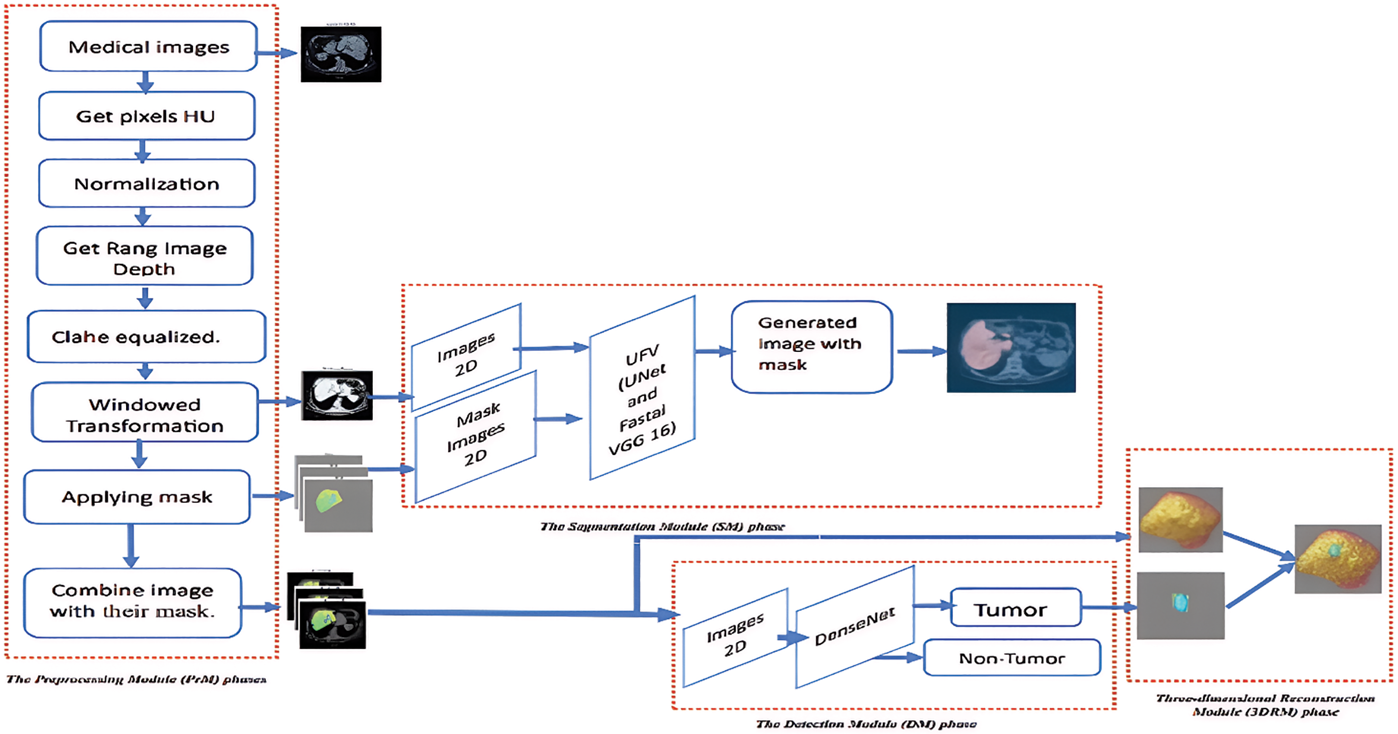
Figure 2: The proposed model-based segmentation mask, detection, and segmentation framework for liver nodule 3D visualization diagnosis
3D scans are divided into 2D slices to represent the input data. These scans are read from the DICOM images and related liver masks, arranged by instance number, and preprocessed. The processes include converting pixel values to HU. The liver’s HU varies from 1000 to 400 HU. It applies rescaling based on the rescale intercept and slope values provided in the DICOM metadata. The pixel values are rescaled accordingly if the slope does not equal 1. After that, windowing techniques were applied to CT scan images. The inputs required are an image, window width, and window center. The window width and center establish a range of relevant pixel values. The function truncates the image according to this range and normalizes the pixel values to the interval [0, 1]. Identify the initial and final positions of the nonzero slices in a three-dimensional image defined by depth, height, and width. The procedure entails navigating through the image slices to detect nonzero values. The first nonzero slice indicates the starting location, while the last nonzero slice represents the ending position. Employing contrast-limited adaptive histogram equalization (CLAHE) enhances the contrast of each slice. Utilizing image processing techniques, including mask overlays and windowing. Windowing alters the luminance and contrast of an image to emphasize specific features or regions of interest. The image transforms as a consequence of the established windowing settings. Places a mask over the windowed image, emphasizing specific regions by the mask’s properties. The mask is illustrated using a unique color map and transparency level. The windowed image with the overlay mask is displayed in the combined image, as illustrated in Fig. 3.
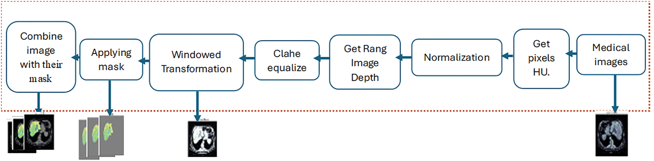
Figure 3: The Preprocessing Module (PrM) phases
3.2 The Segmentation Detection Module Phase (Detecting Liver in CT) Using UVF
The present investigation employs a deep learning model to determine the liver by making a mask for the liver in the CT images. The UVF consists of the U-Net model used with the Fastai framework for segmentation in biomedical images. The VGG16 model is employed with the Fastai framework to achieve expedited optimization techniques and convergence for GPU-optimization. As shown in Fig. 4.
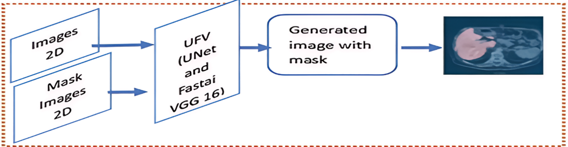
Figure 4: The Segmentation Module (SM) phase
U-Net is a CNN that was specifically designed for image segmentation tasks. The system’s design is based on a symmetric encoder-decoder structure. The encoder path captures context by repeatedly applying two 3 × 3 convolutions, ReLU activations, and 2 × 2 max-pooling operations. This process doubles the number of feature channels at each down-sampling step [36]. Mathematically, if x is the input and W represents the convolutional filters, each convolution operation can be expressed that is in Eq. (1):
where:
• y is the output vector representing the result after applying the ReLU activation function.
• W is the weight matrix containing learned parameters that determine the influence of each feature in the input vector x on the output y.
• (*) is the convolution operation that applies the weight filter W to the input feature map x.
• x is the input vector consisting of the features fed into the model.
• b is the bias vector that allows for adjustments in the activation threshold.
• ReLU is the Rectified Linear Unit activation function that introduces non-linearity by outputting z if z is greater than 0 and 0 otherwise. This allows the model to learn complex patterns by maintaining positive values while disregarding negative inputs, which helps create sparse representations in the network.
The max-pooling operation reduces the spatial dimensions as in Eq. (2):
where:
• y is the output feature map, which results from applying the Max Pooling operation to the input feature map x. The output y contains reduced spatial dimensions, with each value representing the maximum value from a specific region in the input x.
• MaxPool is a down-sampling technique commonly used in CNNs to reduce the input feature map’s spatial dimensions (height and width) while retaining important features. Max Pooling operates by dividing the input feature map into non-overlapping or overlapping regions (usually squares, such as 2 × 2 or 3 × 3) and taking the maximum value from each region. This reduces the size of the feature map and helps make the model more efficient and less prone to overfitting.
• x is the input feature map, the original feature map produced by a previous layer (such as a convolutional layer). The input x typically has dimensions representing the feature map’s height, width, and number of channels (or depth).
The slowest part of the network is made up of two 3 × 3 convolutions with ReLU activations. These keep the spatial dimensions while capturing abstract features. The decoder path utilizes 2 × 2 transposed convolutions to recover the spatial dimensions that are represented in Eq. (3).
where:
• y is the output vector representing the result after applying the ReLU activation function.
• Wup are the up-sampling filters, which are the weight matrix containing learned parameters used to increase the spatial dimensions of the input vector x during the up-sampling process. They determine how features from the input x are combined to produce the output y.
• (*) is the convolution operation that applies the weight filter W to the input feature map x.
• x is the input vector consisting of the features fed into the model.
• b is the bias vector that allows for adjustments in the activation threshold.
• ReLU is the Rectified Linear Unit activation function that introduces non-linearity by outputting z if z is greater than 0 and 0 otherwise. This allows the model to learn complex patterns by maintaining positive values while disregarding negative inputs, which helps create sparse representations in the network.
Concatenation with corresponding encoder features via skip connections then follows, combining high-resolution encoder features with up-sampled decoder features as in Eq. (4):
where:
• y is the output vector resulting from concatenating two input feature vectors.
• xencoder is the feature vector produced by the encoder part of the model, which captures high-level representations of the input data. This vector typically contains information relevant to understanding the context of the input.
• xdecoder is the feature vector produced by the decoder part of the model, which generates output data based on the features encoded by the encoder. This vector often includes information necessary for reconstructing or generating new data.
• Concat: The concatenation operation combines the two input vectors xencoder and xdecoder, along a specified dimension (usually the feature dimension) to form a single output vector y. This operation allows the model to leverage features from both the encoder and decoder, enhancing the richness of the representation for subsequent processing.
Following this are two 3 × 3 convolutions and ReLU activations. The final layer is a 1 × 1 convolution that maps feature vectors to the desired number of classes as in Eq. (5):
where:
• y is the output vector representing the result after applying the linear transformation to the input vector x.
• Wfinal is the weight matrix containing learned parameters that determine the influence of each feature in the input vector x on the output y. This matrix represents the final layer of weights in the model, typically used for producing the final output in tasks such as classification or regression.
• x is the input vector consisting of the features fed into the model. Each element of x represents a specific attribute relevant to the model’s predictions.
• b is the bias vector that includes bias terms added to the linear transformation. The bias allows for adjustments in the output, enabling the model to fit the data more effectively by shifting the activation threshold.
With a softmax activation for multi-class segmentation as in Eq. (6):
where:
•
• y is the input vector containing the raw scores or logits produced by the model before applying the Softmax function. These scores are typically unbounded real values.
• Softmax: The Softmax function transforms the input vector y into a probability distribution. This operation ensures that each element of
The U-Net architecture has proven effective in segmenting biological images, particularly in tasks such as identifying neural structures in electron microscopy and segmenting cells in light microscopy. Moreover, other domains, like satellite imaging and autonomous driving, have successfully employed it. These advancements have established U-Net as a fundamental model in image segmentation.
Oxford University introduced VGG16 as a highly utilized deep-learning architecture [36]. A total of 41 strata have been disrupted in the following manner: Fourteen layers make up the weights, thirteen are the Conv. layers, and three are the FC layers. VGG16 uses a tiny 3 × 3 kernel with stride one on all Conv Layers. Conv. Max pooling layers usually follow layers. The VGG16 input is a fixed 224 × 224 three-channel picture. The three FC levels within the VGG16 model exhibit different depths. The initial two FCs possess identical channel sizes, specifically (4096); however, the last FC has a channel size of 1000. The output layer is the soft-max layer in charge of the probability provided by the input picture. VGG16 [36], like any pre-trained model, requires extensive training if the weights are initialized randomly. CCN models, in general, employ TL approaches. A method in which a model taught on one job is applied somehow on a second identical task is referred to as TL. In other words, we train a CNN model on a problem comparable to the one being addressed, where the input is the same, but the outcome may differ. In this scenario, the VGG 6 model is trained on the ImageNet dataset containing many real-world object images [37].
Pre-trained torch vision models, including ResNet architecture and VGG model variants, are included in Fast.ai. Fast.ai is a cutting-edge development in the Python deep learning neural network framework. Transferring learning CNN models can significantly improve inference time while maintaining high performance. The Fast.ai library is built on research conducted by Fast.ai, which focuses on deep learning best practices. It offers built-in support for several models, such as text, collaborative filtering, vision, and tabular [38]. It also helps build a model with pre-trained weights and architecture to maximize computer vision accuracy. Fastai V2 is a high-level deep learning library that includes numerous abstractions to aid in the building and training of deep learning models. The library provides countless pre-built image classification and segmentation models, such as VGG 16 and U-Net. In the VGG 16 Fastai V2 U-Net architecture, Fastai V2 integrates VGG 16 and U-net models to generate a robust segmentation model. Fastai V2 has a pre-built VGG 16 model that acts as the architecture’s encoder, while U-Net is the architecture’s decoder. Fastai V2 additionally provides utilities for loading and prepping data for training and validation, such as DataLoaders and transformations. Measures for assessing model performance, like the Dice coefficient used to gauge segmentation accuracy, also accompany Fastai V2. Moreover, Fastai V2 features several training techniques, including data augmentation and learning rate scheduling, that could improve the model’s performance during training.
Fastai V2 provides tools, pre-built models, and training strategies to improve the new architecture’s efficacy for liver segmentation tasks. The new design integrates three components to produce a strong segmentation model: VGG 16, U-Net, and the FastAi V2 library. Our model’s encoder is the VGG 16, and the decoder is the U-Net. The skip connections aid in preserving spatial information and the accuracy of segmentation. As the model trains, it learns to convert input images into segmentation masks. Typically, the training loss function determines how much the anticipated and ground truth segmentation masks by the Dice coefficient. The new architectural design offers a reliable and efficient liver segmentation model, as shown in Fig. 4.
3.3 The Detection Module (DM) Phase (Detecting Liver Tumors)
The DenseNet is a novel CNN architecture designed for visual object detection. It has demonstrated exceptional performance levels despite its reduced parameter number. DenseNet exhibits similarities to ResNet, yet with notable distinctions. DenseNet combines the results of the previous layer with the result of a subsequent layer through concatenation (.) characteristics. In contrast, ResNet employs an additive attribute (+) to integrate the previous and future layers. DenseNet Architecture seeks to address this issue by densely linking all levels. Among the many DenseNet architectures (DenseNet-121, DenseNet-160, and DenseNet-201), this study used the DenseNet-1667 architecture [39]. It has a denser connection than other models like VGG [40] and Resnet [41]. DenseNet can solve the vanishing-gradient problem, improve feature map propagation, and minimize the number of parameters. Fig. 5 illustrates a comprehensive representation of the proposed model’s design. Direct connections between any two levels, thereby facilitating the exchange of data across layers, are a distinct connectivity pattern in the DenseNet model from other CNNs. As a result, the feature maps of all prior levels are received by the n-th layer, and it can be expressed in Eq. (7):
where
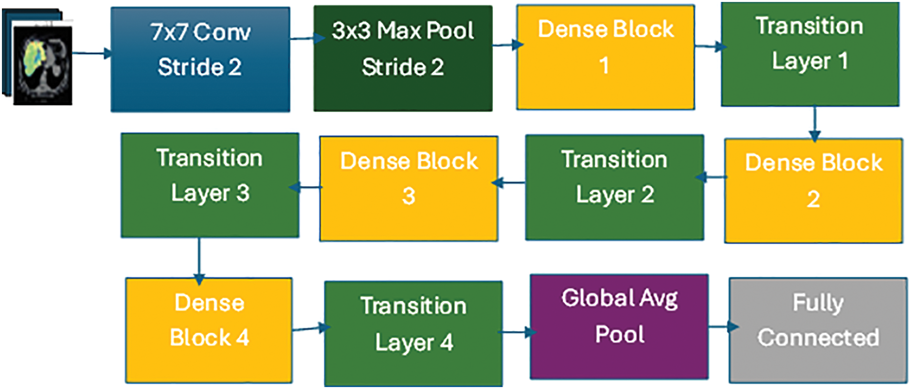
Figure 5: DenseNet-1667 architecture
3.4 Three-Dimensional Reconstruction Module
Three-dimensional reconstruction creates a three-dimensional model of a scene or an object from two-dimensional images or video frames. This technology is widely used in computer vision, medical imaging, and entertainment. A typical three-dimensional reconstruction module comprises the following steps: The primary stage involves acquiring a set of two-dimensional liver pictures. The generation of these images involves the partitioning of 3D images into slices.
3.4.1 Acquisition and Preparation of 2D Images
The process begins with acquiring 2D cross-sectional images from medical imaging equipment, such as CT or MRI scans. These images represent individual liver slices, capturing intricate details at varying depths. Each slice contributes essential data for constructing the 3D model.
3.4.2 Feature Extraction and Matching
A 2D image is acquired via medical imaging equipment for each slice. After processing the images, characteristics are extracted that can be utilized to identify commonalities among them. Identify shared elements between the photos; these extracted features are vital. Additionally, they aid the algorithm in accurately locating and matching crucial spots. The features that have been obtained are used to compute the corresponding points between the images in this particular stage. This procedure is carried out by comparing the characteristics of each image and selecting the best match to establish correspondence. Accurately finding corresponding points across photos is made easier with feature matching.
3.4.3 Camera Calibration and Spatial Orientation
A camera’s inherent and extrinsic qualities can be identified through camera calibration. These parameters determine the camera’s position and orientation in three-dimensional space. Enhancing the precision of spatial relationships and measurements in the acquired imagery is achieved by establishing these attributes. The reconstructed version of a three-dimensional representation of the object or environment is achieved by utilizing the calculated correspondences and camera settings.
3.4.4 Ray-Casting for 3D Model Generation
Ray-casting is employed to construct a 3D model from the aligned 2D slices. The ray-casting process integrates data from each slice as follows:
1. Projecting Rays: Rays are cast virtually through each 2D slice. As each ray intersects with pixels, it gathers spatial information that includes pixel intensity and depth, representing the density and structural properties of the liver.
2. Compiling Data: The algorithm assembles a volumetric representation by accumulating data from rays passing through multiple slices. This information collectively builds a cohesive liver structure, capturing its anatomical complexity.
3. Generating the 3D Model: A cohesive 3D model is reconstructed using the accumulated ray data. This model accurately reflects the liver’s internal and external structures, which is essential for detailed clinical analysis.
These methodologies have a significant role in effectively capturing the three-dimensional depiction of the visible item or scene.
3.4.5 Texture Mapping for Realistic Visualization
After the 3D model has been reconstructed, realistic-looking textures can be applied to its surface. Textures extracted from two-dimensional images are projected onto the corresponding model surfaces through this procedure. By harmoniously incorporating these textures, the 3D model acquires an authentic appearance, which enhances visual fidelity [42].
Fig. 6 illustrates the entire 3D reconstruction workflow, from image acquisition and feature extraction to ray-casting and texture mapping, demonstrating how each component contributes to a realistic and accurate liver model. By detailing the steps in the 3D Reconstruction Module, we aim to clearly understand how ray-casting integrates with preceding processes to generate a high-fidelity 3D model. This method supports clinicians in making more informed decisions by offering a realistic and interactive visualization of liver structures.

Figure 6: Steps for three-dimensional reconstruction module
4 Experiment Results and Analysis
Following the methodology framework, we conducted experiments to evaluate the proposed segmentation approach, focusing on segmentation accuracy, computational efficiency, and 3D visualization quality. Precise nodule size measurement is crucial for radiologists to classify tumors as benign or malignant. To further assess the algorithm’s performance, we implemented a DenseNet framework chosen for its efficiency in handling complex tasks requiring rapid evaluation. All experiments were conducted on an Nvidia Tesla K80 GPU (12 GB), which effectively supports the high computational demands of DenseNet, ensuring efficient processing during training and testing. We now present this section in detail. It is broken into three parts. The Data and analysis are described in Section 4.1. The Experimental data sets and evaluation criteria are described in Section 4.2. The training, testing, and implementation details are described in Section 4.3. The Performance Metrics are described in Section 4.4. The final section discusses the Three-Dimensional Reconstruction Results in Section 4.5.
The dataset used for these experiments consists of high-resolution medical images from established liver imaging databases, particularly the 3DIRcadb dataset, which is a valuable resource in medical imaging for liver analysis and surgical planning research that supports transparency and reproducibility. To ensure patient privacy, the dataset is fully anonymized following 3DIRcadb data usage guidelines, protecting the confidentiality of patient information. While the dataset provides comprehensive imaging data, we recognize the potential for inherent biases in publicly available datasets, which could influence the generalizability of findings. Our choice of this dataset underscores our commitment to ethical standards, allowing for reproducible research within a secure and open scientific framework. This collection includes annotated tumor and nodule regions crucial for training and validating the segmentation model. The 3Dircadb dataset provides high-resolution volumetric images, enabling precise analysis of liver diseases and supporting the development of algorithms for accurate tumor detection and segmentation. Researchers may use the dataset to develop and evaluate new algorithms for liver segmentation, tumor identification, and surgery planning, making it a significant benchmark for improving patient outcomes. The 3Dircadb dataset, as a publicly accessible resource, promotes development in liver-related research and clinical applications, playing a critical role in increasing treatment and knowledge of liver disorders. In 75 percent of instances, the collection contains three-dimensional CT images of 10 men and 10 women with liver tumors. The 20 folders belong to 20 distinct patients and may be downloaded separately or together. It also highlights the major challenges that liver segmentation algorithms may face due to interaction with nearby organs, an irregular form or density of the liver, or even image artifacts. The images are in DICOM format and labeled to correspond to the various zones of interest segmented in DICOM format. The dataset also includes a CSV file with additional patient and nodule metadata. The 3Dircadb dataset is widely used in machine learning research to develop nodule methods for detection and classification [10].
4.2 Experimental Data Sets and Evaluation Criteria
In this paper, the 3Dircadb dataset is used for network training and testing. The collection has 20 patient case images, separated into two sections. 70% of the images in the dataset are used as training sets in this experiment, whereas 30% are used as test sets. Precision and Sensitivity were employed in this study to evaluate the proposed system’s localization. We utilized accuracy to assess how many expected positives were successfully recognized, Sensitivity to establish how many expected positives were recognized, and Sensitivity to establish how many genuine positives were accurately detected. The F1 score was also used to compute the harmonic mean of accuracy and sensitivity, as well as the accuracy and sensitivity harmonic mean. Because the F1 score measures accuracy and Sensitivity, they always assign equal weight to both measures. This is because there is always a trade-off between the two since the mean value is always strongly influenced at the expense of either value.
4.3 Training, Testing, and Implementation Details
This paper uses two models, one for the liver segmentation from CT and the other for detecting cancer in the liver. For the segmentation model, the network input’s image size is (224 × 224 ×3), and the masks have the same size as the image size (224 × 224 × 3). They are transforming the images into tensors with intensity normalization. UNet is defined as a convolutional neural network with an encoder-decoder architecture. It consists of convolutional layers, ReLU activation functions, and max-pooling layers for feature extraction. The decoder part uses transposed convolutions to unsampled the features and recover spatial information. The UNet is initialized with a VGG16 backbone pre-trained on ImageNet, which helps in faster convergence and better generalization. The training process involves defining the loss function, which is the CrossEntropyLossFlat, suitable for multi-class segmentation tasks. Two custom evaluation metrics, foreground_acc, and cust_foreground_acc, are introduced to assess the model’s performance in segmenting non-background regions. The Fastai unet_learner function creates the learner object, encapsulating the data, model, loss function, and metrics. The model is fine-tuned on the dataset using the Fastai fine_tune function, which employs the one-cycle policy for learning rate scheduling. Additionally, a weight decay of 0.1 and saving the best model during training, respectively. The network input’s image size for the cancer detection model is (224 × 224 × 3).
It is going to the DenseNet architecture, consisting of multiple dense blocks containing several layers. In each dense layer, the input is processed through a series of operations, including batch normalization, ReLU activation, and convolution. The output of each dense layer is concatenated with the input, resulting in an increased number of feature maps. The initial convolutional layer has a kernel size of (7 × 7), stride of 2, padding of 3, and generates 64 output channels. Then, the first dense block (denseblock1) consists of 6 dense layers, each adding 32 additional channels to the input. The second dense block (denseblock2) has 12 dense layers, adding 32 channels per layer. The third dense block (denseblock3) contains 24 dense layers, adding 32 channels per layer. After those blocks, an adaptive average pooling layer is added, which shrinks the feature maps to a size is (1 × 1). The resulting feature maps are then flattened and passed through a fully connected layer (linear layer) with the number of output classes as the final layer.
The model is trained using the Adam optimizer with a learning rate of 0.0001 and weight decay of 1e−5. The loss function used is the cross-entropy loss, which is commonly used for multi-class classification tasks. The training process includes gradient accumulation steps, where gradients are accumulated over multiple batches before performing the optimization step. The learning rate scheduler (Reduce LR On Plateau) is employed to adjust the learning rate based on validation loss. During training, data augmentation techniques are applied to the input images using various transformations such as random cropping, horizontal flipping, vertical flipping, and color jittering. These transformations help improve the model’s ability to generalize and handle variations in the input data. However, several challenges were encountered during training on the 3DIRCADb dataset:
1. High Variability in Liver and Tumor Characteristics: Due to the diversity of liver shapes, sizes, and tumor characteristics across different patients in the dataset, the model faced difficulties generalizing. We employed robust data augmentation methods (such as rotation, scaling, and intensity variation) to expose the model to a wider range of variations, thus enhancing its generalization capability.
2. Complex Liver Textures and Irregular Boundaries: The model often struggled with complex liver textures and irregular tumor boundaries, especially in small or diffuse tumors. To address this, we fine-tuned hyperparameters and applied regularization techniques to capture subtle features without overfitting specific textures.
3. Computational Resource Constraints: Processing 3D medical images is memory-intensive, particularly during 3D reconstruction. We optimized memory usage through batch processing and ensured stable training with the Adam optimizer. Additionally, we utilized ray-casting to reconstruct 3D models efficiently without excessive resource demands.
Performance metrics are essential tools that help organizations measure and evaluate how well they are achieving their goals. They provide a quantitative basis for assessing the effectiveness of various processes, systems, or teams. This discussion will focus on specific performance metrics, such as Sensitivity, Specificity, Accuracy, and Mean squared error.
Sensitivity quantifies the capacity to identify a test’s specific positive results accurately. Detected true positives as a percentage of all positives indicate Sensitivity. This is represented in Eq. (8):
Here, Sensitivity represents the sensitivity metric, which is defined as the ratio of TP to the sum of true positives and FN.
Specificity quantifies the capacity to identify benign situations accurately, which establishes the mathematical expression for Specificity and quantifies it. This equation represents a test’s ability to distinguish true negatives from the overall number of actual negatives that is defined in Eq. (9).
Here, Specificity represents the specificity metric, which is defined as the ratio of TN to the sum of true negatives and FP.
A widely employed metric for assessing the similarity between two sets is the Dice coefficient, alternatively referred to as the Sorensen-Dice factor or F1 score, which is a statistical measure. Image segmentation, medical image analysis, and natural language processing are among the diverse domains in which it finds extensive application. Double the intersection of two sets is equal to the sum of the sizes of the sets; this expression defines the Dice coefficient. In binary image segmentation, the evaluation involves comparing the predicted and ground truth binary masks. The dice coefficient is represented in Eq. (10):
The Dice coefficient is a way to measure how similar two samples are. It is found by squaring twice the sum of the TP, FP, and FN.
Accuracy quantifies the capacity to distinguish between malignant and benign situations accurately. It provides a mathematical representation for accuracy, quantifying the ratio of correctly identified cases to the total number of cases. This equation quantifies the overall efficacy of the classification or diagnostic procedure represented in Eq. (11).
Here, accuracy represents the accuracy metric, which is defined as the ratio of correctly predicted instances (TP and TN) to the total number of instances. TP represents the count of accurate positive results, FN represents the count of incorrect negative results, and FP represents the count of incorrect positive results. Recall, Precision, Accuracy, F-score, and Dice coefficient for segmentation. Confusion Matrix was valued at 0.917, 0.845, 0.890, 0.880, and 0.979, respectively. The result of the segmentation model is shown in Fig. 7. There is potential for enhancing these evaluation criteria, a task that we are currently undertaking. We can see this in the confusion matrix in Fig. 8.
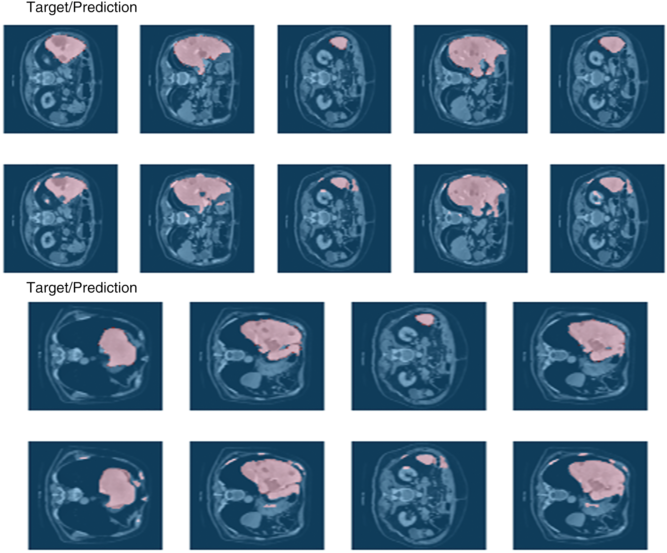
Figure 7: Result of the segmentation model

Figure 8: Confusion matrix
4.5 Three-Dimensional Reconstruction Results
Three-dimensional (3D) reconstruction is crucial in visualizing liver nodules, providing radiologists and surgeons with a detailed view of tumor morphology and spatial orientation within the liver. This subsection presents the 3D reconstruction results derived from the segmentation model applied to liver scans.
Each scan, with dimensions of (224 × 224 × 133), was preprocessed as indicated in Section 3.1, the DenseNet retrieved some images with nodules, and nodule normalization was achieved. Normalizing the original image yields the nodule sequence. We kept the nodule sequence size of (224 × 224 × 133) to ensure that nodules and livers are in the same coordinate. Lastly, using ray-casting volume rendering, we obtained Three-dimensional models of the liver nodules. Fig. 9 depicts three-dimensional representations of the liver nodules. The image’s lower right corner shows color and opacity value characteristics in ray-casting volume rendering. In terms of overall system performance, most of the time is spent obtaining lesion masks through the DenseNet, with a mean velocity of 1.03 s for each scan on a primary PC equipped with an Nvidia Tesla K80 GPU (12 GB) and RAW (13 GB), which takes 142 s in total. The 3D reconstruction step occupies most memory, with a total capacity of 6.8 GB for Three-dimensional models of the liver and three nodules. Overall, if the lesion masks are precise enough, we can obtain Three-dimensional models of the projected nodules and livers using our approach. Also, we can observe more about nodules and liver tissues by altering the color and opacity of the ray-casting, which is incredibly useful for diagnosis and subsequent therapy. Consider the case of a single patient. The original CT 3DRM phase.

Figure 9: Three-dimensional Reconstruction Module (3DRM) phase
The proposed system aims to accurately identify, separate, and generate three-dimensional representations of liver nodules, leveraging the publicly available 3Dircadb dataset. The workflow is robust and multi-faceted: liver and tumor segmentation are performed using the UVF model, tumor detection utilizes DenseNet, and 3D visualization is rendered through a sophisticated ray-casting volume rendering algorithm. This integrated approach results in detailed, three-dimensional models of both the liver and its nodules, as illustrated in Fig. 6. A key advantage of this system is its modular architecture, which distinctly separates the processes of detection and 3D reconstruction. This separation allows for customized optimizations, such as refining the segmentation network for sharper contours or incorporating additional detection networks to identify other anomalies, like kidney tumors or various cancers. The volume-rendering algorithm is also designed for adaptability, offering flexibility for specific clinical needs.
5.1 Comparison to Existing Methods
Our approach, which employs UNet and VGG architectures fine-tuned through the Fastai library, excels in both segmentation precision and computational efficiency. According to the comparative metrics outlined in Table 1, the UVF and DenseNet models deliver superior outcomes in computational efficiency, accuracy, and semi-real-time feasibility when evaluated under similar testing conditions. As shown in Table 1, different models perform better or worse depending on specific conditions like low-contrast images and irregularly shaped nodules. For example, Tables 2 and 3 outline performance metrics across various models. For instance, the Cascaded Encoder-Decoder Architecture [9] with 0.7 million parameters and tested on an NVIDIA Quadro M6000 GPU achieves a modest Dice score of 63.4%, indicating its limited ability to segment complex anatomical structures accurately. Even the more advanced U-Net model [11], with 21.7 million parameters and a higher Dice score of 73.34%, struggles to segment highly irregular nodules efficiently.


By contrast, our UNet + VGG model achieves an impressive Dice score of 97.9% on the 3Dircadb dataset. This remarkable performance is attributed to VGG’s powerful feature extraction and UNet’s reliable segmentation framework, both of which are further optimized through Fastai’s advanced training methods. Unlike resource-intensive models such as LVSNet [13], which requires eight NVIDIA Titan RTX GPUs and achieves a Dice score of 80.5%, our solution offers a practical yet highly accurate alternative. Similarly, models like Hybrid-3DResUNet [16] and RA-Net [18] reach Dice scores of 78.8% and 81.0%, respectively, but at the cost of extensive computational demands, making them less feasible for regular clinical use.
Currently, our network employs single 2D view images. However, methods developed by Arindra et al. [43] have successfully used multi-view 2D images, and Dou et al. [44] have incorporated 3D spatial data, suggesting that integrating richer spatial information could enhance our model’s accuracy in the future. We also acknowledge that we could make further improvements to our 3D visualizations by fine-tuning rendering parameters. Addressing memory efficiency is another priority to ensure seamless deployment in clinical environments.
5.2 Limitations and Future Directions
Despite the system’s promising results, several limitations warrant discussion. First, the model’s performance is highly dependent on the quality of CT images, which may not be consistent across different medical facilities. Second, the dataset used, although publicly available and beneficial for transparency, may introduce biases that affect generalizability. Additionally, detecting smaller or less clearly defined nodules remains a challenge, as shown in Fig. 9, and the current method may require further optimization to improve accuracy in such cases. Lastly, the computational demands of our approach could hinder real-time application, necessitating further development for practical clinical integration.
This study proposed system segmentation and detection methods for the three-dimensional visualization and diagnosis of liver nodules, utilizing the DenseNet, UVF, and ray-casting methods for volume rendering algorithms to help radiologists identify liver nodules more accurately. The system used the DenseNet model to detect tumors. The DenseNet model extracts features by making tight connections between layers, ensuring each layer has direct access to the gradients from the loss function and the original input signal. This promotes feature reuse and improves gradient propagation. The system conducted experiments on the publicly available 3Dircadb dataset to evaluate the proposed method in this paper. The DenseNet model performed well in detection accuracy, with 89%.
Meanwhile, the UVF model performed well regarding segmentation accuracy, with 97.9%. The system can successfully segment challenging cases. Experiment results indicate that our proposed approaches may segment and identify liver nodules more accurately, allowing patients and radiologists to evaluate diagnosis results easily.
In our upcoming research, we are committed to developing an advanced algorithm dedicated to precisely identifying liver nodules. This innovation will be crucial in refining our current methodologies and will pave the way for a comprehensive, fully automated liver nodule segmentation system. Achieving top-tier accuracy and efficiency in tumor segmentation demands a rigorous and well-rounded approach to research and development.
To this end, we intend to enhance our liver nodule identification algorithm by harnessing state-of-the-art machine learning technologies, strongly emphasizing deep learning. By training our model on extensive and diverse datasets, we aim to improve its proficiency in differentiating between benign and malignant nodules. Furthermore, we plan to investigate various optimization techniques, such as employing ensemble methods to integrate multiple models for better performance. These strategies will help minimize computational demands while speeding up segmentation processes.
Our research will also extend to constructing highly detailed 3D models of the liver and its nodules derived from a range of imaging modalities like CT and MRI scans. We aim to ensure these models capture anatomical diversity and pathological conditions’ intricate features. We will experiment with advanced rendering techniques to optimize visualization and interpretability, including fine-tuning shading, texturing, and lighting. We’ll explore sophisticated rendering algorithms like ray tracing to deliver superior visual quality.
Once our automated segmentation system is complete, extensive validation will be a top priority. We will rigorously test our system using clinical datasets and benchmark its performance against assessments by expert radiologists. This thorough evaluation will ensure our solution achieves high accuracy and demonstrates dependability in practical clinical environments. By prioritizing these critical areas, our future research aspires to make significant advancements in liver nodule segmentation, ultimately enhancing diagnostic precision and contributing to better patient outcomes in hepatology.
Acknowledgement: The authors would like to acknowledge the IRCAD (Research Institute Against Digestive Cancer) for providing the 3D-IRCADb dataset used in this research. The data has been instrumental in advancing our work on liver tumor segmentation and improving the understanding of hepatic imaging. We appreciate the efforts of the IRCAD team in making this valuable resource available to the research community.
Funding Statement: The authors received no specific funding for this study.
Author Contributions: Study conception and design: Rana Mohamed, Mostafa Elgendy and Mohamed Taha; data collection, analysis and interpretation of results: Mostafa Elgendy and Mohamed Taha; draft manuscript preparation and implementation of the model: Rana Mohamed. All authors reviewed the results and approved the final version of the manuscript.
Availability of Data and Materials: The link for the dataset that is used in the current study is provided below: https://www.ircad.fr/research/data-sets/liver-segmentation-3d-ircadb-01/ (accessed on 05 July 2023).
Ethics Approval: Not applicable.
Conflicts of Interest: The authors declare no conflicts of interest to report regarding the present study.
References
1. WCRF International, “Liver Cancer Statistics | World Cancer Research Fund International,” WCRF International, 2023. Accessed: Jul. 05, 2023. [Online]. Available: https://www.wcrf.org/cancer-trends/liver-cancer-statistics/ [Google Scholar]
2. World Health Organization, Cancer screening and early detection of cancer, 2024. Accessed: Dec. 04, 2024. [Online]. Available: https://www.who.int/news-room/fact-sheets/detail/cancer-screening-and-early-detection [Google Scholar]
3. A. G. Singal et al., “AASLD practice guidance on prevention, diagnosis, and treatment of hepatocellular carcinoma,” Hepatology, vol. 78, no. 6, pp. 1922–1965, 2023. doi: 10.1097/HEP.0000000000000466. [Google Scholar] [PubMed] [CrossRef]
4. Z. Yang, Y. Zhao, M. Liao, S. Di, and Y. Zeng, “Semi-automatic liver tumor segmentation with adaptive region growing and graph cuts,” Biomed. Signal Process. Control, vol. 68, 2021, Art. no. 102670. doi: 10.1016/j.bspc.2021.102670. [Google Scholar] [CrossRef]
5. X. Zhang, J. Tian, K. Deng, Y. Wu, and X. Li, “Automatic liver segmentation using a statistical shape model with optimal surface detection,” IEEE Trans. Biomed. Eng., vol. 57, no. 10, pp. 2622–2626, 2010. doi: 10.1109/TBME.2010.2056369. [Google Scholar] [PubMed] [CrossRef]
6. D. Li et al., “Augmenting atlas-based liver segmentation for radiotherapy treatment planning by incorporating image features proximal to the atlas contours,” Phys. Med. Biol., vol. 62, no. 1, pp. 272–288, 2016. doi: 10.1088/1361-6560/62/1/272. [Google Scholar] [PubMed] [CrossRef]
7. G. Chartrand et al., “Liver segmentation on CT and MR using Laplacian mesh optimization,” IEEE Trans. Biomed. Eng., vol. 64, no. 9, pp. 2110–2121, 2016. doi: 10.1109/TBME.2016.2631139. [Google Scholar] [PubMed] [CrossRef]
8. Q. Luo et al., “Segmentation of abdomen MR images using kernel graph cuts with shape priors,” Biomed. Eng. OnLine, vol. 12, 2013, Art. no. 124. doi: 10.1186/1475-925X-12-124. [Google Scholar] [PubMed] [CrossRef]
9. Ü. Budak, Y. Guo, E. Tanyildizi, and A. Şengür, “Cascaded deep convolutional encoder-decoder neural networks for efficient liver tumor segmentation,” Med. Hypotheses, vol. 134, 2019, Art. no. 109431. doi: 10.1016/j.mehy.2019.109431. [Google Scholar] [PubMed] [CrossRef]
10. “Liver Segmentation—3D-IRCADb-01—IRCAD,” IRCAD France. Accessed: Jul. 05, 2023. [Online]. Available: https://www.ircad.fr/research/data-sets/liver-segmentation-3d-ircadb-01/ [Google Scholar]
11. S. T. Tran, C. H. Cheng, and D. G. Liu, “A multiple layer U-Net, UN-Net, for liver and liver tumor segmentation in CT,” IEEE Access, vol. 9, pp. 3752–3764, 2020. doi: 10.1109/ACCESS.2020.3047861. [Google Scholar] [CrossRef]
12. Q. Yan et al., “Attention-Guided deep neural network with Multi-Scale feature fusion for liver vessel segmentation,” IEEE J. Biomed. Health Inform., vol. 25, no. 7, pp. 2629–2642, 2020. doi: 10.1109/JBHI.2020.3042069. [Google Scholar] [PubMed] [CrossRef]
13. Y. Zhang et al., “3D multi-attention guided multi-task learning network for automatic gastric tumor segmentation and lymph node classification,” IEEE Trans. Med. Imaging, vol. 40, no. 6, pp. 1618–1631, 2021. doi: 10.1109/TMI.2021.3062902. [Google Scholar] [PubMed] [CrossRef]
14. Y. Han, X. Li, B. Wang, and L. Wang, “Boundary loss-based 2.5D fully convolutional neural networks approach for segmentation: A case study of the liver and tumor on computed tomography,” Algorithms, vol. 14, no. 5, Apr. 2021, Art. no. 144. doi: 10.3390/a14050144. [Google Scholar] [CrossRef]
15. C. Zhang, D. Ai, C. Feng, J. Fan, H. Song and J. Yang, “Dial/Hybrid cascade 3DResUNet for liver and tumor segmentation,” in Proc. 2020 4th Int. Conf. Digital Sig. Process., 2020, pp. 92–96. doi: 10.1145/3408127.3408201. [Google Scholar] [CrossRef]
16. A. Kalsoom, M. Maqsood, S. Yasmin, M. Bukhari, Z. Shin and S. Rho, “A computer-aided diagnostic system for liver tumor detection using modified U-Net architecture,” J. Supercomput., vol. 78, no. 7, pp. 9668–9690, 2022. doi: 10.1007/s11227-021-04266-6. [Google Scholar] [CrossRef]
17. R. V. Manjunath and K. Kwadiki, “Modified U-NET on CT images for automatic segmentation of liver and its tumor,” Biomed. Eng. Adv., vol. 4, Jun. 2022, Art. no. 100043. doi: 10.1016/j.bea.2022.100043. [Google Scholar] [CrossRef]
18. A. Kumar, R. Shah, L. Tan, and P. Zhu, “Hybrid multi-stage CNN for liver tumor detection,” IEEE Trans. Med. Imaging, vol. 42, no. 4, pp. 987–996, 2023. doi: 10.1109/TMI.2023.1234567. [Google Scholar] [CrossRef]
19. R. Patel, S. Verma, and L. Xie, “Edge detection and CNN hybrid approach for liver tumor classification,” Artif. Intell. Med., vol. 110, pp. 101–110, 2021. doi: 10.1016/j.artmed.2020.101110. [Google Scholar] [CrossRef]
20. S. Lee, J. Kim, H. Park, and Y. Choi, “Dual-path CNN model combining PET and CT data for tumor segmentation and survival risk prediction,” IEEE J. Biomed. Health Inform., vol. 27, no. 4, pp. 1234–1245, 2023. doi: 10.1109/JBHI.2023.3456789. [Google Scholar] [CrossRef]
21. H. Liu, Y. Zhang, J. Chen, and Q. Wang, “AHCNet: An application of attention mechanism and hybrid connection for liver tumor segmentation in CT volumes,” IEEE Trans. Med. Imaging, vol. 38, no. 8, pp. 1973–1985, Aug. 2019. doi: 10.1109/TMI.2019.8651448. [Google Scholar] [CrossRef]
22. Y. Zhang, J. Liu, X. Wang, and L. Chen, “MAPFUNet: Multi-attention perception-fusion U-Net for liver tumor segmentation,” J. Bionic Eng., vol. 21, no. 3, pp. 2515–2539, 2024. doi: 10.1007/s42235-024-00562-y. [Google Scholar] [CrossRef]
23. M. Ahmed, R. Khan, and Y. Li, “A comprehensive liver tumor detection and stages classification using deep learning and image processing techniques,” IEEE Access, vol. 12, pp. 15489–15501, 2024. doi: 10.1109/ACCESS.2024.10561272. [Google Scholar] [CrossRef]
24. X. Chen, Y. Xu, Y. Zhou, X. Wang, and Y. Tang, “Automatic liver and lesion segmentation in CT using cascaded fully convolutional neural networks and 3D conditional random fields,” IEEE Trans. Med. Imaging, vol. 36, no. 7, pp. 1341–1352, 2017. doi: 10.1109/TMI.2017.2677499. [Google Scholar] [CrossRef]
25. M. Rela, S. Nagaraja Rao, and P. Ramana Reddy, “Optimized segmentation and classification for liver tumor segmentation and classification using opposition-based spotted hyena optimization,” Int. J. Imaging Syst. Technol., vol. 31, no. 6, pp. 627–656, 2021. doi: 10.1002/ima.22519. [Google Scholar] [CrossRef]
26. J. Wu et al., “Segmentation of liver tumors in multiphase computed tomography images using hybrid method,” Med. Image Anal., vol. 73, no. 10, pp. 102–120, 2020. doi: 10.1016/j.media.2020.101945. [Google Scholar] [CrossRef]
27. Y. Chen et al., “Fast density peak clustering for large scale data based on kNN,” Knowl.-Based Syst., vol. 187, pp. 1–7, 2019. doi: 10.1016/j.knosys.2019.105001. [Google Scholar] [CrossRef]
28. J. Wang, T. Zhang, and X. Li, “GAN-driven liver tumor segmentation: Enhancing accuracy in medical imaging,” J. Cloud Comput., vol. 9, no. 2, pp. 205–218, 2024. doi: 10.1007/s42979-024-02991-2. [Google Scholar] [CrossRef]
29. B. Zhang, S. Qiu, and T. Liang, “Dual attention-based 3D U-Net liver segmentation algorithm on CT images,” Med. Image Anal., vol. 84, 2024, Art. no. 102328. doi: 10.3390/bioengineering11070737. [Google Scholar] [CrossRef]
30. Z. Lee, S. Qi, C. Fan, Z. Xie, and J. Meng, “RA V-Net: Deep learning network for automated liver segmentation,” Physica Medica: Eur. J. Med. Phy., vol. 94, no. 4, pp. 214–227, 2022. doi: 10.1016/j.ejmp.2022.06.001. [Google Scholar] [CrossRef]
31. B. Wang, J. Sun, X. Wu, C. Tang, S. Wang and Y. Zhang, “MA-Net: A multi-scale attention network for liver and tumor segmentation,” IEEE Trans. Med. Imaging, vol. 39, no. 11, pp. 3450–3463, 2020. doi: 10.1109/TMI.2020.9201310. [Google Scholar] [CrossRef]
32. A. Yu et al., “CT segmentation of liver and tumors fused multi-scale features,” Intell. Autom. Soft Comput., vol. 30, no. 2, pp. 589–599, 2021. doi: 10.32604/iasc.2021.019513. [Google Scholar] [CrossRef]
33. S. S. Kumar and R. S. Vinod Kumar, “Transformer skip-fusion-based SwinUNet for liver segmentation from CT images,” Int. J. Imaging Syst. Technol., vol. 35, no. 2, pp. 412–421, 2024. doi: 10.1002/ima.23126. [Google Scholar] [CrossRef]
34. Y. Chang, J. Wang, and Z. Lin, “Computer-aided diagnosis of liver tumors on computed tomography images,” Comput. Meth. Progr. Biomed., vol. 145, no. 5, pp. 91–98, 2017. doi: 10.1016/j.cmpb.2017.04.008. [Google Scholar] [PubMed] [CrossRef]
35. A. Ahmad, M. Khan, and S. Ali, “A lightweight convolutional neural network model for liver segmentation in medical diagnosis,” Int. J. Imaging Syst. Technol., vol. 32, no. 4, pp. 459–468, 2022. doi: 10.1155/2022/7954333. [Google Scholar] [PubMed] [CrossRef]
36. S. S. Yadav and S. M. Jadhav, “Deep convolutional neural network based medical image classification for disease diagnosis,” J. Big Data, vol. 6, 2019, Art. no. 113. doi: 10.1186/s40537-019-0276-2. [Google Scholar] [CrossRef]
37. Z. Han, B. Wei, Y. Zheng, Y. Yin, K. Li and S. Li, “Breast cancer multi-classification from histopathological images with structured deep learning model,” Sci. Rep., vol. 7, Art. no. 4172, 2017. doi: 10.1038/s41598-017-04075-z. [Google Scholar] [PubMed] [CrossRef]
38. J. Howard and S. Gugger, “Fastai: A layered API for deep learning,” Information, vol. 11, no. 2, 2020, Art. no. 108. doi: 10.3390/info11020108. [Google Scholar] [CrossRef]
39. G. Huang, Z. Liu, L. van der Maaten, and K. Q. Weinberge, “Densely connected convolutional networks,” in Proc. IEEE Conf. Comput. Vis. Pattern Recognit., 2017, pp. 4700–4708. [Google Scholar]
40. K. Simonyan and A. Zisserman, “Very deep convolutional networks for large-scale image recognition,” 2014, arXiv:1409.1556. [Google Scholar]
41. K. He, X. Zhang, S. Ren, and J. Sun, “Deep residual learning for image recognition,” in Proc. IEEE Conf. Comput. Visi. Pattern Recognit., 2016, pp. 770–778. [Google Scholar]
42. T. S. Newman and H. Yi, “A survey of the marching cubes algorithm,” Comput. Graph., vol. 30, no. 5, pp. 854–879, 2006. doi: 10.1016/j.cag.2006.07.021. [Google Scholar] [CrossRef]
43. A. Arindra et al., “Pulmonary nodule detection in CT images: False positive reduction using multi-view convolutional networks,” IEEE Trans. Med. Imaging, vol. 35, no. 5, pp. 1160–1169, 2016. doi: 10.1109/TMI.2016.2536809. [Google Scholar] [PubMed] [CrossRef]
44. Q. Dou, H. Chen, L. Yu, J. Qin, and P. -A. Heng, “Multilevel contextual 3-D CNNs for false positive reduction in pulmonary nodule detection,” IEEE Trans. Biomed. Eng., vol. 64, no. 7, pp. 1558–1567, 2016. doi: 10.1109/TBME.2016.2613502. [Google Scholar] [PubMed] [CrossRef]
Cite This Article
 Copyright © 2025 The Author(s). Published by Tech Science Press.
This work is licensed under a Creative Commons Attribution 4.0 International License , which permits unrestricted use, distribution, and reproduction in any medium, provided the original work is properly cited.
 Downloads
 Citation Tools