SPQ: An Improved Q Algorithm Based on Slot Prediction

1  Introduction

Radio Frequency Identification (RFID) [1] originated from the research of radar technology in the 1940s, non-contact two-way data communication is carried out through radio frequency, and recording media such as electronic tags are read and written to achieve the purpose of identifying targets or data exchange.

Typically, an RFID [2–4] system comprises components such as an antenna, Reader, and personal computer. It achieves data communication between the Reader and tags using wireless radio frequency, enabling data exchange.

Compared to traditional methods, RFID offers several advantages, including non-contact operation, high read efficiency, resistance to wear, strong anti-interference capabilities, and extended lifespan. When supported by anti-collision algorithms, readers can prevent collisions among targets and simultaneously recognize multiple tags.

To this day, RFID has been widely applied in various fields such as logistics, transportation, identity recognition, and information statistics. Examples include cargo tracking, management of bus hubs, and ID card recognition. As the number of applications grows, a challenge in RFID development lies in mitigating the impact on data read efficiency caused by multiple tag collisions. Specifically, optimizing RFID anti-collision algorithms to enhance work efficiency becomes more and more crucial [5,6].

Currently, random algorithms based on ALOHA due to simplicity, practicality, and cost-effectiveness, have seen more widespread adoption. Over the years, this algorithm has undergone continuous improvement, evolving from Pure ALOHA (PA) to Slotted ALOHA (SA), Framed Slotted ALOHA (FSA), and Dynamic Framed Slotted ALOHA (DFSA). Most commercial readers now employ the Q algorithm specified by the Electronic Product Code Global Class1 Generation2 (EPC Global C1 G2) standard [7], which belongs to the category of random algorithms. In recent years, the academic community has proposed several enhancements to the Q algorithm. For instance, Threshold Grouping Dynamic Q (TGDQ) [8] introduced two c parameters, c1 and c2, and the double parameters are dynamically adjusted with the change of Q value. FastQ [9] dynamically adjusts the optimal frame length based on the no-collision ratio of the slot. Subset Enhanced Performance-Q (SUBEP-Q) [10] leverages the concept of subframes and system efficiency priority to rapidly estimate the number of tags and dynamically adjust frame length after each subframe identification.

This paper proposes a dynamic Q value optimization algorithm based on Vogt-II slot prediction [11,12], incorporating Markov chains [13–15] and Whale Optimization Algorithm (WOA) [16–19]. Importantly, the algorithm is fully compatible with the EPC Global C1 G2 standard, which improves the throughput of the RFID system while ensuring practicality and compatibility.

2  System Model of RFID

As is shown in Fig. 1, a Radio Frequency Identification (RFID) system consists of an RFID antenna, RFID Reader, and personal computer. The RFID Reader is an IoT device, which reads and identifies the tag.

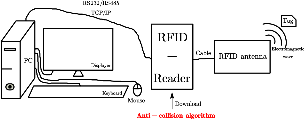
Figure 1: Diagram of a RFID system with computer, reader and antenna

When a tag is in proximity, the RFID antenna senses it through electromagnetic waves and transmits the tag information to the RFID reader via a cable. The RFID reader interprets the tag information. Successful identification occurs only when a single tag information is processed at any given time. The processed information is then transmitted to a personal computer through either the RS232/RS485 communication interface or the TCP/IP protocol. However, when multiple tags appear at the same time around the electromagnetic wave radiated by the RFID antenna, there will be multiple tag information at the same time processed by the RFID Reader, and information collision will occur. Therefore, to reduce the probability of the above situation, the anti-collision algorithm will be downloaded in the RFID Reader to improve the probability of successful identification, and then improve the throughput of the system.

3  Analysis of Q Algorithm

This section mainly introduces the principle of Q algorithm and summarizes the defects.

3.1 Principle of Q Algorithm

Electronic Product Code Global Class1 Generation2 (EPC Global C1 G2) uses a step parameter C and a floating-point number Qfp in Q algorithm. The C is used to dynamically adjust Qfp and it ranges from 0.1 to 0.5. The Q value is the result of rounding Qfp and it ranges from 0 to 15. The relationship between frame length N and Q value is shown in Eq. (1):

N=2Q(1)

The reader first sends the initial Q value, that is the initial frame length, and the tag to be read generates a random number within the frame length [0, 2Q− 1] and stores it in the slot counter. Each time, the reader only reads the tag whose slot counter is 0, so there are three situations when the information is read.

(1)   No tag information is received, that is, the slot is empty, so the Q value should be reduced.

(2)   A tag message is received, that is, the reading is correct, so that the Q value is unchanged.

(3)   Multiple tag information is received, that is, a collision occurs at this read, so the Q value must be increased.

When the Q value is large, the C is small, and when the Q value is small, the C is large. If the Q value changes after each read, the current frame needs to be ended, so that each tag generates a random number according to the new Q value. If the tag is read successfully, the next slot is continued, and the slot counter of the tag to be read is reduced by one, and the cycle is repeated. The algorithm flow is shown in Fig. 2.

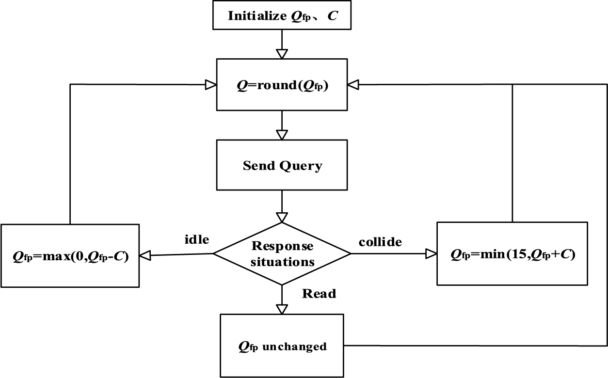
Figure 2: Flowchart of traditional Q algorithm

3.2 Q Algorithm Summary

Q algorithm adjusts the frame length by step C in real-time. However, when only the current slot is referenced, the direct adjustment of the Q value will cause the frame length to change too much, resulting in too many idle slots and collision slots. In addition, when the actual number of tags differs too much from the current Q value, the adjustment time is too long, which affects the system’s efficiency.

4  Improved Q Algorithm Based on Vogt-II

This section mainly aims at defects of Q algorithm and proposes a scheme based on the Vogt-II prediction algorithm, which combines the Markov decision chain and the Whale Optimization Algorithm (WOA).

4.1 Basis of Algorithm

4.1.1 Frame Length Determination Principle

In the stochastic ALOHA algorithm, assuming that the frame length is N, the number of tags to be identified is n, and the tag randomly selects a number within the frame length is equivalent to the binomial distribution model, then the expected number of slots for r tags to be successfully read within a frame is shown in Eq. (2):

αrN,n=N⋅Cnr(1N)r(1−1N)n−r(2)

When r is 0, 1, and a number greater than 1, it can represent the situation of slot idle, read, and collision, and the expectations are shown in Eq. (3):

α0N,n=N(1−1N)nα1N,n=n(1−1N)n−1αiN,n=N−α0N,n−α1N,n(3)

The throughput rate of the system is shown in Eq. (4):

S=α1N,nN=nN⋅(1−1N)n−1(4)

By solving Eq. (3), we can find that the throughput can reach the theoretical maximum when the frame length is consistent with the number of tags.

4.1.2 Vogt-II Prediction Principle

Vogt-II algorithm, also known as the Chebyshev inequality algorithm, predicts the number of remaining tags based on the identified slot conditions. Vogt-II algorithm has the advantage of making full use of the identification conditions and is more rapid and accurate than the traditional Q value adjustment frame length mechanism. Combining the Vogt-II prediction algorithm with the traditional Q algorithm can effectively make up for the shortcomings.

The actual recognition situation in a frame and the expected recognition situation in Eq. (3) is respectively composed of two vectors, which are shown in Eq. (5):

δ1=(c0,c1,ci)Tδ2=(α0,α1,αi)T(5)

The space distance D between the two vectors is shown in Eq. (6):

D=min|δ2−δ1|(6)

The number of remaining tags is predicted by the minimum spatial distance of the two vectors to obtain the minimum error. In general, to determine the number of tags in the response range of the reader, the number of tags is selected in the interval [c1+2ci,2×(c1+2ci)] to calculate D. At this point, the number of tags to be identified is: location(D)+c1+2ci, location(D) is the selection of the number of tags when the space distance is minimum.

4.1.3 Markov Decision Chain Optimization x-Q Relationship

In the Dynamic Framed Slotted ALOHA (DFSA) algorithm, Vogt-II predicts the recognition of a frame with a fixed value, and to combine it with Q algorithm, the idea of Markov decision chain is added based on the key problem of how to better value the number of identified slots.

The Markov chain is a statistical model based on random processes, and its core property is memoryless, that is the next state of the system is only related to the current state. The sum of each row element of the Markov chain’s state transition matrix is 1, and such matrix is called the probability transition matrix. The state transition matrix of the Markov chain can be used to represent the probability of state transition. Taking a group of slot recognition conditions as the state of a time point, the influence of slot number on the prediction accuracy of Vogt-II is analyzed by the state transition probability matrix.

In this paper, the optimal x-Q relationship is obtained by comparing the adjustment conditions of slot free rate and collision rate under different packet slot number x, and the model diagram is shown in Fig. 3.

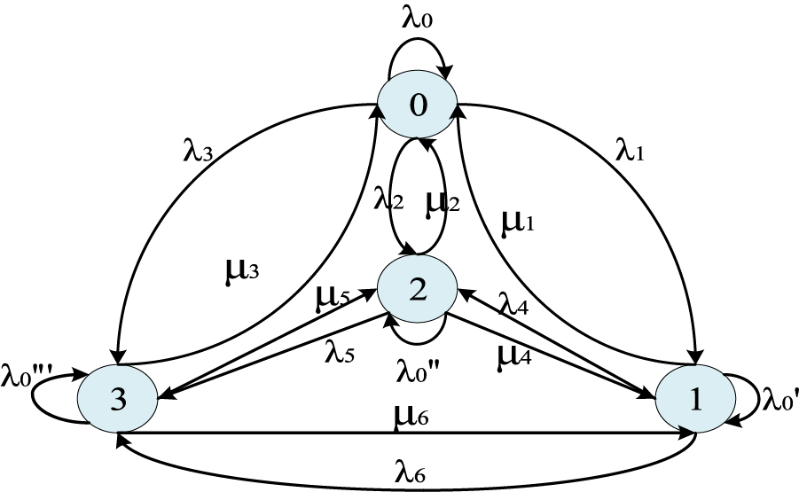
Figure 3: Diagram of Markov Chain to predict next state

States 1, 2, 3, and 4 in Fig. 3 represent four states of intra-group collision and idle, intra-group collision but not idle, no collision within the group but idle, no collision or idle within the group. The specific determination method is shown in the algorithm principle. λi,λ0n,μi represents the transition probability between states.

4.1.4 WOA Optimizes the C-Q Relationship

The Whale Optimization Algorithm (WOA) is inspired by the bubble-web feeding behavior of humpback whales in nature, it has three main stages: search for food, shrink surround, and spiral update position. In the Slot Prediction Q (SPQ) algorithm, the Vogt-II prediction algorithm is used only when the initial read or the system efficiency is continuously low, which effectively increases the lower limit of throughput. To further increase the upper limit of the SPQ algorithm, it is necessary to adjust the C-Q relationship. In the Q algorithm, step C has a linear relationship with the Q value, that is C=0.4×(1−Q15)+0.1. In this paper, WOA is used to search the target prey, that is the optimal C-Q relationship which can faster the speed of Q value adjusting. Specifically, it is to find a better C-Q relationship in advance in the simulation stage and write it to the RFID system in the form of list values, to speed up the process of adjusting Q values with C values.

4.2 Principle of SPQ Algorithm

Based on Q algorithm, the Slot Prediction Q (SPQ) algorithm introduces slot grouping and Vogt-II Prediction ideas. Based on the manually set Q_int, the SPQ algorithm predicts better Q_int through the recognition of the first frame, avoiding the situation that the initial Q value is too big to the actual tag number. In addition, because the Q algorithm only adjusts the frame length according to the current slot recognition situation, too many collision slots or idle slots will be generated, so the efficiency determination is set in the recognition process, and when the throughput rate continues to be low, the Vogt-II algorithm is used to accurately locate the appropriate frame length.

By comparing Eqs. (2)–(4), when frame length N is larger, the probability ratio of slot idle, read, and collision can be obtained by the formula which is shown in Eq. (7):

p0:pi=1e:1−2e≈1.4:1(7)

According to the idea of Framed Slotted ALOHA (FSA) algorithm, when the frame length is equal to the number of tags to be identified, the system has a maximum throughput of 36.8%, which is shown in Eq. (8):

p1:p0+p1+pi=0.368:1(8)

By combining Eqs. (7) and (8), the slot recognition expectation can be obtained by the formula which is shown in Eq. (9):

p0:p1:pi≈3.68:3.68:2.63(9)

Therefore, when the slot idle rate is greater than 0.4 or the slot collision rate is greater than 0.3, the gap between the number of tags to be read and the Q value is too large, and the Vogt-II prediction algorithm needs to be invoked to adjust the frame length.

The prediction of Vogt-II requires the recognition of a certain number of slots, so each slot grouping is required. In the general grouping idea, the efficiency of the algorithm decreases linearly with the increase of the number of slots in the group, but too small many slots will affect the prediction accuracy, so the corresponding number of slots is set into a group according to the Q value. At the same time, to avoid the influence of too small some tags, the prediction algorithm is not used when Q is less than 4, and the specific x-Q situation is analyzed by the Markov model.

In the grouping model, under the premise of p0>0.4||pi>0.3, the situation p0>0.4 within the group is intra-group idle and pi>0.3 is intra-group collision. Given that the number of tags to be identified is in the range of [64, 500] and the initial Q value is 4, the probability relationship of each state transition is obtained after repeated tests under different x. Take x = 0.6 Q as an example, and the data are shown in Table 1.

Substituting the state transition matrix is shown in Eq. (10):

A=[aij]N×N=[0.170.230.260.340.130.240.240.390.140.230.220.410.090.230.210.47](10)

The initial state of the model here refers to when the number of identified slots is greater than the number of packet slots, and the corresponding intra-group idle rate and collision rate of the first slot group meet, and in repeated tests the average value is shown in Eq. (11):

ζ(1)=[0.280.330.350.06](11)

Through the state transition matrix and the initial state, the next slot group state using the Vogt-II algorithm can be predicted by the formula which is shown in Eq. (12):

ζ(t)=ζ(t−1)×A(12)

The results of each prediction are averaged and compared, and after adjusting the frame length by Vogt-II is obtained in the case of x = 0.6Q that the expected value of the state matrix is shown in Eq. (13):

ζx=0.6Q=[0.110.230.240.42](13)

Change the pre-condition x-Q relationship, repeat the above steps, and the results are shown in Table 2.

The better expected value can be obtained when x = 0.4Q, which can be adjusted to the appropriate Q value by smaller slot number. For the case where the number of packet slots is large but the expected value is small, it is speculated that there is more than Vogt-II algorithm in the whole process of adjusting frame length, and the use of Q algorithm below the critical rate makes the overall optimization process of the system show an upward trend, so when p0>0.4||pi>0.3 is often the nearest slot throughput is low, and too many slots cannot achieve the ideal prediction effect.

The number of tags to be identified in Table 2 is only less than 500. To adapt to the actual unknown number of tags, different optimal x-Q relationships are obtained by changing the range of tag numbers. When the Q value is too large, the fixed slot number should be selected considering the time cost, and the results are shown in Table 3.

For cases where p0>0.4||pi>0.3 or Q values are not met, it is also expected to maximize the efficiency of the RFID system, so the optimal C-Q relationship is obtained by intelligent search through the Whale Optimization Algorithm (WOA).

In WOA, each whale records a C-Q function, and the individual fitness is represented by the throughput rate, which is the simulation result of the anti-collision algorithm. The process of whale hunting is shown in Fig. 4, since the target prey, namely the optimal solution, is unknown, the optimal individual of the population is selected as the temporary target, and a new population is initialized around the individual and presents an enveloping structure. There are two dynamic coefficients U and V in the iteration process. The expression is shown in Eq. (14):

U=2×u×rand−uV=|2×rand×X∗(t)−X(t)|(14)

where u decreases from 2 to 0 in the iteration process, so that the population gradually shrinks to surround the target, X represents the position of the current whale individual, X* represents the position of the optimal individual of the current population, then the position of the next iteration is expressed by the formula which is shown in Eq. (15):

X(t+1)=X∗(t)−U×V(15)

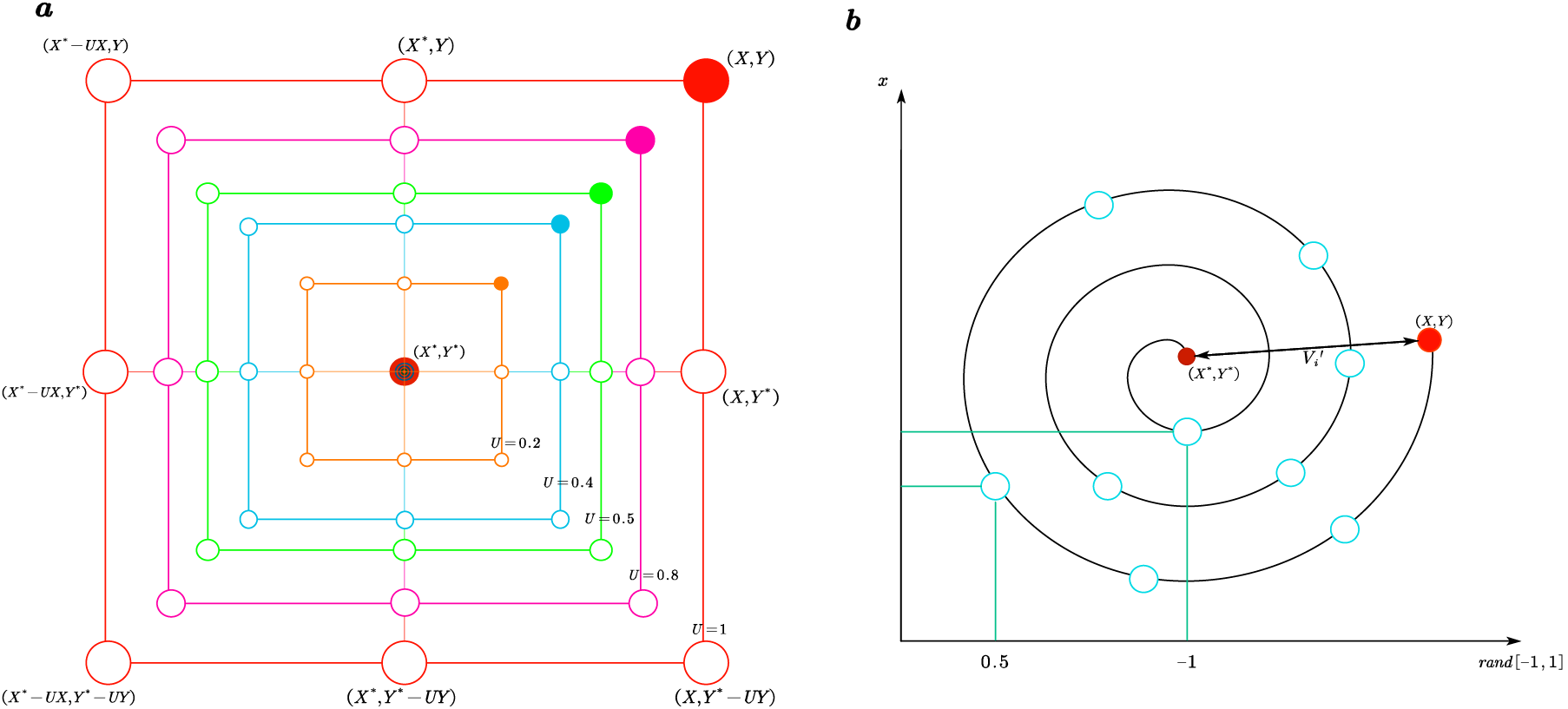
Figure 4: Diagram of Whale Optimization Algorithm simulated whale hunt

To fit a better value, the single linear relationship is abandoned, and the interval values of step C are directly set to the position of individual whales, which has evolved into a multi-dimensional variable optimization problem. To further simulate the shrinking encircling and spiraling trend of whales, the difference between target and individual is defined by the formula which is shown in Eq. (16):

V∗=|X∗(t)−X(t)|(16)

Add the constant coefficient b so that the iteration expression is shown in Eq. (17):

X(t+1)={X∗(t)−U×V,if rand <0.5V∗×eb⋅rand(−1,1)×cos⁡[2π⋅rand(−1,1)]+X∗(t),other(17)

The simulation parameters are as follows: variable dimension: 2, which are C and Q; Number of individuals: considering the overall reduction of error and time cost, the simulation is set to 100 (At first, the population number was set to 30, and the performance was average. Set to 150 and found that the performance becomes worse; Finally, the compromise is set to 100. The performance is better); Number of iterations: considering the reduction of error and time cost comprehensively, the simulation is set to 200; Upper and lower limits: the upper and lower limits of C are 0.1–0.5, and the upper and lower limits of Q are 0–15; Objective function: system efficiency. To avoid falling into the local optimal solution, the whale will also randomly search for the target. When U≥1 is set, the whale will stay away from the target and try to explore a better individual. The iterative results are shown in Fig. 5.

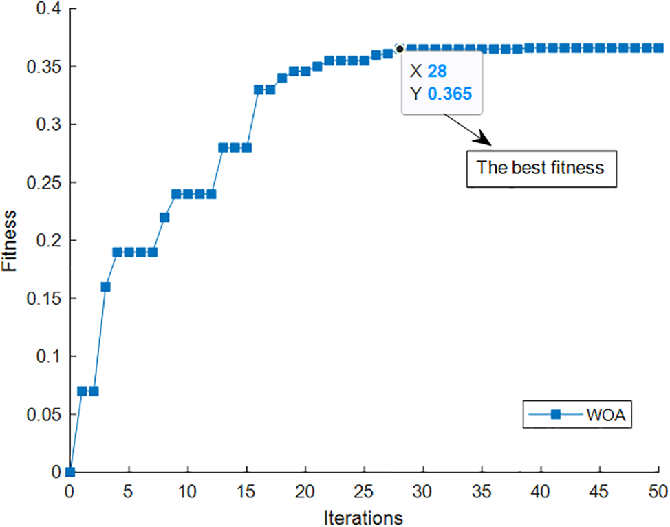
Figure 5: Iteration graph of Whale Optimization Algorithm in finding better C-Q relationship

The optimal C-Q relationship is obtained through searching, and the results are shown in Table 4.

4.3 Flow of SPQ Algorithm

The flow chart of the Slot Prediction Q (SPQ) algorithm is shown in Fig. 6, and its description is as follows:

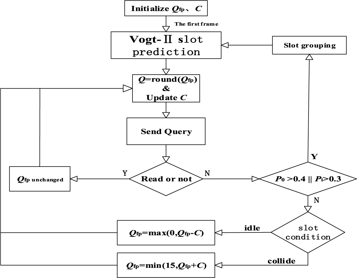
Figure 6: Flowchart of SPQ algorithm

step 1: The reader sets the initial Q_int, usually 4, sends the Query command and the tag to be read generates a random number at [0, 2Q− 1] and counts it to the slot counter.

step 2: If the Q value does not change during the reading process, the slot counter of the tag to be read decreases by 1, and the reader only reads the tag whose slot counter is 0. The reading cases are divided into idle slot c0, read slot c1 and collision slot ci.

step 3: Set the frame length N = 2Q according to Q_int, take the reading situation of one frame for Vogt-II grouping prediction, get the estimated number of tags to be read n, and carry out a new round of inventory according to the new Q value.

step 4: Slot idle rate p0 and slot collision rate pi are monitored in real-time. When the number of packet slots corresponding to the Q value is above, the expected idle rate and collision rate are compared. If the latter is above, Vogt-II prediction is performed according to the reading situation of the last x slots, and a new estimated tag number and Q value are obtained.

step 5: When p0 and pi are within the expected value, real-time detection of each slot reading situation. If it is read smoothly, the Q value remains unchanged, and the next slot of the frame continues. If the slot is idle or collides, the reader sends the “QueryAdjust” command to adjust the Q value, and the cycle repeats.

step 6: When the Q value changes at any time during the read, the reader immediately ends the current frame and sends a Query command to refresh the slot counter of the tag to be read based on the new Q value.

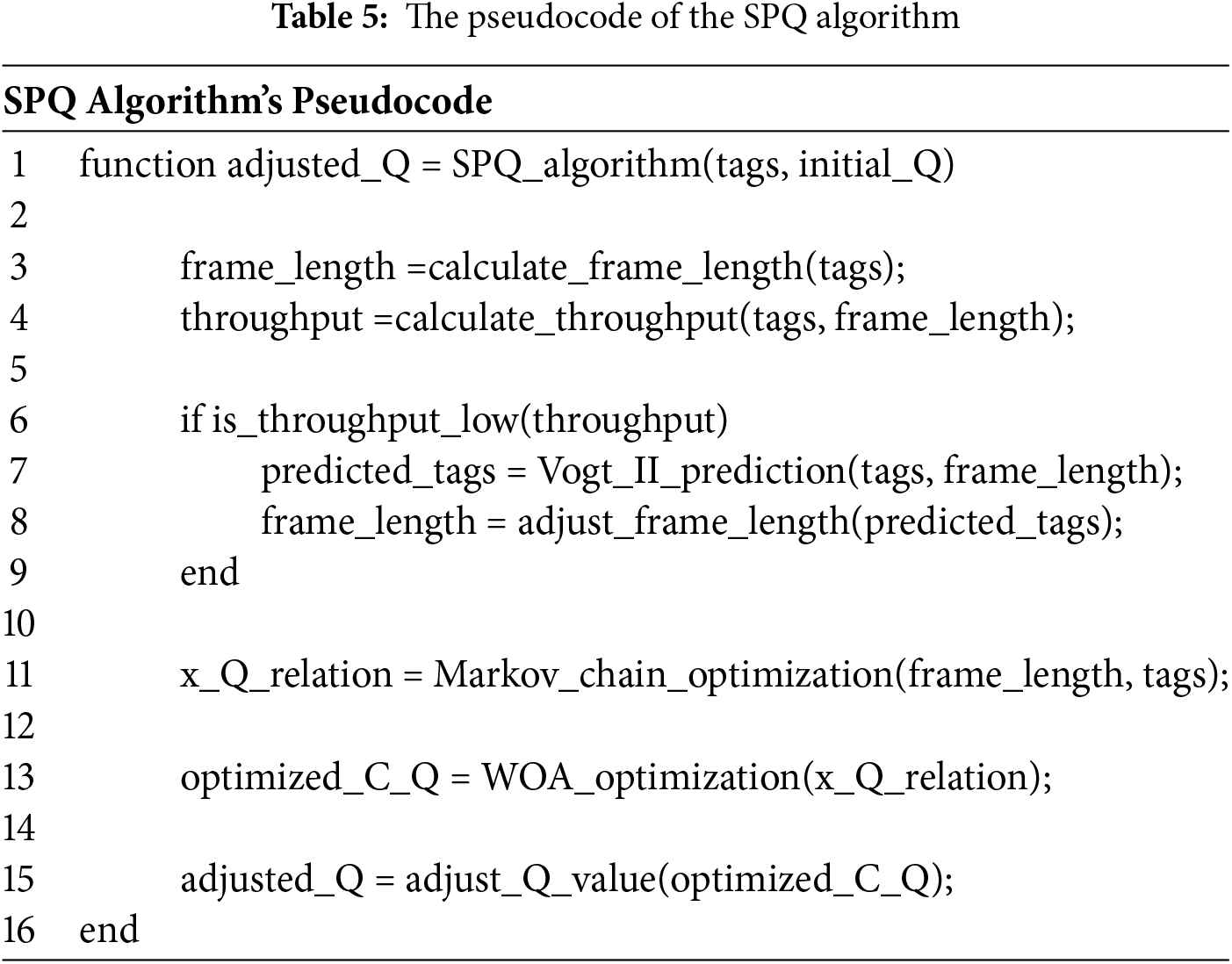
The pseudocode of the SPQ algorithm is shown in Table 5.

5  Simulation and Result Analysis

This paper simulates and analyzes the system performance by comparing the simulation results of traditional Q, Threshold Grouping Dynamic Q (TGDQ), FastQ, Subset Enhanced Performance-Q (SUBEP-Q), and the Slot Prediction Q (SPQ) algorithm proposed in this paper. Three indicators will be used for identification speed, system efficiency, and time efficiency.

The experimental simulation environment of this study is shown in Table 6.

According to the Electronic Product Code Global Class1 Generation2 (EPC Global C1 G2) standard, simulation parameters are shown in Table 7.

It takes time to define three kinds of slot recognition. Ts, Ti, and Tc respectively represent the time spent on successful recognition, slot-free, and slot collision. As shown in Fig. 7, their expression is shown in Eq. (18):

Ts=TEPC+2(T1+T2)+TRN16=1375.00μsTi=T1+T3=112.50μsTc=T1+T2+TRN16=337.50μs(18)

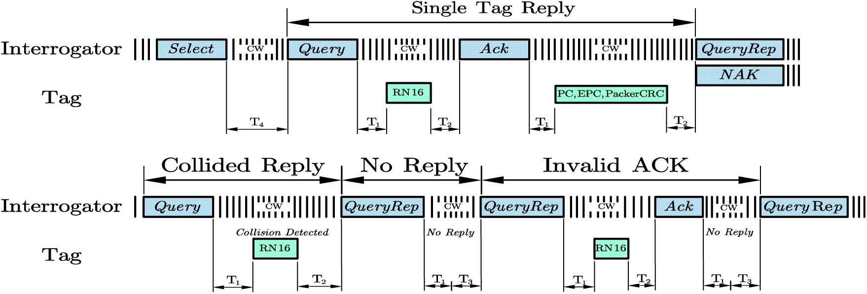
Figure 7: Diagram of electronic product code global class1 generation2 standard

Identification speed is an important indicator in the practical application of RFID system, in fact, many engineering projects to ensure the real-time system, the identification speed has certain requirements. Using the ratio of throughput to time at a given time, the identification speed is defined as Eq. (19):

SP=NsNsTs+NiTi+NcTc+TQuery(19)

Fig. 8 takes Q algorithm as the qualified line and simulates the recognition speed of each algorithm. As can be seen from the figure, the average recognition speed of Q algorithm is 403 n/s, while the average recognition speed of the SPQ algorithm reaches 432 n/s, which is 7.20% higher than Q algorithm. Obviously, by introducing slot group prediction mechanism and a better C-Q relationship, the recognition speed of SPQ algorithm has been significantly improved.

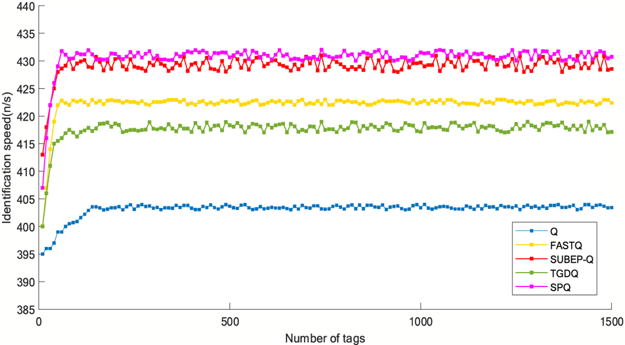
Figure 8: Simulation of identification speed

System efficiency is the core performance indicator of RFID systems, which is defined as Eq. (20):

S=TagsNumSlotNum=NsNs+Nc+Ni(20)

In the simulation, the inventory is finished only when all tags are read. Therefore, TagsNum is the same as the total number of s successfully identified on the inventory, and SlotNum is the total number of slots consumed on the inventory.

Fig. 9 compares system efficiency of Q, FastQ, TGDQ, SUBEP-Q and SPQ algorithms. Compared with the traditional dynamic frame slot algorithm, the biggest feature of the Q algorithm is that the system efficiency can reach about 32.5% at any number of tags. The SPQ algorithm optimizes the step parameters of Q algorithm by slot adjustment mechanism and uses slot grouping to predict the critical idle rate and critical collision rate, which makes up for the shortcoming of slow frame length adjustment of the traditional Q algorithm. Compared with the traditional Q value algorithm, the average system efficiency of SPQ algorithm is 36.1%, and the performance is improved by 11.08%.

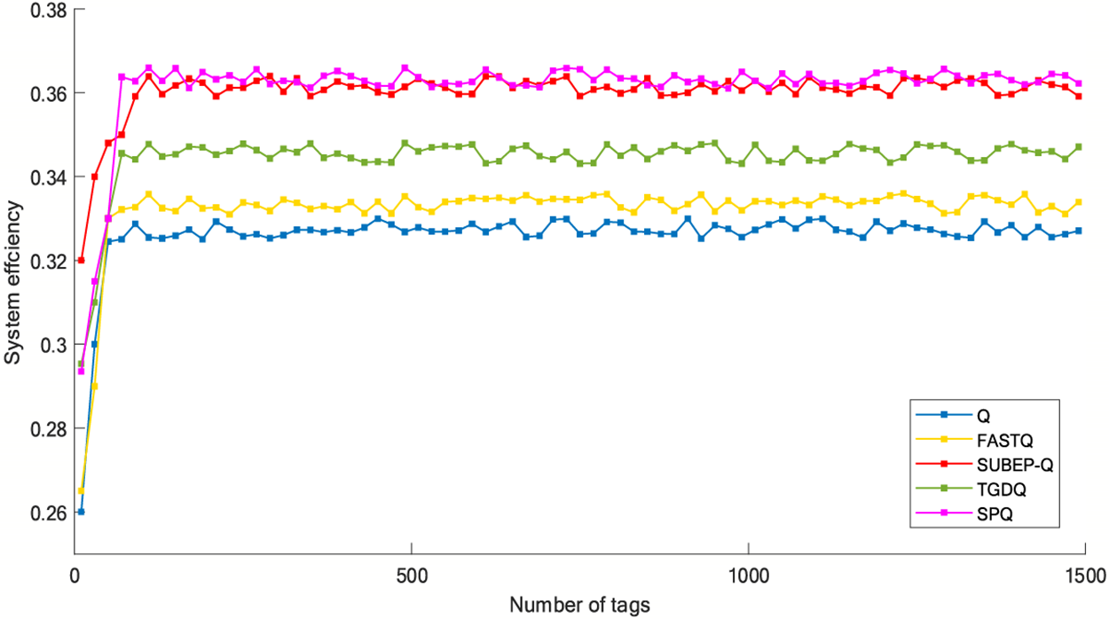
Figure 9: Simulation of system efficiency

In practical applications, in addition to improving the system throughput as much as possible, it is also necessary to consider the time efficiency, if you want to improve the time efficiency, the focus is on the efficiency and frequency of the anti-collision algorithm adjustment. Time efficiency is defined as Eq. (21):

O=NsTsNcTc+NsTs+NiTi(21)

Fig. 10 Simulated Q, FastQ, TGDQ, SUBEP-Q and SPQ algorithms. Compared with the same number of tags, the time efficiency of SPQ and SUBBEP-Q is similar, but slightly lower than that of FastQ, because the optimal ratio of collision slot to idle slot in FastQ changes dynamically. In order to improve the recognition speed, SPQ sets a fixed ratio, and adds the slot group prediction mechanism, which has a certain impact on the time efficiency. However, compared with Q algorithm, there is still a large improvement, so the cost is acceptable. The simulation results show that the average time efficiency of the SPQ algorithm is 5.69% higher than that of the Q algorithm when the number of 0–1500 tags to be identified is not considered.

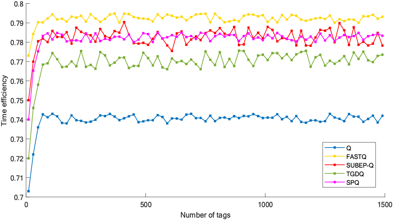
Figure 10: Simulation of time efficiency

6  Conclusion

This paper analyzes the development logic of ALOHA randomness algorithms and proposes the SPQ algorithm, which enhances the traditional Q algorithm by introducing key innovations such as a slot grouping mechanism, optimized adjustment steps, and improved C-Q relationships derived from the WOA. The SPQ algorithm retains the adaptive frame length adjustment feature of the Q algorithm while addressing its limitations, such as slow adjustment when the gap between frame length and tag number is too large. By leveraging a Markov model to determine the optimal x-Q relationship and using the WOA for refining the C-Q relationship, the SPQ algorithm achieves superior performance.

Simulation results confirm the effectiveness of the SPQ algorithm. It improves recognition speed, with an average speed of 432 n/s, 7.20% higher than the 403 n/s of the Q algorithm. System efficiency, a core performance metric of RFID systems, is enhanced to an average of 36.1%, representing an 11.08% improvement over the Q algorithm’s 32.5%. Although its time efficiency is slightly lower than that of FastQ due to a fixed slot ratio, the SPQ algorithm still achieves a 5.69% improvement compared to the Q algorithm. These improvements demonstrate the SPQ algorithm’s ability to achieve a balance between recognition speed, system efficiency, and time efficiency.

By exploiting slot grouping and real-time detection of idle and collision rates, the SPQ algorithm stabilizes system efficiency at a high level while enabling faster and more accurate frame length adjustments. These advantages position it as a practical and effective solution for RFID systems requiring real-time performance. Future research will focus on optimizing critical efficiency values, dynamically adjusting the ratio of collision to idle slots, and exploring other meta-heuristic algorithms to further enhance the algorithm’s performance.

Acknowledgement: The authors would like to thank the support by National Key Research and Development Program of China and National Natural Science Foundation of China.

Funding Statement: The study is supported by National Key Research and Development Program of China (2022YFB4703102) and National Natural Science Foundation of China (62273105).

Author Contributions: Jiacheng Luo completed the simulation experiment and wrote the paper. Jiahao Wen conceived the algorithm improvement direction and experimental scheme. Jian Yang gave guidance and revised the paper. All authors reviewed the results and approved the final version of the manuscript.

Availability of Data and Materials: The data used to support the findings of this study are available from the corresponding author upon request.

Ethics Approval: Not applicable.

Conflicts of Interest: The authors declare no conflicts of interest to report regarding the present study.

References

1. Suresh S, Chakaravarthi G. RFID technology and its diverse applications: a brief exposition with a proposed Machine Learning approach. Measurement. 2022;195(10):111197. doi:10.1016/j.measurement.2022.111197. [Google Scholar] [CrossRef]

2. Tan AT, Zainol Z. Flowgraph model for anti-collision authentication process in RFID system. Measurement. 2018;127:571–6. doi:10.1016/j.measurement.2018.05.077. [Google Scholar] [CrossRef]

3. Subrahmannian A, Behera SK. Chipless RFID: a unique technology for mankind. IEEE J Radio Freq Identif. 2022;6(6):151–63. doi:10.1109/JRFID.2022.3146902. [Google Scholar] [CrossRef]

4. Erman F, Koziel S, Leifsson L. Broadband/dual-band metal-mountable UHF RFID tag antennas: a systematic review, taxonomy analysis, standards of seamless RFID system operation, supporting IoT implementations, recommendations, and future directions. IEEE Internet Things J. 2023;10(16):14780–97. doi:10.1109/JIOT.2023.3289198. [Google Scholar] [CrossRef]

5. Chen Y, Su J, Yi W. An efficient and easy-to-implement tag identification algorithm for UHF RFID systems. IEEE Commun Lett. 2017;21(7):1509–12. doi:10.1109/LCOMM.2017.2649490. [Google Scholar] [CrossRef]

6. Unhelkar B, Joshi S, Sharma M, Prakash S, Mani AK, Prasad M. Enhancing supply chain performance using RFID technology and decision support systems in the Industry 4.0—a systematic literature review. Int J Inf Manag Data Insights. 2022;2(2):100084. doi:10.1016/j.jjimei.2022.100084. [Google Scholar] [CrossRef]

7. Chen WT. A feasible and easy-to-implement anticollision algorithm for the EPCglobal UHF class-1 generation-2 RFID protocol. IEEE Trans Automat Sci Eng. 2014;11(2):485–91. doi:10.1109/TASE.2013.2257756. [Google Scholar] [CrossRef]

8. Zhang R, Wang X, Chen J, Chen Y. Research on dynamic Q-value anti-collision algorithm based on tag grouping. In: IEEE 4th International Conference on Civil Aviation Safety and Information Technology (ICCASIT); 2022 Oct 12–14; Dali, China. p. 159–63. [Google Scholar]

9. Teng J, Xuan X, Bai Y. A fast Q algorithm based on EPC generation-2 RFID protocol. In: 2010 6th International Conference on Wireless Communications Networking and Mobile Computing (WiCOM); 2010 Sep 23–25; Chengdu, China. p. 1–4. [Google Scholar]

10. Zhang G, Tao S, Xiao W, Cai Q, Gao W, Jia J, et al. A fast and universal RFID tag anti-collision algorithm for the Internet of Things. IEEE Access. 2019;7:92365–77. doi:10.1109/ACCESS.2019.2927620. [Google Scholar] [CrossRef]

11. Yan J, Ye R, Zhong H, Jiang X. Twice labels number estimation algorithm based on gaussian fitting and chebyshev inequality. J Electron Inf Technol. 2021;43:1893. doi:10.11999/JEIT200209. [Google Scholar] [CrossRef]

12. Bonuccelli MA, Lonetti F, Martelli F. Instant collision resolution for tag identification in RFID networks. Ad Hoc Netw. 2007;5(8):1220–32. doi:10.1016/j.adhoc.2007.02.016. [Google Scholar] [CrossRef]

13. Cui Z, Lars Kirkby J, Nguyen D. A general framework for time-changed Markov processes and applications. Eur J Oper Res. 2019;273(2):785–800. doi:10.1016/j.ejor.2018.08.033. [Google Scholar] [CrossRef]

14. Arismendi R, Barros A, Grall A. Piecewise deterministic Markov process for condition-based maintenance models—application to critical infrastructures with discrete-state deterioration. Reliab Eng Syst Saf. 2021;212(4):107540. doi:10.1016/j.ress.2021.107540. [Google Scholar] [CrossRef]

15. Jamal W, Das S, Oprescu IA, Maharatna K. Prediction of synchrostate transitions in EEG signals using Markov chain models. IEEE Signal Process Lett. 2015;22(2):149–52. doi:10.1109/LSP.2014.2352251. [Google Scholar] [CrossRef]

16. Mirjalili S, Lewis A. The whale optimization algorithm. Adv Eng Softw. 2016;95(12):51–67. doi:10.1016/j.advengsoft.2016.01.008. [Google Scholar] [CrossRef]

17. Nadimi-Shahraki MH, Zamani H, Asghari Varzaneh Z, Mirjalili S. A systematic review of the whale optimization algorithm: theoretical foundation, improvements, and hybridizations. Arch Comput Methods Eng. 2023;37(30):4113–59. doi:10.1007/s11831-023-09928-7. [Google Scholar] [PubMed] [CrossRef]

18. Mohammed HM, Umar SU, Rashid TA. A systematic and meta-analysis survey of whale optimization algorithm. Comput Intell Neurosci. 2019;2019(1):8718571. doi:10.1155/2019/8718571. [Google Scholar] [PubMed] [CrossRef]

19. Kaur G, Arora S. Chaotic whale optimization algorithm. J Comput Des Eng. 2018;5(3):275–84. doi:10.1016/j.jcde.2017.12.006. [Google Scholar] [CrossRef]