Large-Scale 3D Thermal Transfer Analysis with 1D Model of Piped Cooling Water

1  Introduction

Recently, an integrated coal gasification combined cycle (IGCC) plant [1], which is a next-generation thermal power generation plant with low emissions of air pollutants and carbon dioxide, has been under development. In this plant, pulverized coal is fired under high temperatures and high pressure in a gasifier reactor, and then coal gas and slag are extracted. The temperature and pressure reach 2000°C and 3 MPa [2]. Because operation under high temperatures affects the structural integrity of the reactor vessel, cooling pipes are embedded in the reactor vessel to control the temperature with water. To accelerate the development of the reactor, numerical simulations are useful. Some researchers have worked on numerical simulations of combustion processes in a coal gasifier reactor [3,4]. However, although coupled analysis considering combustion, water cooling, heat conduction in the vessel and structural deformation of the vessel is important for evaluation of the structural integrity of the reactor vessel in actual operation conditions, such coupled analysis has not been reported so far. It is so challenging because tons of degrees of freedom (DOFs) are required to model the reactor which has complicated geometry and to capture various phenomena. Although our final goal is to develop the coupled analysis that can be performed within practical computational time, the present study focused on numerical simulations for heat conduction phenomena of the reactor vessel with water cooling pipes.

For solving coupled problems between conduction phenomena in solids and convection phenomena in fluids, a conjugated heat transfer approach is often used. For example, it was applied to the cooling of rocket engines [5] and the cooling of hot stamping tools [6]. However, this approach is computationally expensive. Because we put emphasis on computational efficiency, we assumed fluid velocity in pipes to be given and constant, and the temperature of the fluid to be governed by the one-dimensional (1D) convection-diffusion equation. The similar simplification is seen in studies on the cooling of concrete [7–9]. In these studies, concrete was discretized by three-dimensional (3D) solid elements, while cooling water was discretized by line elements. However, the line elements must be located at an edge or run across a solid concrete element, which engenders inconvenience in model preprocessing. Moreover, these studies did not consider the exact shape of concrete because pipes were represented by lines. Due to these drawbacks, the applications of the analysis systems proposed in these studies were limited to simple-shaped structures that were not modeled by many DOFs.

In the cooling problem of our interest, the size of the pipes is not enough small to be neglected. Unlike the above studies [7–9], we used a geometrically exact model. Because of complex geometry, the modeling of the reactor vessel requires a huge number of DOFs. The novelty of the present study was to develop an efficient numerical analysis system that can handle large-scale cooling analysis of complicated-shaped structures. To achieve high efficiency, the proposed analysis system had three features: (1) the meshes for cooled objects and cooling water can be prepared individually, (2) the system is parallelized, and (3) the fast evaluation of the heat exchange is implemented.

One of the methods for solving coupled problems is partitioning [10,11], where a coupled analysis system is constructed from multiple sub-analysis systems, which are executed sequentially. In partitioned methods, the use of existing sub-solvers is allowed. Therefore, it is easy to develop parallelized systems. Additionally, the use of non-matching meshes enables us to prepare independent meshes for sub-analysis systems [12]. In the present study, by employing a partitioned approach with non-matching meshes and choosing parallelized existing solvers as sub-solvers, the features (1) and (2) were realized. The use of non-matching meshes makes it time-consuming to calculate the amount of data exchanged between sub-solvers. As a countermeasure, we proposed a Dirac delta function-based interpolation. Then, the feature (3) was realized.

The rest of this paper is organized as follows. In Section 2, we explain how to model a cooled object, cooling water in pipes, and heat exchange between them. In Section 3, the coupled analysis for the present heat conduction and cooling problems is described. The discretizations for the cooled object and that of the cooling water in pipes are given. Then, we explain the data exchange method between the two models for the calculation of the source terms involved with heat exchange. At the end of this section, we provide the details of the proposed coupled analysis system. In the proposed system, for the heat transfer analysis of the cooled object, we employed an opensource large-scale parallel solver, ADVENTURE_Thermal [13–15], and for the convective heat transfer analysis of the cooling water in pipes, a 1D discontinuous Galerkin (DG) method-based solver of a convection-diffusion equation was developed and used. Because the required time step size for the analysis of the cooling water in pipes is much smaller than that for heat conduction phenomena in the cooled object, we introduced a subcycling technique [12]. In Section 4, the proposed analysis system is verified by solving a problem of water cooling of concrete. In Section 5, we simulate the water cooling phenomena of a laboratory-scale coal gasifier reactor to demonstrate that the proposed analysis system can handle a large-scale and practical problem on a supercomputer. Finally, concluding remarks are given in Section 6.

2  Modeling

Fig. 1 shows the schematic view of a problem with water cooling in a pipe. Ωt and Ωw are the domains of the cooled object and the cooling water in the pipe, respectively. Γtw is the interface between the cooled object and the cooling water. In the present study, the thickness of the pipe is assumed to be zero. The centerline of a pipe, denoted by Λc, is defined using the arc-length parameter l as

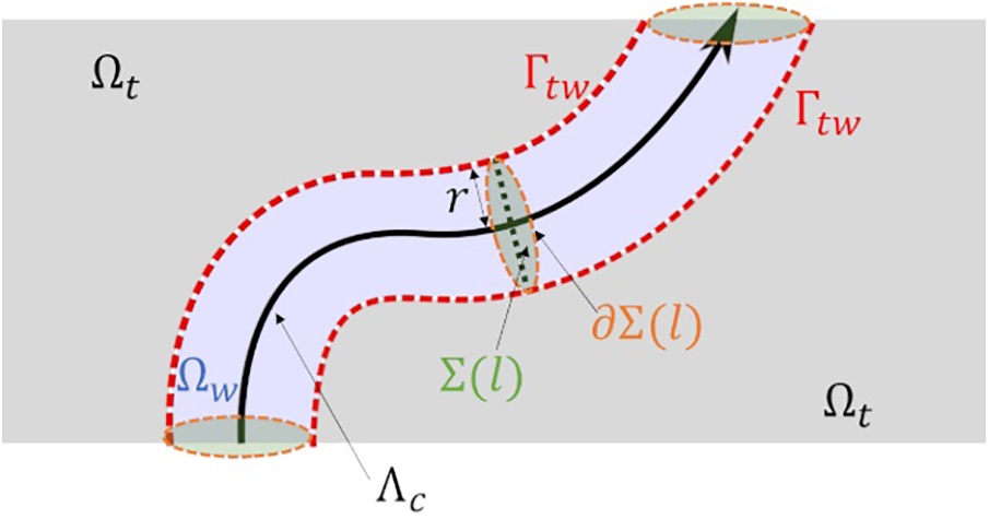
Figure 1: Schematic view of the water cooling problem

Λc={x=(x,y,z)∣x=xp(l),y=yp(l),z=zp(l),0≤l≤Lp}(1)

where Lp is the length of the centerline. The surface of the pipe, which corresponds to Γtw, is defined as

Γtw={x=(x,y,z)∣(x−xp(l))⋅vp(l)=0,‖x−xp(l)‖=r,0≤l≤Lp}(2)

where r is the radius of the pipe, and xp(l) and vp(l) are defined as

xp(l)=(xp(l),yp(l),zp(l)),vp(l)=(∂xp(l)∂l,∂yp(l)∂l,∂zp(l)∂l)(3)

Note that ‖vp‖=1 holds because l is the arc-length parameter. In Fig. 1, Σ(l) is the cross section of the pipe, which can be described as

Σ(l)={x=(x,y,z)∣(x−xp(l))⋅vp(l)=0,‖x−xp(l)‖≤r}(4)

The boundary of Σ(l) can be written as ∂Σ(l)=Γtw∩Σ(l).

In this section, heat transfer models for the cooled object and the cooling water are explained. Then, the modeling of heat exchange between the two models is explained.

2.1 Cooled Object

The temperature field of the cooled object, denoted by Tt, is governed by the following unsteady heat equations:

ρtct∂Tt∂t=∇⋅(κt∇Tt)(5)

where ρt, ct, and κt are the mass density, the specific heat, and the thermal conductivity of the cooled object, respectively. In the present study, we assume that no heat source exists and thermal conduction is isotropic. On the interface Γtw, the following boundary condition is prescribed:

κt∇Tt⋅n=h(6)

where n is the unit outward normal vector and h is the heat flux from the cooling water. The determination of h is explained in Section 2.3.

2.2 Cooling Water in Pipe

The temperature field of the cooling water in each pipe is governed by a 1D convection-diffusion equation. The derivation of the equation is explained here. We have some assumptions for the cooling water. First, on the cross section Σ(l), the velocity vector of the water is Vwvp(l), where Vw is the magnitude of the velocity vector, and it is constant. Second, on the cross section Σ(l), the temperature of the water, denoted by Tw1D(l), is uniform. Third, the mass density of the water ρw and the specific heat of the water cw are both uniform.

We consider the energy balance in a small volume ΔΩw(l′), which is the volume surrounded by Γtw, Σ(l′), and Σ(l′+Δl). The law of conservation of energy can be written as

Est=Eindiff−Eoutdiff+Einadv−Eoutadv+Esur(7)

where Est is the power generated in ΔΩw(l′):

Est=ρwcw∫ΔΩw(l′)∂Tw1D(l,t)∂tdΩ=ρwcwA‖vp‖∫l′l′+Δl∂Tw1D(l,t)∂tdl(8)

where A=πr2 is the area of the cross section. Eindiff and Eoutdiff are respectively the inflow and the outflow of the power due to diffusion:

Eindiff=−κwA∂Tw1D(l′,t)∂l(9)

Eoutdiff=−κwA∂Tw1D(l′+Δl,t)∂l(10)

where κw is the thermal conductivity of the cooling water. Einadv and Eoutadv are the respective inflow and outflow of power due to the advection:

Einadv=ρwcwAVwTw1D(l′,t)(11)

Eoutadv=ρwcwAVwTw1D(l′+Δl,t)(12)

Esur is the power associated with the heat exchange:

Esur=−∫ΔΓtwh dΓ=−‖vp‖∫l′l′+Δl(∫∂Σ(l)h ds)dl(13)

where ΔΓtw is the interface between the cooled object and the cooling water in ΔΩw(l′). From Eqs. (7)–(13), the following equation is obtained under the condition Δl→0:

∂Tw1D(l′,t)∂t=−Vw∂Tw1D(l′,t)∂l+D∂∂l(∂Tw1D(l′,t)∂l)−1ρwcwA∫∂Σ(l′)h ds(14)

where we use ‖vp‖=1, and D is D=κwρwcw.

2.3 Heat Exchange

The heat flux on Γtw is based on Newton’s law of cooling. At an arbitrary point on Γtw, the coordinate of which is xa, the heat flux is calculated as

h(xa)=−H(Tt(xa)−Tw1D(la))(15)

where H is the heat transfer coefficient and la is the coordinate of a point on Λc closest to xa, as shown in Fig. 2. This orthographic projection is described using an operator ℳ:

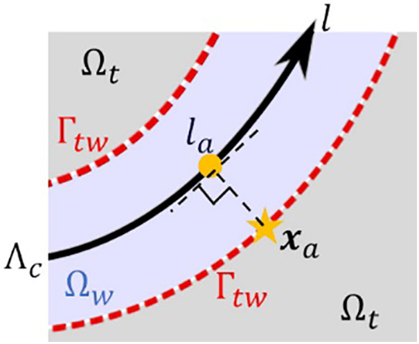
Figure 2: Position where water temperature is used for Newton’s law of cooling

la=ℳ(xa)(16)

3  Proposed Analysis Method

3.1 Discretization for Cooled Object

In the heat transfer analysis of the cooled object, Eqs. (5) and (6) are solved. The following weak form is considered:

ρtct∫Ωtψt∂Tt∂tdΩ+κt∫Ωt∂ψt∂x∂Tt∂x+∂ψt∂y∂Tt∂y+∂ψt∂z∂Tt∂zdΩ=∫Γtwψth dΓ(17)

where ψt(x) is the weight function. For the spatial discretization, we employ the FE method with linear 4-node tetrahedral elements. Here, we assume h, defined in Eq. (15), can be approximated by the FE interpolation:

h(x)≈∑I∈PNI(x)h(xI)=−H∑I∈PNI(x)(Tt(xI)−Tw1D(ℳ(xI))),x∈Γtw(18)

where NI is the shape function associated with a node I, xI is the coordinate of node I, and 𝒫 is the set of nodes on the interface Γtw.

For the time integration scheme, the backward Euler method is employed. As explained in Section 3.4, the temperature of the cooling water in Eq. (18) is treated explicitly.

3.2 Discretization for Cooling Water

In the heat transfer analysis of the cooling water, the local DG method [16] is employed. The following two equations derived from Eq. (14) are considered:

∂Tw1D∂t=−∂∂l(F+Z)−S(19)

Z(l)=−D∂Tw1D(l)∂l(20)

where F is F(l)=VwTw1D(l) and S is S(l)=1ρwcwA∫∂Σ(l)h ds. The domain of the cooling water Λc is divided into NEw elements with NEw+1 points, the coordinates of which are represented by l1,l2,⋯,lNEw+1. The domain of the i-th element is denoted by Λci=(li,li+1). Multiplying Eqs. (19) and (20) by a weight function ψw, and integrating the result over an element Λci, we obtain:

∫Λciψw∂Tw1D∂tdl=∫Λci∂ψw∂l(F+Z)dl−[ψw(F+Z)]lili+1−∫ΛciψwSdl(21)

∫ΛciψwZdl=∫ΛciD∂ψw∂lTw1Ddl−[DψwTw1D]lili+1(22)

In the DG method, the boundary terms associated with F are approximated by a numerical flux. All other boundary terms (terms associated with Z and Tw1D) are approximated by averaging. For more details, see reference [17]. As a result, Eqs. (21) and (22) are rewritten as Eqs. (23) and (24), respectively:

∫Λciψw∂Tw1D∂tdl=∫Λci∂ψw∂l(F+Z)dl−ψw(li+1−)F(li+1−)+ψw(li+)F(li+)−ψw(li+1−)(Z(li+1+)+Z(li+1−)2)+ψw(li+)(Z(li+)+Z(li−)2)−∫ΛciψwSdl(23)

∫ΛciψwZdl=∫ΛciD∂ψw∂lTw1Ddl−Dψw(li+1−)(Tw1D(li+1+)+Tw1D(li+1−)2)+Dψw(li+)(Tw1D(li+)+Tw1D(li−)2)(24)

For an arbitrary function with an input l, denoted by α, α(l+) and α(l−) are defined as

α(l±)=lima→±0α(l+a)(25)

Each element has nl local nodes, and the shape functions for the element are the (nl−1)-th order Lagrange polynomials. In the present study, nl=3.

For the time integration scheme, the forward Euler method is employed. The procedures for solving Eqs. (23) and (24) are as follows. First, Z is updated by solving Eq. (24) under the explicit treatment of Tw1D. Second, Tw1D is computed by solving Eq. (23) using the updated Z and explicit treatment of F. Here, the last term on the right-hand side of Eq. (23) is explicitly treated. However, the discretization of the term is complicated. Therefore, we introduce an approximation, which is explained in Section 3.3.

3.3 Approximation of Source Term Involved with Heat Exchange

In Section 3.1, the discretized form of the source term involved with the heat exchange [∫ΓtwψthdΓ in Eq. (17)] is described as h3D. We here provide a simple procedure using h3D for the numerical integration of ∫ΛciψwSdl in Eq. (23). Let a function h~(x) be defined as

h~(x)=∑I∈PhI3Dδ(x−xI)(26)

where hI3D is the I-th component of h3D and δ(x) is the Dirac delta function. After h is replaced by h~, the discretized form of ∫ΛciψwSdl, denoted by h1D, is calculated as

h(i,I)1D=∫ΛciN(i,I)DGSdl≈1ρWcwA∫Λci∫∂Σ(l)N(i,I)DGh~ds dl=1ρWcwA∑J∈PN(i,I)DG(ℳ(xJ))hJ3D(27)

where h(i,I)1D is a component of h1D, N(i,I)DG is the shape function, and both are associated with the I-th local node in element i. This scheme needs no numerical quadrature. Therefore, under the condition that h3D is given, this scheme is simple and convenient.

3.4 Coupling Method between 3D Analysis for Cooled Object and 1D Analysis for Cooling Water

In the present study, cooling problems are considered as coupled problems between cooled objects and cooling water in pipes. For coupled analysis methods, we employ a partitioned method, which executes multiple sub-solvers sequentially. The advantage of the partitioned methods is that they allow the use of existing solvers, which makes it easy to develop parallel analysis systems by choosing parallel solvers as sub-solvers. Because a gasifier reactor has a complex geometry, a huge number of DOFs is needed for modeling, and parallel computing is imperative. It is thus reasonable to adopt a partitioned method.

For the 3D heat transfer FE analysis of the cooled object, we employed ADVENTURE_Thermal [13–15], which is a module in the ADVENTURE system [18]. ADVENTURE is an opensource general-purpose computational mechanics system based on the FE method. The system was designed with the ability to analyze a 3D FE model of arbitrary shape with 10 million to 1 billion DOFs. The hierarchical domain decomposition method [19] with a preconditioned iterative solver has been implemented in ADVENTURE_Thermal.

In contrast, for 1D analysis of cooling water, in-house code for a DG method was developed and used. Implicit time integration is employed for the 3D FE analysis. Conversely, explicit time integration is employed for the 1D DG analysis. Therefore, the time step size for 1D DG analysis has to be much smaller than that for the 3D FE analysis. Hence, we employed a subcycling technique.

The flowchart of the proposed analysis system is shown in Fig. 3. Here, the variables with the superscript (n) represent those at the n-th time step, and the variables with the subscript (k) represent those at the k-th subcycle. N is the number of subcycles. In procedure I, the temperature of the cooling water is treated explicitly. In procedure II, h3D is computed using Tt(n+1) and Tw1D(n). In procedure IV, Tw1D(k)(n+1) is used for Tw1D in Eq. (24). In procedure V, Z(k+1)(n+1) and F(k)(n+1)=VwTw1D(k)(n+1) are used for Z and F in Eq. (23), respectively.

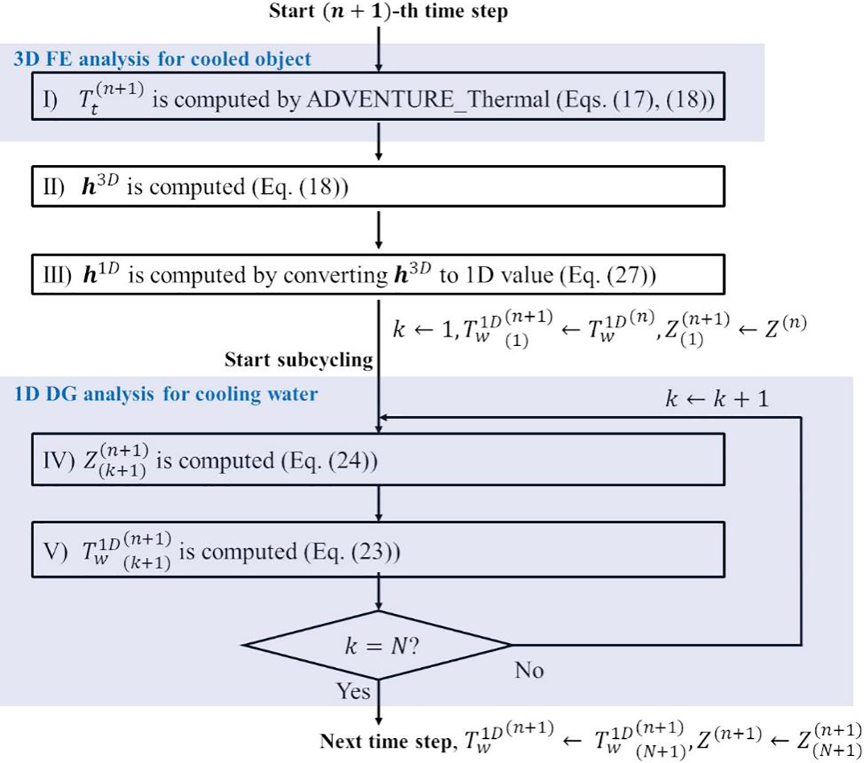
Figure 3: Flowchart of the proposed analysis system

Regarding the implementation, the functions corresponding to II) to V) in Fig. 3 were incorporated into ADVENTURE_Thermal.

4  Verification

4.1 Problem Setting

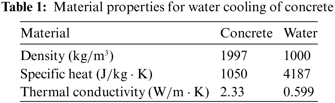
For verification, the water cooling of concrete was considered [20]. The geometry is shown in Fig. 4. The radius of the concrete was 0.845 m. The height was 200 m. The concrete included a straight pipe with a radius of 0.014 m. The material properties are listed in Table 1. The water flowed in the positive z direction with water velocity Vw=0.406m/s. The heat transfer coefficient was 200W/m2⋅K, which was determined based on the study by Liu et al. [8]. The initial temperature of the concrete was 293.15 K. The initial temperature of the water and the temperature of the water at the inlet were both 277.15 K. An adiabatic boundary condition was imposed on all surfaces of the concrete except the interface Γtw.

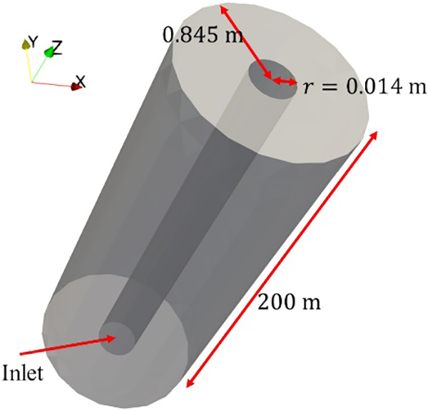
Figure 4: Geometry of concrete cooling verification problem

For the discretization of the concrete, the number of nodes was 1,527,987, and the number of elements was 7,487,914. For the discretization of the water, the number of nodes was 1500 and the number of elements was 500. The time step size of the 3D heat transfer analysis by ADVENTURE_Thermal was 3600 s. The number of subcycles was 360,000.

For parallel computing of ADVENTURE_Thermal, the domain was decomposed into 12 parts, each of which had 100 subdomains. For the domain decomposition, ADVENTURE_Metis [21], which was developed based on the graph partitioning module PARMETIS [22], was employed. The workstation used for the analysis had a 2.7 GHz Intel Xeon Gold 6150 processor and 392 GB of DDR4 memory.

4.2 Results

The distribution of the temperature of the cooling water is shown in Fig. 5. “Position” in x-axis label means the distance from the inlet. The cooling water warmed as it flowed in the positive z direction because it received heat from the concrete. The distribution of the temperature in the concrete is shown in Fig. 6. For visualization, z coordinates are scaled to be 1%. The cross section through the center of the pipe is depicted. Because the heat exchange occurred at the interface (Γtw), the concrete near the pipe was cooled faster than far from the pipe. Because heat was not generated in the concrete and 4°C water flowed in constantly through the pipe, the water and concrete temperature keep dropping and approached 4°C everywhere.

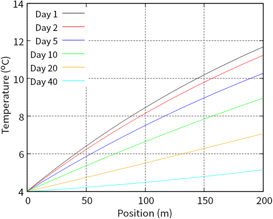
Figure 5: Distribution of temperature in concrete cooling water on different days

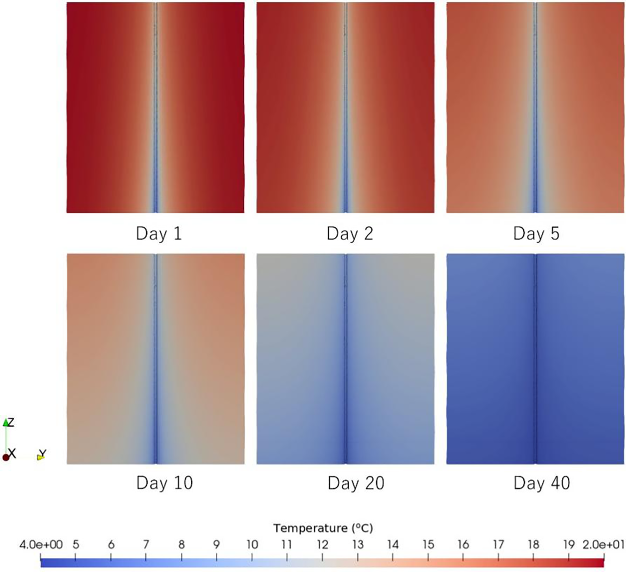
Figure 6: Distribution of temperature in concrete on different days

Zhu provided the analytical solution of the cooling problem as

Tave=4.0+16.0e−1.609(0.03319τ)1.0282(28)

where Tave is the average temperature of the concrete and τ is the time in days. Fig. 7 shows the transition of the average temperature of the concrete. We can see good agreement between the numerical and analytical solutions.

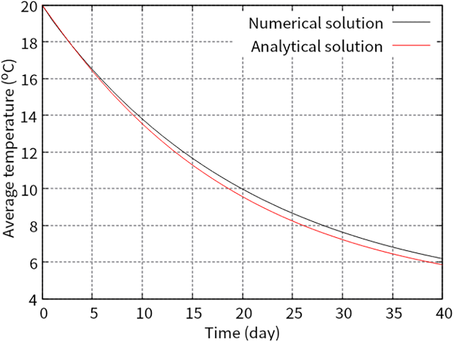
Figure 7: Time history of average temperature in concrete

The computational time of the 3D FE analysis per time step was 61.9 s. That of the 1D DG analysis for 360,000 subcycles was 232 s.

The results described in this section qualitatively and quantitatively verified the developed analysis system.

5  Analysis of Water Cooling for Coal Gasification Reactor

This section demonstrates that the proposed analysis system can handle very large-scale problems with complicated geometries and can be operated in a supercomputer environment.

5.1 Problem Setting

The Central Research Institute of the Electric Power Industry (CRIEPI) has been developing a laboratory-scale coal gasifier reactor [23], which is the target of the computation in this section. The geometry of the reactor with cooling pipes is shown in Fig. 8.

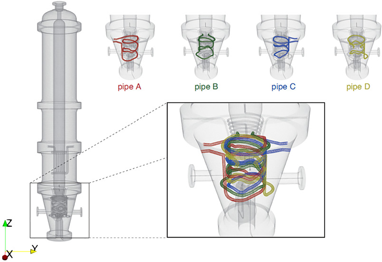
Figure 8: Gasifier reactor with four cooling pipes

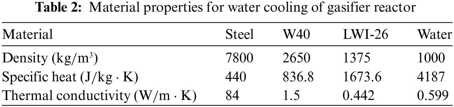
The cross section of the reactor is shown in Fig. 9. The reactor is a hollow structure, and as it operates, pulverized coal is turned to gas in the reactor interior. Because the target of the present study is a coupling analysis between the thermal transfer phenomenon acting on the reactor and the convection-diffusion phenomenon acting on the cooling water in the pipes, the combustion phenomenon in the hollow chamber [4] is outside the scope of the present study. The reactor is composed of three parts: an outer shell made of steel, heat-resistant material made of W40, and heat-resistant material made of LWI-26. The number of pipes is four, and they are labeled as Pipes A, B, C, and D in Fig. 8. The radius of each pipe is 0.0136 m. The lengths of Pipes A, B, C, and D are 4.549, 4.559, 4.556, and 4.587 m, respectively. The material properties are listed in Table 2.

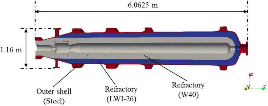
Figure 9: Cross section of the gasifier reactor

The water velocity Vw was 1.703 m/s. The initial temperature of the reactor was 1273.15 K. The initial temperature of the water and the temperature of the water at the inlet were 298.15 K. An adiabatic boundary condition was imposed on all surfaces of the reactor except the interfaces Γtw.

The heat transfer coefficient can be written as

H=κwNu2r(29)

where Nu is the Nusselt number. To determine Nu, we employ the Dittus-Boelter equation:

Nu=0.023Re0.8Pr0.4(30)

In the present study, the Reynolds number Re and Prandtl number Pr were 4.632×104 and 6.990, respectively. As a result, H was determined to be 5957W/m2⋅K.

For the discretization of the reactor, the number of nodes was 25,510,852, and the number of elements was 155,999,061. For pipe A, the water was discretized by 516 nodes and 172 elements. For pipes B, C, and D, the water was discretized by 522 nodes and 174 elements. The time step size for ADVENTURE_Thermal was 0.1 s. The number of subcycles was 1000.

For parallel computing of ADVENTURE_Thermal, the domain was decomposed into 480 parts, each of which had 400 subdomains. For this computation, we used 40 nodes with 12 cores of Fugaku [24], which is a recently built manycore-based parallel system developed as a Japanese national flagship supercomputer in the FLAGSHIP 2020 Project, and was ranked No. 1 in the Top 500 after performing 442 Petaflops in June 2020.

5.2 Results

Figs. 10 and 11 show the distribution of the temperature on the cross section through the YZ plane at different times. Fig. 10 visualizes the whole structure, while Fig. 11 shows the local one around the cooling pipes. The figures show that the temperature of the reactor decreased, especially around the pipes.

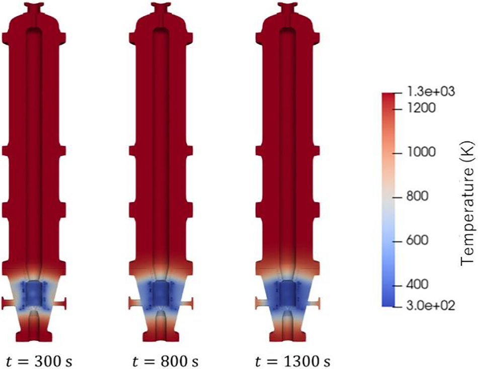
Figure 10: Distribution of temperature in the whole reactor at different times

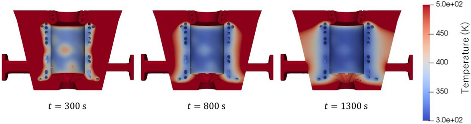
Figure 11: Distribution of temperature around cooling pipes at different times

Fig. 12 shows the distribution of the temperature in the cooling water of Pipes A, B, C, and D. The four subfigures in Fig. 12 are similar. At the beginning of the cooling, there was big difference between the temperature of the cooling water and that of the pipe surfaces. Therefore, a large amount of heat was exchanged, and the water temperature increased suddenly. As the cooling proceeded, the temperature of the pipe surfaces decreased. Therefore, the temperature difference gradually became smaller and the amount of exchanged heat decreased. Then, the water temperature decreased as time passed.

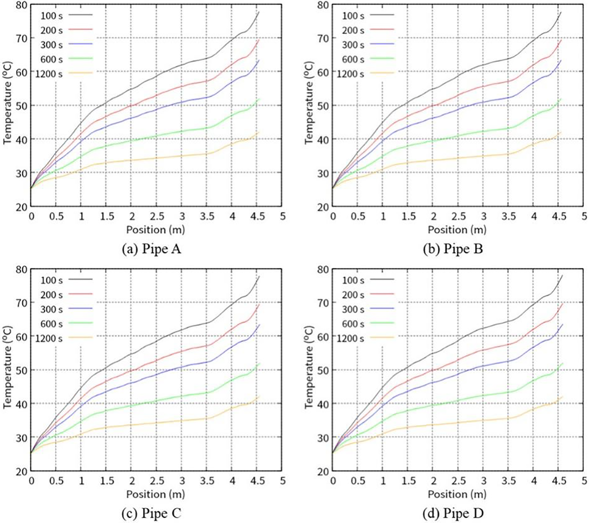
Figure 12: Distribution of temperature in cooling water at different times: (a) Pipe A, (b) Pipe B, (c) Pipe C, and (d) Pipe D

The computational time of the 3D FE analysis per time step was 8.16 s. That of the 1D DG analysis for 1000 subcycles was 7.61 s.

This section described how our proposed analysis was applied to the cooling problem for a gasification reactor. The results we obtained were reasonable and confirmed that our analysis system can handle large-scale problems with complex geometry.

6  Conclusions

The present study developed a new coupled analysis system for problems on water cooling in pipes. The system employs a partitioned approach with non-matching meshes and a subcycling technique. For the heat transfer analysis of a cooled object, we employed an opensource 3D FEM large-scale parallel solver, ADVENTURE Thermal. For the convective heat transfer analysis of the cooling water in pipes, a 1D DG method-based solver of a convection-diffusion equation was developed and used. To make it easy to compute heat exchange, we proposed a Dirac delta function-based interpolation. The system was verified by solving a problem with water cooling of concrete. Then, we confirmed the system can handle a large-scale problem with complicated geometry and can be operated in a supercomputer environment.

Our final goal is to develop a coupled analysis considering combustion, water cooling, heat conduction in the vessel and structural deformation of the vessel for evaluation of the structural integrity of the reactor vessel in actual operation conditions. In the subsequent study, we plan to integrate a combustion analysis solver with the proposed analysis system.

Acknowledgement: The present study was supported in part by the Program for Promoting Research on the Supercomputer Fugaku (Digital Twins of Real World’s Clean Energy Systems with Integrated Utilization of Super-Simulation and AI) and JSPS KAKENHI, and used computational resources of the supercomputer Fugaku provided by the RIKEN Center for Computational Science. The authors thank Drs. Akio Makino and Shiro Kajitani for providing technical advice and information and data on CRIEPI’s laboratory-scale coal gasification plant.

Funding Statement: The present study was supported by the Program for Promoting Research on the Supercomputer Fugaku (Grant Number JPMXP1020200303) and JSPS KAKENHI (Grant Number JP22K17902).

Author Contributions: The authors confirm contribution to the paper as follows: study conception and design: S. Kaneko, N. Mitsume; data collection: S. Kaneko; analysis and interpretation of results: S. Kaneko, S. Yoshimura; draft manuscript preparation: S. Kaneko. All authors reviewed the results and approved the final version of the manuscript.

Availability of Data and Materials: The data that support the findings of this study are available from the corresponding author, upon reasonable request.

Conflicts of Interest: The authors declare that they have no conflicts of interest to report regarding the present study.

References

1. Batorshin, V. A., Suchkov, S. I., Tugov, A. N. (2023). Integrated gasification combined cycle (IGCC) units: History, state-of-the art, development prospects. Thermal Engineering, 70, 418–429. [Google Scholar]

2. Kenji, T., Ahn, S., Watanabe, H. (2017). Numerical study of effects of operation condition for Oxygen blown coal gasifier in oxy-fuel IGCC. Proceedings of the International Conference on Power Engineering, Charlotte, USA. [Google Scholar]

3. Abani, A., Ghoniem, A. F. (2013). Large eddy simulations of coal gasification in an entrained flow gasifier. Fuel, 104(1), 664–680. [Google Scholar]

4. Watanabe, H., Kurose, R. (2020). Modeling and simulation of coal gasification on an entrained flow coal gasifier. Advanced Powder Technology, 31(7), 2733–2741. [Google Scholar]

5. Nasuti, F., Torricelli, A., Pirozzoli, S. (2021). Conjugate heat transfer analysis of rectangular cooling channels using modeled and direct numerical simulation of turbulence. International Journal of Heat and Mass Transfer, 181, 121849. [Google Scholar]

6. Hu, P., He, B., Ying, L. (2016). Numerical investigation on cooling performance of hot stamping tool with various channel designs. Applied Thermal Engineering, 96, 338–351. [Google Scholar]

7. Kim, J. K., Kim, K. H., Yang, J. K. (2001). Thermal analysis of hydration heat in concrete structures with pipe-cooling system. Computers & Structures, 79, 163–171. [Google Scholar]

8. Liu, X., Zhang, C., Chang, X., Zhou, W., Cheng, Y. et al. (2015). Precise simulation analysis of the thermal field in mass concrete with a pipe water cooling system. Applied Thermal Engineering, 78, 449–459. [Google Scholar]

9. Chao, Y., Li, T., Qi, H., Liu, X., Cheng, J. (2022). A partitioned iterative method based on externally embedded cooling water pipe elements for mass concrete temperature field. International Journal for Numeric and Analytical Methods in Geomechanics, 46, 2337–2355. [Google Scholar]

10. Felippa, C. A., Park, K. C., Farhat, C. (2001). Partitioned analysis of coupled mechanical systems. Computer Methods in Applied Mechanics and Engineering, 190, 3247–3270. [Google Scholar]

11. Kaneko, S., Hong, G., Mitsume, N., Yamada, T., Yoshimura, S. (2018). Numerical study of active control by piezoelectric materials for fluid-structure interaction problems. Journal of Sound and Vibration, 24, 23–35. [Google Scholar]

12. Farhat, C., Lesoinne, M., Maman, N. (1995). Mixed explicit/implicit time integration of coupled aeroelastic problems: Three-field formulation, geometric conservation and distributed solution. International Journal for Numerical Methods in Fluids, 21, 807–835. [Google Scholar]

13. Mukaddes, A., Ogino, M., Shioya, R. (2014). The study of thermal-solid coupling problems using open source CAE software. Procedia Engineering, 90, 147–153. [Google Scholar]

14. Mukaddes, A., Ogino, M., Shioya, R., Kanayama, H. (2017). Treatment of block-based sparse matrices in domain decomposition method. International Journal of System Modeling and Simulation, 2, 1–6. [Google Scholar]

15. Mukaddes, A., Shioya, R., Ogino, M., Roy, D., Jaher, R. (2021). Finite element-based analysis of bio-heat transfer in human skin burns and afterwards. International Journal of Computational Methods, 18(3), 2041010. [Google Scholar]

16. Cockburn, B., Shu, C. (1998). The local discontinuous Galerkin method for time dependent convection-diffusion systems. SIAM Journal on Numerical Analysis, 35, 2440–2463. [Google Scholar]

17. Dawson, C., Kubatko, E., Westerink, J., Trahan, C., Mirabito, C. et al. (2011). Discontinuous galerkin methods for modeling hurricane storm surge. Advances in Water Resources, 34, 1165–1176. [Google Scholar]

18. Yoshimura, S., Shioya, R., Noguchi, H., Miyamura, T. (2002). Advanced general-purpose computational mechanics system for large-scale analysis and design. Journal of Computational and Applied Mathematics, 149, 279–296. [Google Scholar]

19. Yagawa, G., Shioya, R. (1993). Parallel finite elements on a massively parallel computer with domain decomposition. Computing Systems in Engineering, 4, 495–503. [Google Scholar]

20. Zhu, B. (1999). Effect of cooling by water flowing in nonmetal pipes embedded in mass concrete. Journal of Construction Engineering and Management, 125(1), 61–68. [Google Scholar]

21. Murotani, K., Sugimoto, S., Kawai, H., Yoshimura, S. (2014). Hierarchical domain decomposition with parallel mesh refinement for billions-of-DOF scale finite element analyses. International Journal of Computational Methods, 11(4), 1350061. [Google Scholar]

22. Karypis, G., Schloegel, K., Kumar, V. (1997). PARMETIS: Parallel graph partitioning and sparse matrix ordering library. https://hdl.handle.net/11299/215345 (accessed on 04/01/2023). [Google Scholar]

23. Watanabe, H., Tanno, K., Umetsu, H., Umemoto, S. (2012). A numerical simulation on an O2-CO2 blown coal gasifier-Modeling of O2-CO2 blown coal gasification and evaluation of gasification characteristics. https://criepi.denken.or.jp/hokokusho/pb/reportDetail?reportNoUkCode=M11017 (accessed on 04/01/2023). [Google Scholar]

24. Sato, M., Ishikawa, Y., Tomita, H., Kodama, Y., Odajima, T. et al. (2020). Co-design for A64FX manycore processor and “Fugaku”. Proceedings of the International Conference for High Performance Computing, Networking, Storage and Analysis, pp. 1–16. Atlanta, GA, USA. [Google Scholar]