A Single-Ended Protection Principle for LCC-VSC-MTDC System with High Resistance Fault Tolerance

1  Introduction

In recent decades, high voltage direct current (HVDC) transmission technology based on line-commutated converter (LCC) converters has become the mainstream solution for DC lines. However, with the continuous construction of high-voltage DC lines, the problem of commutation failure caused by the centralized feeding of multiple DCs has become increasingly prominent, which seriously impacts the security and stability of the power grid. The currently emerging three-terminal hybrid DC transmission technology uses the LCC sending end to connect two modular multilevel converters (MMC) receiving ends. The advantage that the MMC receiving end does not have commutation failure has become a new method to solve the commutation failure problem of multi-circuit centralized DC feeding into the power grid [1–3]. Currently under construction, China’s Wudongde DC transmission project will become the world’s first three-terminal hybrid DC transmission project [4,5].

DC line protection is the first line of defense to ensure the safe and stable operation of DC lines. At present, the traveling wave protection principle of DC transmission lines includes two categories: Use time-domain information such as amplitude and differential and use frequency domain information such as frequency difference [6,7]. Time-domain mutation protection is mainly divided into two types: Epipolar and modulus [8,9]. However, when the transition resistance of the fault in the DC line area is large or the distance between the fault point and the protection installation is long, the mutation of the traveling wave will be greatly attenuated, causing the protection to refuse to operate [10].

Aiming at the insufficient sensitivity of the principle-based on abrupt changes in the time domain, scholars proposed a protection principle constructed by using the energy information in the frequency domain [11]. The method uses time-frequency analysis tools such as S-transform to extract energy and then uses the high-low frequency energy ratio as the protection criterion [12]. However, this protection principle is mainly applied to traditional DC and MMC DC grids and does not consider the characteristics of the three-terminal hybrid DC system. At present, there are few related studies on the three-terminal hybrid DC line protection. Reference [13] studied common main and backup protection action coordination. However, this reference is only an overview of existing protections and does not propose new protection schemes. Reference [14] proposed a fault area identification method for DC lines to realize fault area identification of each line in a DC system. However, this scheme relies on strong boundary elements and is less applicable. Reference [15] analyzed the waveform-related characteristics of electrical quantities in the time-domain, and used pattern recognition to distinguish fault types. The characteristic of relying on the same fault waveform makes it unsuitable for hybrid DC transmission systems. Reference [16] took the integral ratio of the traveling wave amplitude at both ends of the line as the judgment basis. Reference [17,18] proposed that the filtering characteristics of boundary elements in UHVDC transmission systems have a blocking effect on the high-frequency components generated by out-of-area faults. Reference [19] proposed an ultra-high-speed DC protection principle based on the traveling wave correlation coefficient. The existing LCC-VSC system has a diversity of boundary elements, and the above literature is difficult to apply to the topology of different boundary elements.

It can be, therefore, extrapolated from the above analysis that the principle of the Hybrid DC System system still faces problems such as the reliability of protection, the complexity of the implementation process, and the ability to resist transition resistance, and the speed of protection. Therefore, further in-depth research is still needed to propose a protection principle with selectivity, quickness, sensitivity, and reliability for DC lines. To ensure the reliable and safe operation of the LCC-VSC multi-terminal direct current (MTDC) system, a single-ended protection principle based on the traveling wave transmission coefficient is proposed. This paper’s main work and contributions are: 1) The simplified circuit and the first traveling wave of the LCC-VSC hybrid DC system are analyzed, respectively. 2) The calculation method of transmission coefficient is introduced, and a single-ended protection principle based on multi-frequency transmission coefficient is proposed. 3) Compared with existing solutions, the principle proposed in this paper has better resistance to high resistance (600 Ω) and noise interference (10 dB).

Section 2 analyzes the traveling wave process of the hybrid DC transmission system and derives its first traveling wave expression. The calculation method and fault characteristics of the multi-frequency transmission coefficient are analyzed in Section 3. Section 4 gives the flow and details of the proposed protection principle. Subsequently, the LCC-VSC-MTDC transmission system model verifies the correctness and superiority of the proposed principle, and conclusions are provided in Section 5.

2  Topology and Equivalent Circuit

In this section, the topology of the LCC-VSC-MTDC system is given first; then its equivalent circuit and the first traveling wave expressions are analyzed. Finally, using transmission coefficients to identify fault types is proposed.

2.1 Topology and Equivalent Circuits

This paper takes the LCC-MMC-MMC parallel three-terminal hybrid DC transmission system as the object to study, and its topology is shown in Fig. 1. The sending end of the system is the LCC converter station, and the two receiving ends are MMC converter stations. The DC line is divided into two sections, Line1 and Line2. Line1 is connected to one of the converter stations MMC1 through the DC busbar and then connected through Line2. The next receiving end converter station is MMC2. Each converter station is equipped with smoothing reactors, among which the LCC converter station is also equipped with a DC filter; the system adopts the double-pole plus neutral grounding method.

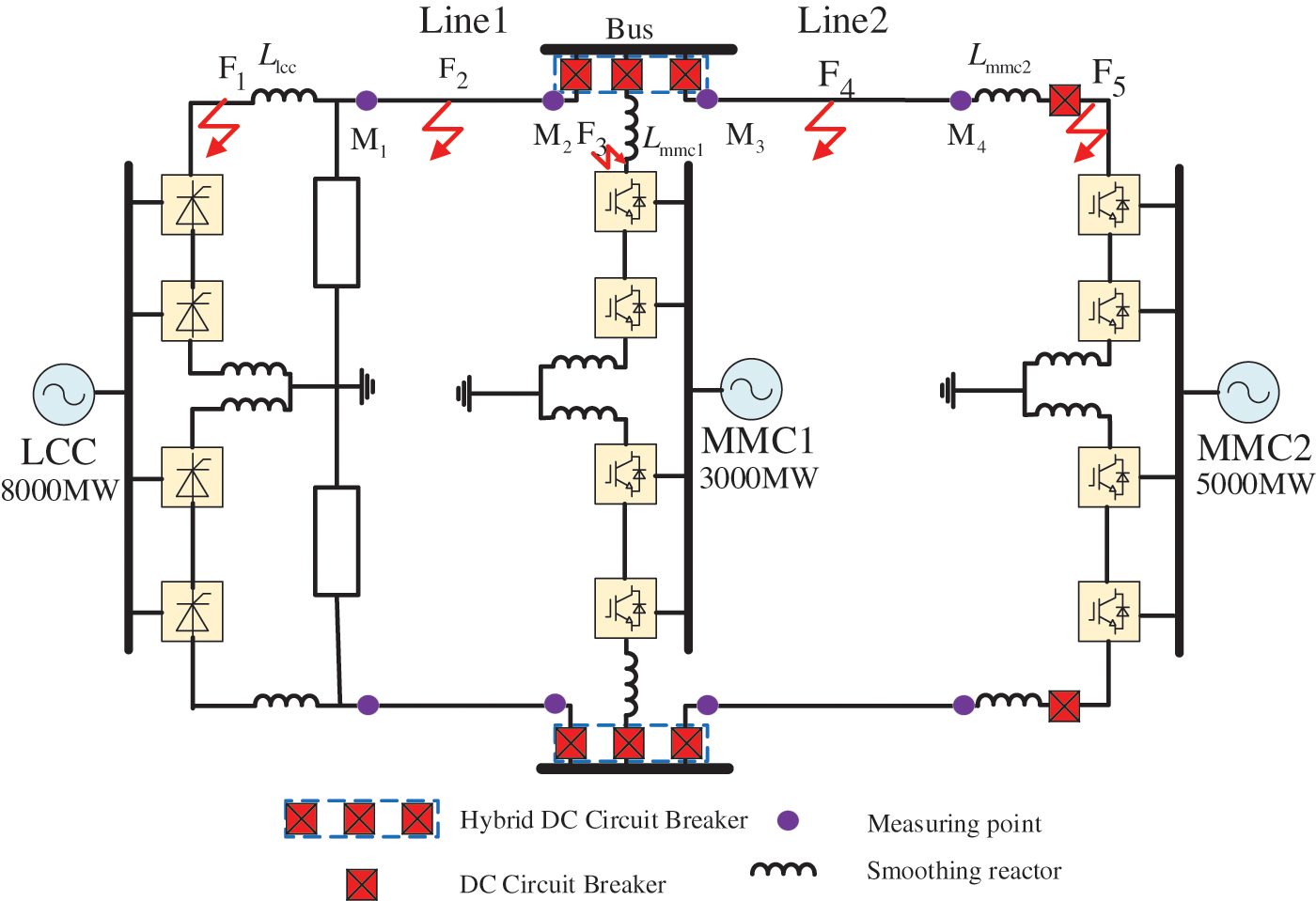
Figure 1: Topological structure of LCC-VSC-MTDC DC grid

According to Fig. 1, the equivalent circuit of LCC-VSC-MTDC is obtained as shown in Fig. 2. Llcc, Lmmc1 and Lmmc2 respectively represent the current-limiting reactors at the outlet of the three-terminal converter; ZC2 and ZC3 represent the wave impedance of the lines Line1 and Line2, respectively; Zmmc1 and Zmmc2 represent the equivalent impedance of the converters MMC1 and MMC2, including the equivalent inductance (Lcmmc1 and Lcmmc2), capacitance (Ccmmc1 and Ccmmc2) and resistance (Rcmmc1 and Rcmmc2); Zfliter represents the equivalent impedance of the DC filter, including equivalent inductance (L11/21 and L12/21), capacitance (C11/21 and C12/22).

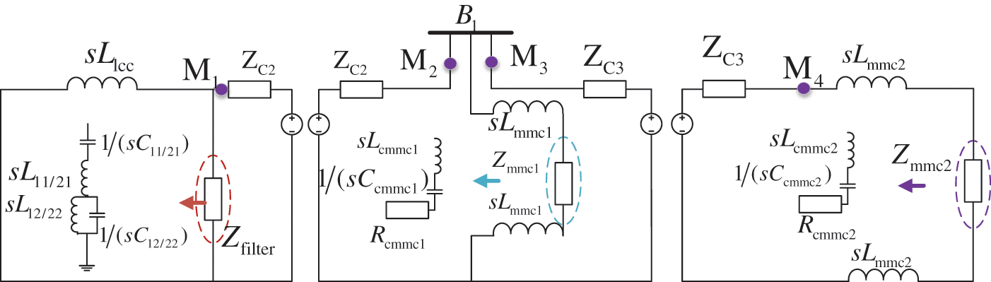
Figure 2: Topology and equivalent circuit of LCC-VSC-MTDC system

2.2 First Traveling Wave

Traditional headline expressions such as formula (1) are [20]:

I=e−γ(s)xIx(1)

where I represents the measuring point current, Ix represents the fault point current, γ(s) represents the propagation coefficient. When there is an external fault, the expressions of the first traveling wave of different fault circuits are quite different. Therefore, it is necessary to derive the first traveling wave expression for the LCC-VSC-MTDC system. Analyze the transmission process of the first traveling wave of Line1 and Line2 to obtain the equivalent circuit. It is worth noting that the first traveling wave process does not involve the catadioptric behavior of traveling waves.

(1)   Line1

The traveling wave fault circuit of Line1 is shown in Fig. 3. In Fig. 3, ZB and ZC1 represent the equivalent impedance of the busbar and the line, respectively. BAf1(s) represents the equivalent voltage source; Uf′(s) represents the fault excitation voltage source; U(x,s) and I(x,s) represent fault point traveling-wave; U(0,s) and I(0,s) respectively represent the traveling wave voltage and current at the measurement point.

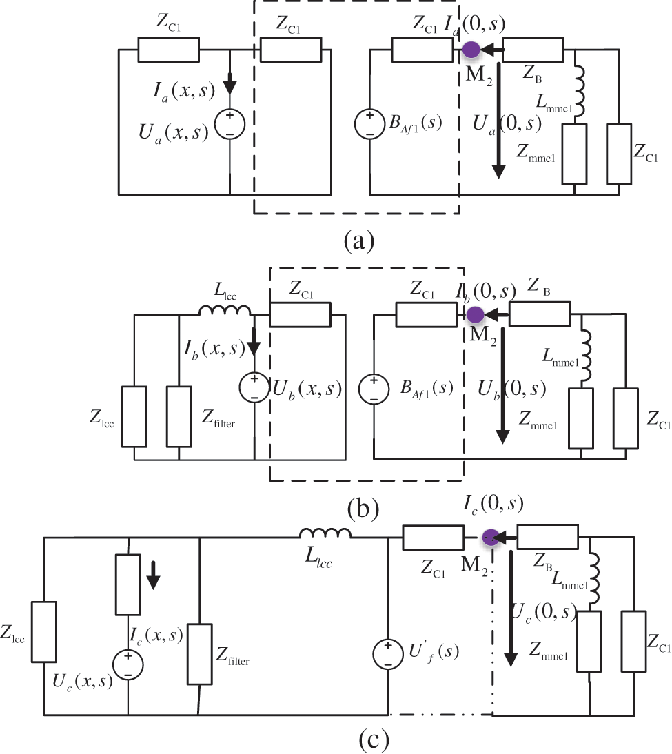
Figure 3: Internal and external fault equivalent circuit of Line1. (a) Midpoint internal fault, (b) End internal fault, (c) External fault

Fig. 3a represents the equivalent circuit of the internal midpoint faults. When the internal midpoint faults occur, the Line1 model splits into two parts when the internal midpoint faults occur. In the middle, a fault port circuit has been added to connect to the two-segment circuit model and the converter station. Figs. 3b and 3c represent the equivalent circuit of the internal terminal fault and external fault. Since there is no new fault port when the line end fails, the fault excitation voltage source will directly act on the equivalent circuit. In the event of an external fault, the additional fault voltage source is transmitted to the measurement point via the line boundary element. When comparing the equivalent circuit, however, it can be seen that the boundary element causes the difference in the first traveling wave of the fault. Therefore, the first traveling wave formula is:

{Internal midpoint fault{:}Ia(0,s)=e−(a(ω)+jβ(ω))x−Ua(x,s)(sLmmc1+Zmmc1)//ZC1+ZBInternal end fault{:}Ib(0,s)=e−(a(ω)+jβ(ω))x−Ub(x,s)ZB+(sLmmc1+Zmmc1)//(ZC1)External fault{:}Ic(0,s)=e−(a(ω)+jβ(ω))x−Uc(x,s)∙eβlccZB+(sLmmc1+Zmmc1)//(ZC1)(2)

where {α(ω)=12[raga−ω2laca+(ra2+ω2la2)(ga2+ω2ca2)]β(ω)=12[ω2laca−raga+(ra2+ω2la2)(ga2+ω2ca2)]; ra, ga, ca and la represent the resistance, conductance, capacitance, and inductance per unit length of the line, respectively; eβlcc represents the attenuation coefficient of the boundary element on the LCC side.

(2)   Line2

The analysis process of Line2 is the same as that of Line1. Its equivalent circuit is shown in Fig. 4. Different from Line1, the boundary elements of the MMC converter include bus bars and current limiting reactors. Therefore, the first traveling wave of Line2 is shown as follows:

{Internal midpoint fault{:}Id(0,s)=e−(a(ω)+jβ(ω))x−Ud(x,s)sLmmc2+Zmmc2Internal end fault{:}Ie(0,s)=e−(a(ω)+jβ(ω))x−Ue(x,s)sLmmc2+Zmmc2External fault{:}If(0,s)=e−(a(ω)+jβ(ω))x−Uc(x,s)∙eβBsLmmc2+Zmmc2(3)

where eβB represents the attenuation coefficient of the MMC boundary element.

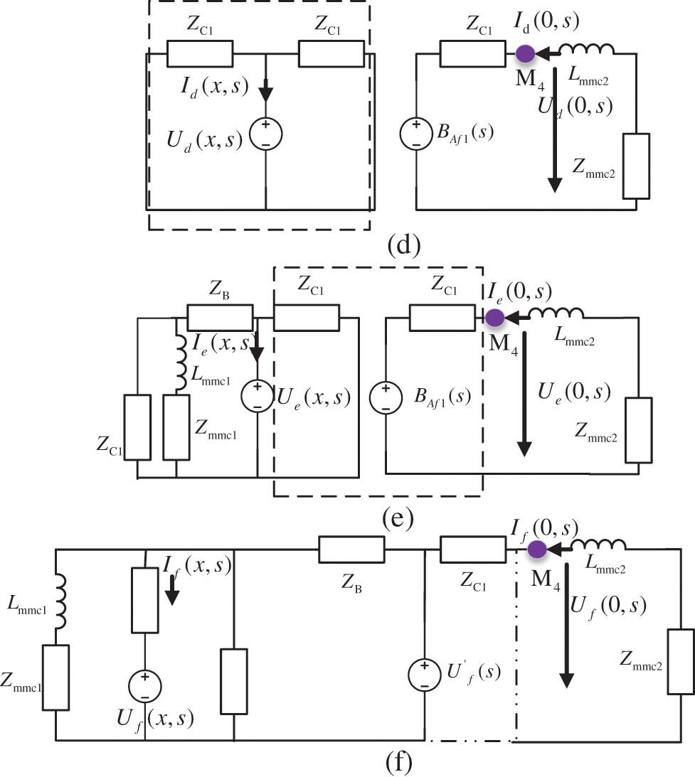
Figure 4: Internal and external fault equivalent circuit of Line2. (d) Midpoint internal fault, (e) End internal fault, (f) External fault

If the attenuation-related parameters in the expression are extracted, the eigenvalues that are not affected by the fault resistance can be constructed. Since line attenuation expressions are closely related to line parameters, boundary element attenuation coefficients are closely related to boundary element parameters. Such frequency-varying parameters make the expression difficult to analyze quantitatively. Therefore, this paper proposes a method of fitting transmission coefficients to construct fault identification criteria.

3  Multi-Frequency Transmission Coefficient

The analysis in Section 2 shows that the transmission coefficient in the first traveling wave expression can identify the fault type. This chapter first proposes a method for fitting the transfer coefficient. Then the attenuation characteristics of lines and boundary elements are analyzed, and the concept of multi-frequency transmission coefficient is proposed accordingly.

3.1 Fitted Transfer Coefficient

This section proposes to use the Gauss-Newton method to fit the attenuation part to obtain the fault coefficient. The expression of the first traveling wave is a nonlinear curve, which can be written as:

F(x)=∑i=1mfi2(x)(4)

The first-order Taylor expansion fi(x) is approximated by ϕi(x) to get:

ϕi(x)=∇fi(xk)Tx−[∇fi(xk)Txk−fi(xk)];i=1,2,⋯,m(5)

According to formulas (4) and (5), (6) can be obtained:

φ(x)=∑i=1mϕ2i(x)=(∇f1(xk)T⋮∇fm(xk)T)x+(∇f1(xk)T−f1(xk)⋮∇fm(xk)T−fm(xk))(∇f1(xk)T⋮∇fm(xk)T)x+(∇f1(xk)T−f1(xk)⋮∇fm(xk)T−fm(xk))(6)

Each time iterative calculation is performed, φ(x) is used to represent F(x). Given Ak, b and fk the expressions are:

Ak=(∇f1(xk)T⋮∇fm(xk)T),b=(∇f1(xk)T−f1(xk)⋮∇fm(xk)T−fm(xk))=Akxk−fk,fk=[f1(xk)⋮fm(xk)]

At this point, approximating φ(x)=∑i=1mϕ2i(x) and setting its derivative to 0.

{AkTAkx=AkT(Akxk−fk)x−xk=−(AkTAk)−1AkTfk(7)

where xk+1=x is the extreme point of a single iteration. It is composed of two parameters, the function value of fi(xk) and the value of the first-order partial derivative. Both parameters need to be updated on each iteration. Therefore, the calculation process of the transmission coefficient is as follows:

1)   Set the initial point and threshold, the threshold is the condition to stop iteration;

2)   Calculate the function value fi(xk) to get the vector fk;

3)   Calculate fi(xk) to get the Jacobian matrix Ak;

4)   Solve the equation x−xk=−(AkTAk)−1AkTfk to get xk+1;

5)   Judge ‖xk+1−xk‖<ε to judge whether to continue the iteration.

So, the discrete traveling wave data can be fitted to the following form:

I=−A1e−Gt+ε1(8)

where I represents the traveling wave current, A1 represents the fitting result of the current amplitude part, G represents the transmission coefficient, and ε1 represents the random error.

From Eqs. (2) and (3), it can be seen that the fault transmission coefficients are:

{Internal fault{:}G=(a(ω)+jβ(ω))(ω/(ωβ(ω))β(ω))External fault{:}G=(a(ω)+jβ(ω))(ω/(ωβ(ω))β(ω))+βlccorβB(9)

Obviously, the transfer coefficient of the forward external fault is larger than that of the internal fault. The transmission coefficient at this time cannot identify the reverse fault, and the traditional solution needs to increase the directional element to solve this problem. This section proposes a scheme using different frequency transmission coefficients to identify reverse faults.

3.2 Multi-Frequency Transmission Coefficient

The above analysis shows that the transfer coefficient can be used to identify forward external faults and internal faults. However, this criterion cannot identify reverse external faults. Take the line Line1 measuring point of the LCC-VSC-MTDC system as an example (Fig. 5). Each of these transfers is:

{Gthreshold=(a(ω)+jβ(ω))(ω/(ωβ(ω))β(ω))GF3=(a(ω)+jβ(ω))(ω/(ωβ(ω))β(ω))+βBGF1=βlcc(10)

where Gthreshold stands for threshold.

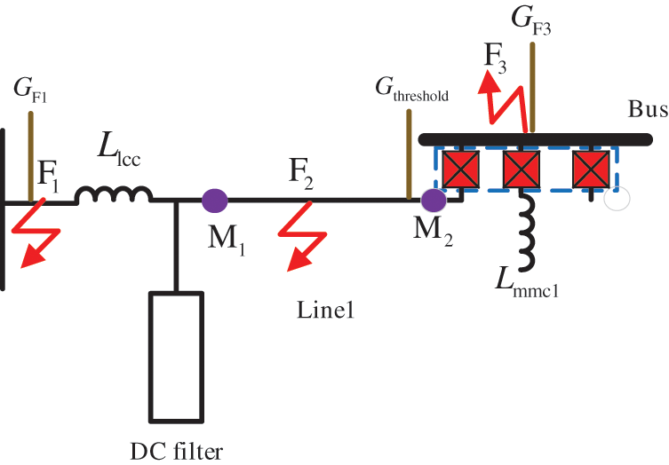
Figure 5: Transmission coefficients for different fault locations

The busbar system makes the forward external fault transfer coefficient more significant than the threshold. Since the attenuation characteristics of Line1 are unknown, it is not possible to compare its differences with boundary elements. The transfer coefficient of the reverse external fault is not necessarily higher than the threshold. At this time, the threshold cannot identify a reverse external fault. Therefore, it is necessary to compare the attenuation characteristics of the line and each boundary element.

Reference [21] analyzed the amplitude-frequency factors of each component in detail, and summarizes the transfer function of each boundary element as follows:

{LCC{:} |A1(jω)|=|1+G1(ω)+ω8(L11∗⋯C22)||1+G2(ω)+ω8(mL11∗⋯C22)|MMC1{:} A2(jω )=2ZB(s)//ZL2(s)ZB(s)//ZL2(s)+ZL1(s)=1−ZL12(sLeq+Ceqs+Req+ZL12)MMC2{:} A3(jω )=2Δuf1ZL1s(2ZL1+sL3)/2Δuf1s=ZL12ZL1+sL3(11)

where A1(jω), A2(jω ), A3(jω ) represent the transfer functions of the three boundary elements, respectively. Bringing in each parameter can get its Bode diagram as shown in Figs. 6–8.

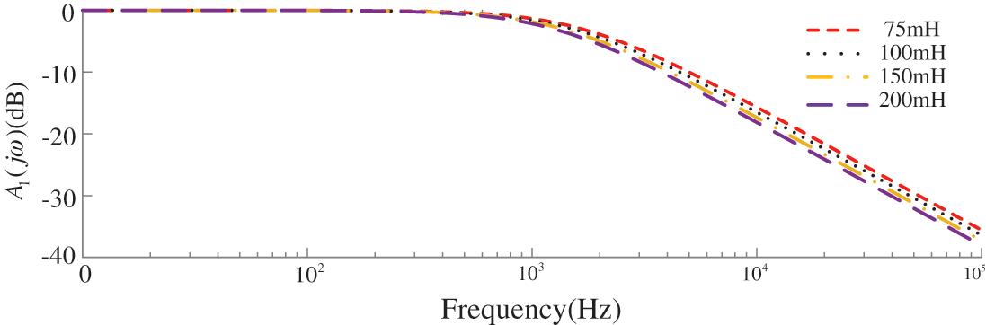
Figure 6: Amplitude-frequency characteristics of current-limiting reactors

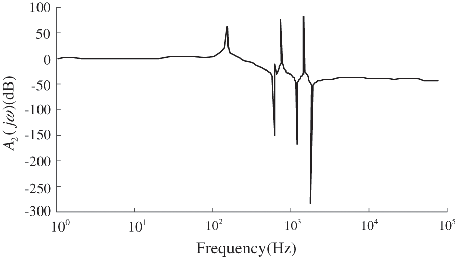
Figure 7: Amplitude-frequency characteristics of smoothing reactors and DC filters

Figure 8: Amplitude-frequency characteristics of the transfer function in the bus convergence area

The attenuation characteristics of the line are closely related to its parameters. Building a line frequency-dependent model in PSCAD can get its amplitude-frequency characteristics, and the results are shown in Fig. 9.

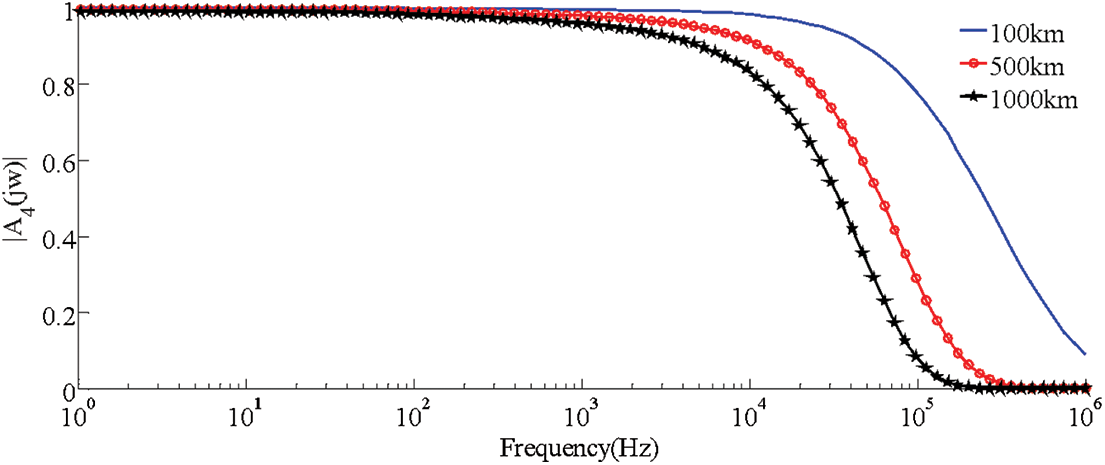
Figure 9: Bode plot of the transfer function of a transmission line

Comparing Figs. 6–8, and Fig. 9, it can be found that the attenuation effect of the LCC and the MMC1 on the high-frequency signal is higher than that of the line, while the attenuation effect of the MMC2 on the low-frequency signal is high on the line. If the transmission coefficient is calculated using the full-band fault information, the transmission coefficient cannot identify all faults. Therefore, it is necessary to select the traveling wave signals of different frequency bands for the protection device to calculate the transmission coefficient.

A summary of the amplitude-frequency characteristics of boundary elements and lines is shown in Table 1.

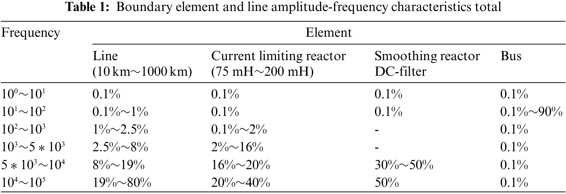
It is worth noting that all attenuation percentages in Table 1 are approximate. Current-limiting reactors, smoothing reactors + DC filters have stronger high-frequency attenuation capabilities than lines in the range of (5∼10) kHz. In the range of (1∼100) Hz, the busbar confluence area has a stronger low-frequency attenuation capability than the line. Therefore, the frequency selection of the fault fitting coefficient proposed in this chapter are between (5∼10) kHz and (1∼100) Hz.

4  Protection Principle Process

4.1 Fault Identification

The analysis shows that when the internal fault occurs, the transmission coefficient is only affected by the line distribution parameters, and the value is small; when the external fault occurs, the transmission coefficient is affected by the line distribution parameters and boundary elements, and the value is large. When considering Line1 as an example, the fault identification principle of the multi-frequency transmission coefficient is analyzed.

The influence of the current-limiting reactor on the (5∼10) kHz fault signal is greater than that of the line, and the bus bar has almost no effect on the (5∼10) kHz signal, so the transmission coefficient of a single frequency cannot judge the reverse fault. Therefore, the LCC-VSC-MTDC system selects the second frequency band (1∼100) Hz to cooperate with the (5∼10) kHz high-frequency band to identify faults. Only when the transmission coefficients of the two frequency bands meet the requirements the protection identification element act. Therefore, the fault identification components of the proposed protection scheme are:

Ineternal fault{G(ω1)≤Gset1(ω1),ω1=(5∼10) kHzG(ω2)≤Gset2(ω2),ω2=(1∼100) Hz(12)

where Gset1 and Gset2 represent the thresholds of the transmission coefficients in the frequency domain.

Therefore, the process of the fault identification component is: 1) Calculate the transmission coefficient threshold according to the line parameters; 2) Use the Gauss-Newton method to calculate the fault transmission coefficient; 3) Use (12) to determine the fault type. In addition, this section selects discrete wavelet transform to extract frequency signals. The db3 of Daubechies Wavelet is chosen as the mother wavelet of this paper, and a 7-layer wavelet transform is carried out.

4.2 Start Element and Fault Selection Element

The start-up criterion must be sensitive enough to ensure immediate start-up in any internal fault. Existing references have matured into this research and will not be repeated in this section [21]. So, the ratio of the first traveling wave current of the positive and negative electrodes is selected to construct the fault-selecting element. The fault loops for different situations are shown in Fig. 10.

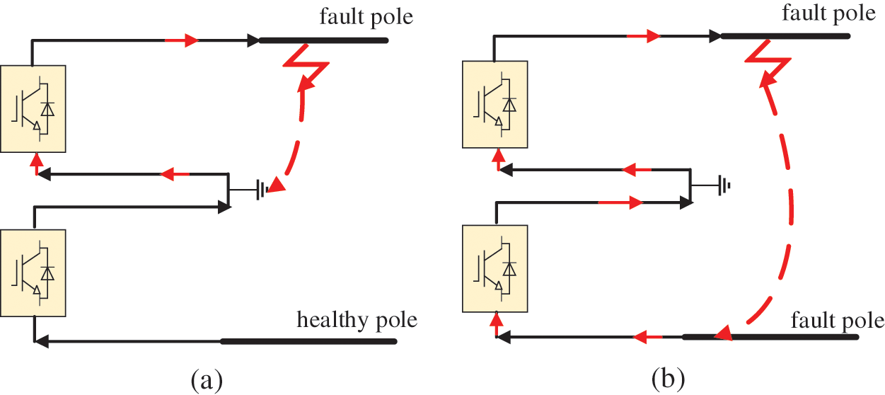
Figure 10: Fault loops for different situations. (a) Positive ground fault, (b) Pole-to-pole fault

Fig. 10a represents a single-pole ground fault, and Fig. 10b represents a pole-to-pole short-circuit fault. Only the faulty pole has fault information when a single-pole ground fault occurs. When a pole-to-pole short-circuit fault occurs, fault information exists on both the positive and negative poles. Therefore, the positive and negative first traveling wave current ratio is used to select the fault pole. In the case of pole-to-pole short-circuit fault, the positive and negative current amplitudes are close to each other. When a single-pole fault occurs, the current of the faulty pole is much larger than that of the healthy pole. The criterion for the faulty pole selection element is:

{Positive fault{:}|IN/Positive fault{:}|INIPIP|>λ3setPole - pole fault{:}1/Pole - pole fault:1λ3setλ3set<|IN/|INIPIP|<λ3setNegative fault{:}|IN/Negative fault:|INIPIP|<1/1λ3setλ3set(13)

where IN represent positive traveling wave current; IP represent negative raveling wave current; λ3set represent the threshold, this section sets the threshold to 2.

According to Section 4.2 and Section 4.3, the flow of the protection principle is shown in Fig. 11.

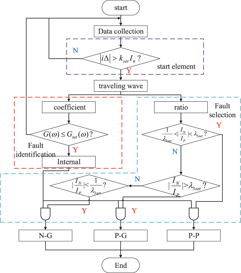
Figure 11: Flow chart of single-ended protection principle based on transmission coefficient

5  Simulation

In order to test the correctness and superiority of the protection principle, the LCC-VSC-MTDC simulation model was built in PSCAD/EMTDC. The thresholds calculated according to the line parameters are: Line1(Gset1(ω1)-(162.5∼210.1), Gset2(ω2)-(11.8∼14.7)); Line1(Gset1(ω1)-(105.9∼135.2), Gset2(ω2)-(10.2∼18.6).

5.1 Internal Pole-to-Pole Fault

Set the internal faults F2 and F4, respectively, and obtain the fault traveling wave current of the LCC-VSC-MTDC system as shown in Fig. 12. After the fault, the current discharge of the sub-module of the MMC converter causes the fault traveling wave current to increase rapidly. However, the LCC converter is configured with a current-limiting control strategy, and its fault traveling wave current is limited when it increases.

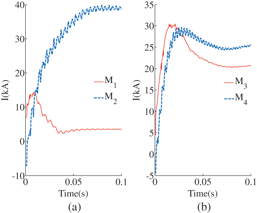
Figure 12: Traveling wave current of internal faults. (a) The traveling wave current of F2 fault in LCC-VSC-MTDC system, (b) The traveling wave current of F4 fault in LCC-VSC-MTDC system

Calculating the transfer coefficient based on the fault current results in Fig. 13. Figs. 13a, 13b represent the transmission coefficients of Line1 and Line2, respectively. During an internal fault, the traveling wave reaches the measurement point through two layers of attenuation of the line and boundary elements. So, the multi-frequency transmission coefficients of the measurement points M2 and M3 are both smaller than the thresholds. Therefore, the proposed principle can identify internal faults.

Figure 13: Transmission coefficient for internal faults. (a) Transmission coefficient of Line1, (b) Transmission coefficient of Line2

5.2 External Pole-to-Pole Fault

Figs. 14a, 14b are the transmission coefficients of F1 and F3, respectively. Fault F1 is closer to the M2, and the traveling wave is only affected by the current-limiting reactor, so its fitting coefficient is only greater than the threshold. The fault F3 needs to pass through the current limiting reactor and the full length of the line to reach the measurement point, and its fault fitting coefficient is much larger than the threshold.

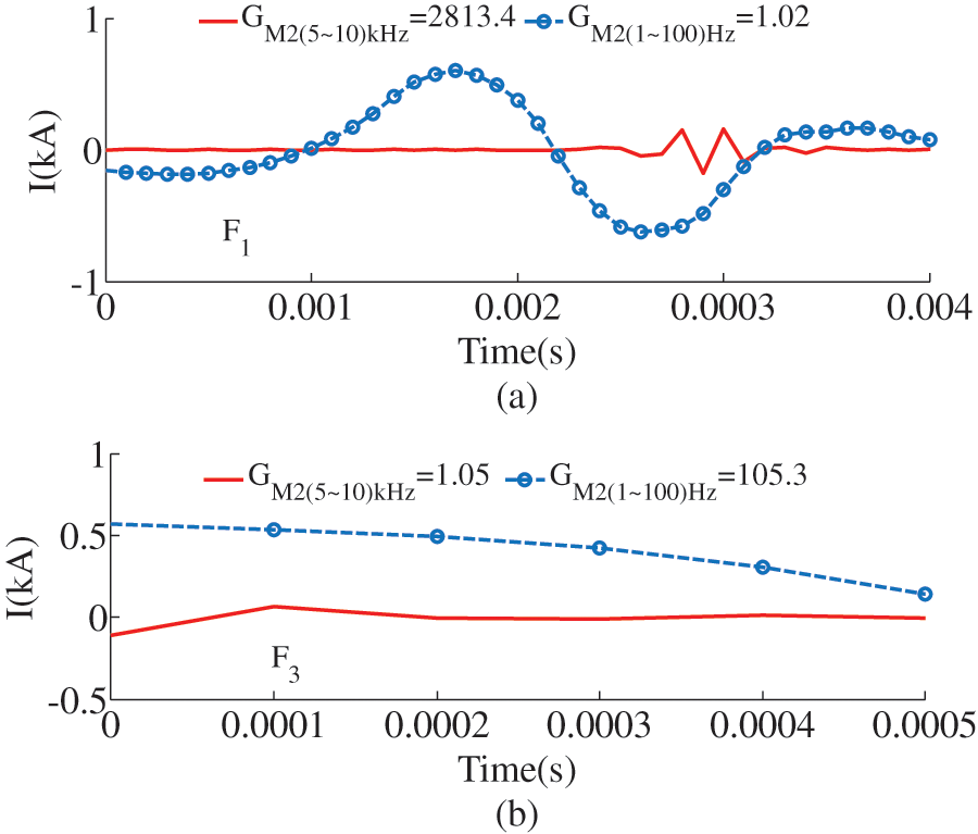
Figure 14: Transmission coefficient for external faults. (a) The transmission coefficient of Line1, (b) Transmission coefficient of Line2

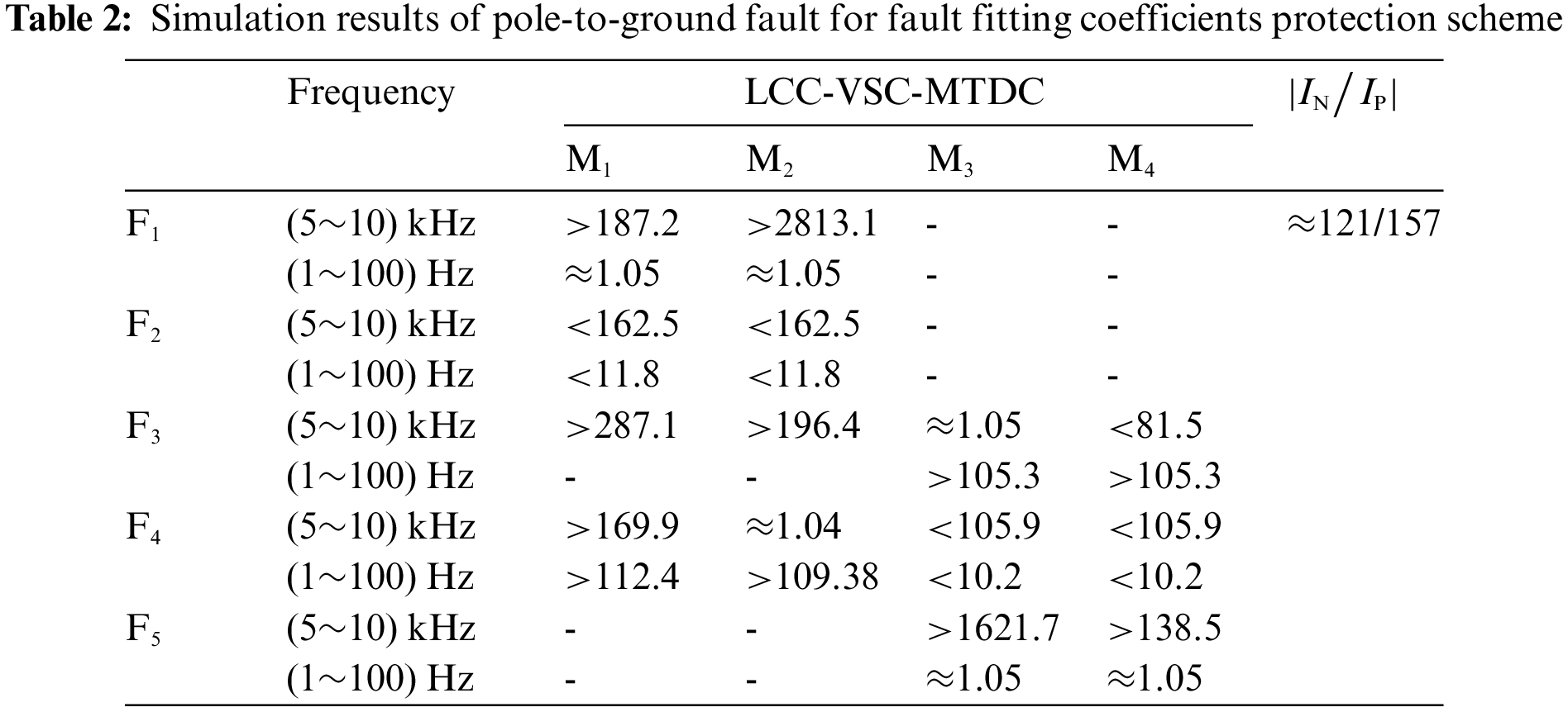
Since the LCC-VSC-MTDC system adopts symmetrical bipolar wiring, this section takes the positive fault as an example to analyze. The simulation results are shown in Table 2. The simulation results show that the transmission coefficient satisfies the fault criterion only when there is an internal fault.

5.3 Influence of Fault Resistance and Fault Distance

The transmission coefficients constructed in this chapter relate only to line parameters and boundary elements. Therefore, the high-resistance fault cannot affect the fault identification criterion. In order to verify the influence of fault distance and fault resistance on the protection principle, faults in different positions and stages are set up. The simulation results are shown in Fig. 15. Figs. 15a and 15b are the simulation results of the LCC-VSC-MTDC system Line1 and Line2, respectively. Regardless of the variation of fault distance and fault resistance, the external fault d transfer coefficient is less than the threshold value, and the internal fault transfer coefficient is higher than the threshold value.

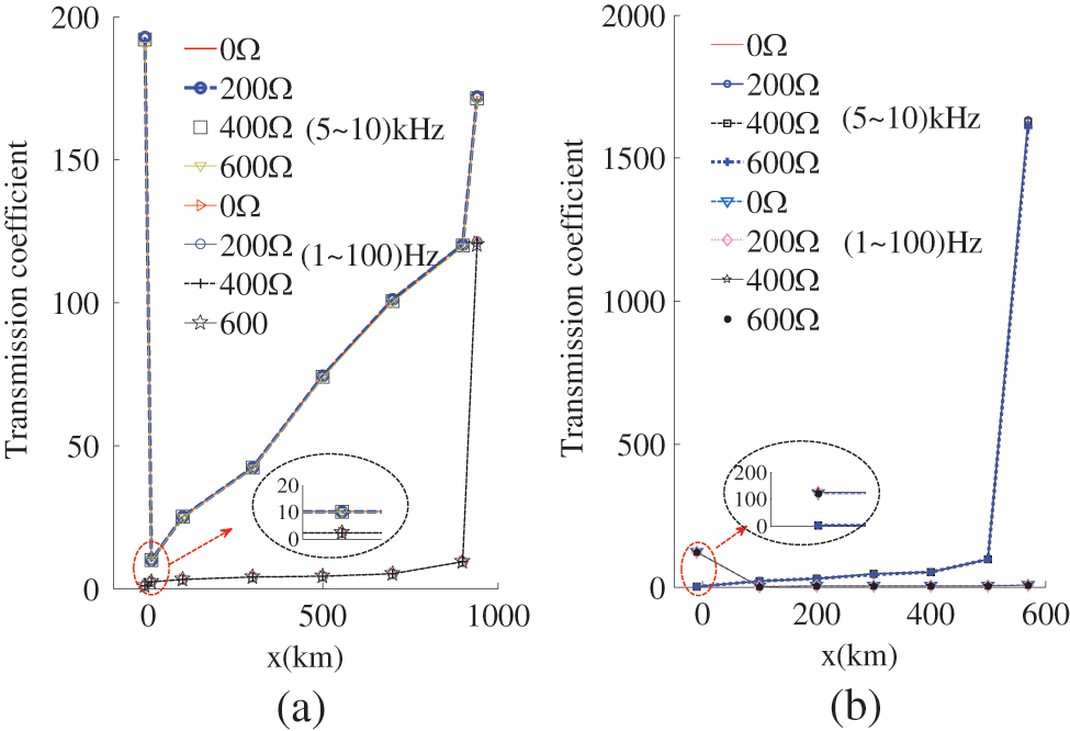
Figure 15: Simulation results of different fault resistances and fault distances. (a) Line1 fault of LCC-VSC-MTDC system, (b) Line2 fault of LCC-VSC-MTDC system

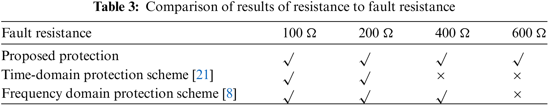
To verify the superiority of the proposed scheme, two typical single-ended protection principles are compared and the proposed protection principle. Reference [21] belonged to the time domain protection principle, and the core of its fault identification criterion is the amplitude difference. Reference [8] belonged to the principle of frequency protection, and the core of its fault identification criterion is frequency difference. The comparison results are listed in Table 3. The principle can accept 600 Ω, which is not the capability of the other two protection principles.

5.4 Influence of Noise

Signal noise ratio is often used to indicate that normal signals are polluted by noise. The reliability problem that high-frequency noise affects the traditional protection needs to be paid attention to. In this chapter, discrete wavelet transform is used to extract the transmission coefficient of the first traveling wave signal. The db3 of Daubechies Wavelet is chosen as the mother wavelet of this paper, and a 7-layer wavelet transform is carried out. Assuming a∈[0,1], the necessary and sufficient condition for the function f(x) to have a consistent Lie index on [a,b] is that there is a constant k>0 such that ∀x∈[a,b], the wavelet transform satisfies the following formula:

log2|W2jf(s)|≤log2k+aj(14)

The above formula shows that when the Li’s exponent a>0, the maximum modulus value of the wavelet transform increases with the increase of the scale; on the contrary, the maximum modulus value decreases with the increase of the scale. Since the noise is almost all singular, that is, the Li’s index is less than 0, while the signal’s Li’s index is greater than 0. Therefore, noise and signal have opposite characteristics in wavelet decomposition. Therefore, part of the noise will be eliminated during the decomposition and reconstruction of the wavelet transform.

To verify the above analysis, 10 dB∼40 dB of noise is superimposed on all traveling wave signals to obtain the traveling wave current with noise as shown in Fig. 16. Obviously, the smaller the signal-to-noise ratio, the greater the influence of noise on the traveling wave signal. The transmission coefficient calculated for this traveling wave current is shown in Fig. 17.

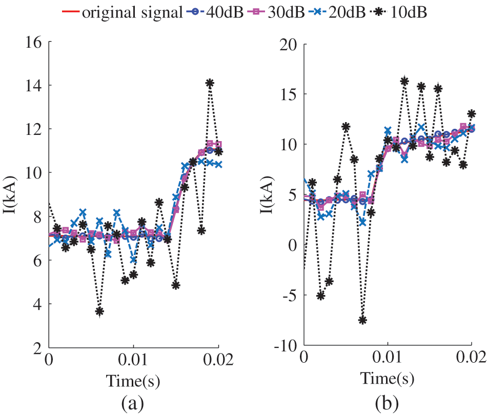
Figure 16: Traveling wave current during internal fault(Noise). (a) F2 fault of LCC-VSC-MTDC system, (b) F4 fault of LCC-VSC-MTDC system

Figure 17: Transmission coefficient (Noise). (a) F2 fault of LCC-VSC-MTDC system, (b) F4 fault of LCC-VSC-MTDC system

Figs. 17a, 17b represent the LCC-VSC-MTDC system A and B transmission coefficients, respectively. The smaller the signal-to-noise ratio (5∼10) kHz, the larger the transmission coefficient. This is because the wavelet transform does not completely eliminate the high-frequency noise. But the noise has little effect on the transmission coefficient of (1∼100) Hz. Furthermore, the transmission coefficients in all simulation results are less than the threshold.

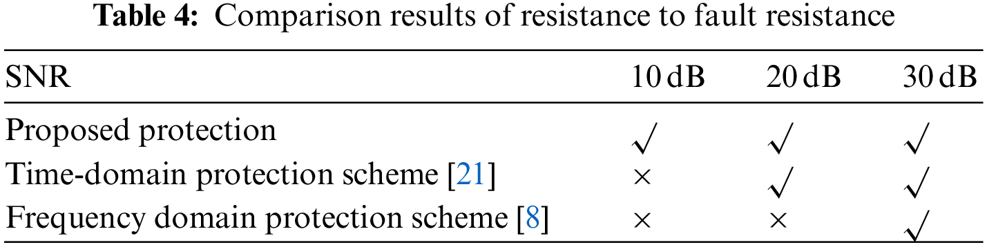
References [21] and [8] were still selected to compare their noise immunity (Table 4). The time-domain protection principle [21] cannot accept 10 dB of noise, while the frequency domain protection principle [8] cannot accept 20 dB of noise. The proposed principle can identify 10 dB noise interference. The 10 dB anti-noise interference capability of the principle in this paper is much stronger than the other two protection principles.

5.5 Performance Comparison

To analyze the gap and contribution of the proposed schemes, the performance of different schemes is compared in this section. At present, the main protection of the HVDC transmission projects in operation adopts the single-ended traveling wave protection scheme (scheme 1 [4]), but this scheme has the problem of poor anti-interference ability. To solve this problem, scholars have proposed two types of solutions based on time-domain (scheme 2 [21]) and frequency domain (scheme 3 [8]). The most typical algorithms of the two types of solutions are compared in this section. The criteria for the three schemes are as follows:

{Scheme 1:du/dudtdt>kset1Scheme 2:LTd2iDCdt2>kset2Scheme 3:∫0Tdj[n]2dt>kset3(15)

where u represents traveling wave voltage; kset1 represents threshold value of scheme 1; LT represents current limiting inductance; iDC represents current; kset2 represents threshold value of scheme 2; dj[n]2 represents transient energy; T represents time window; kset3 represents threshold value of scheme 3.

Since fault resistance and noise are the main factors affecting the anti-interference ability of the protection scheme, different fault resistance and noise are added to several schemes, respectively. The simulation results are shown in Fig. 18.

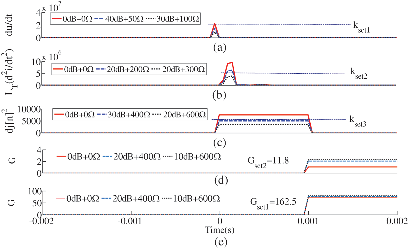
Figure 18: Comparison of results of protection scheme performance. (a) Scheme 1. (b) Scheme 2. (c) Scheme 3. (d) The proposed protection scheme of (1--100 Hz). (e) Scheme 3. The proposed protection scheme of (5--10 kHz)

Fig. 18a represents the single-ended traveling wave protection of Scheme 1, which can only accept 40 dB + 50 Ω. The protection scheme based on the time domain cannot solve the influence of fault resistance theoretically, so the anti-interference ability of scheme 2 (Fig. 18b) is only 20 dB + 200 Ω [21]. Although reference [8] utilizes frequency characteristics to enhance resistance, its high-frequency characteristics are susceptible to noise. Therefore, scheme 3 can only accept 20 dB + 400 Ω interference (Fig. 18c). Unlike the above schemes, the scheme proposed in this paper extracts the characteristics that are not affected by the fault resistance to establish the fault identification criterion, which greatly enhances its resistance ability. In addition, the use of wavelet transform enhances the noise immunity of the scheme. Therefore, the proposed scheme can accept 10 dB + 600 Ω interference (Figs. 18d and 18e).

In conclusion, the proposed scheme has a stronger anti-interference ability than the existing scheme.

5.6 Scalability Analysis

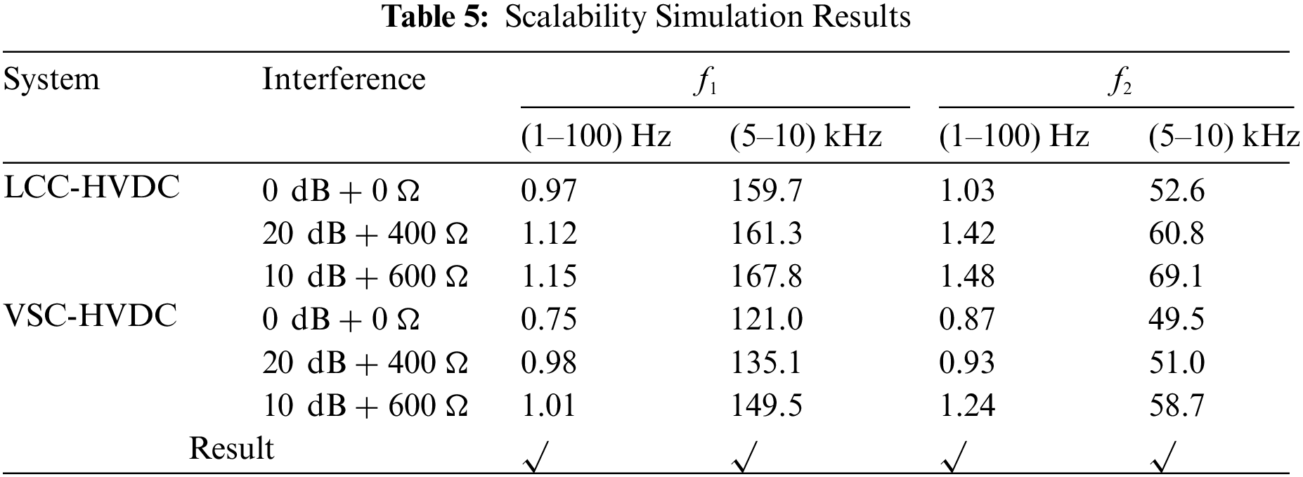
The analysis in Section 2 shows that the multi-frequency fitting fault coefficients mentioned in this chapter are only related to the line parameters. The multi-frequency fitting coefficient increases with the increase of fault distance. In addition, this multi-frequency fitting failure coefficient uses the traveling wave signal to establish eigenvalues. The short-time window characteristic of traveling wave signal makes it not affected by control strategy and topology. Therefore, the proposed scheme has strong scalability.

In order to verify the scalability, a typical transmission system model is established, as shown in Fig. 19. It is worth noting that the thresholds of the protection schemes need to be set separately. The thresholds for the two typical topologies are: LCC-HVDC(Gset1(ω1)-(112.7−147.1), Gset2(ω2)-(8.1∼10.5)); Line1(Gset1(ω1)-(105.5−109.2), Gset2(ω2)-(7.5−10.1). The simulation results (Table 5) show that the proposed scheme is also suitable for traditional.

Figure 19: Typical DC transmission system. (a) LCC-HVDC system. (b) VSC-HVDC system

5.7 Action Time Analysis

The protection scheme proposed in this chapter applies to single-ended electrical signals, and its action time composition is as follows:

TZ1=Tn1+Tn2(16)

where TZ1 represents the total time of the protection scheme, Tn1 represents the data window time, and Tn2 includes the startup element-time, data calculation time and signal conversion time.

Among them, the starting element is judged by four sampling points at the beginning of the fault. When the sampling frequency is 20 kHz, the time to activate the element is 0.2 ms. The data calculation time includes the calculation and conversion time of the calculation formula in hardware. Taking the TMS30F2812 as an example, its period is 6.67 nanoseconds. Therefore, the time of all calculation formulas does not exceed 0.1 ms, and the conversion time is about 1μs and can be ignored. Therefore, the data calculation time is approximately equal to 0.1 ms. In addition, the photoelectric conversion and measurement delay time is a microsecond, which is selected as 0.1 ms in this paper. Therefore, the total time for Tn2 is: 0.2 + 0.1 + 0.1 = 0.4 ms.

This section selects the wavelet transform modulo maximum method to select the data window. If the time of the first modulo maximum value is t1, and the arrival time of interference signals such as reflected waves is t2, then the data window is Tn1=t2−t1. The propagation speed of the line mode is 294 km/ms [21], so the longest data window of the LCC-VSC system is 900/294 = 3.06 ms.

In summary, the maximum action time of the proposed scheme is 3.46 ms. The simulation results in Section 5 also verify the above theoretical analysis.

6  Conclusion

A novel transmission coefficient-based protection principle is used to ensure the reliable operation of hybrid DC systems. First, the equivalent circuit of the hybrid DC system is resolved. Accordingly, the expression of the first traveling wave of the system is deduced. Then, the concept of multi-frequency transmission coefficient is proposed by analyzing the amplitude-frequency characteristics of different boundary elements. The calculation method and frequency selection of the transmission coefficient is also analyzed. Finally, a single-ended protection principle is proposed, and its reliability and superiority are verified. The advantages and innovation of the proposed protection principle are shown as follows: 1) Innovation: The first traveling wave expression of LCC-VSC-MTDC is analyzed, and the principle of multi-frequency single-ended protection is proposed accordingly. 2) Advantage: The novel scheme can withstand higher fault resistances (600 Ω) and noise disturbances (10 dB). 3) Features: Since the transmission coefficient is only related to the fault distance, it is not affected by the topology and control strategies. The proposed protection principle can be applied to traditional DC transmission systems.

Acknowledgement: The authors acknowledge the reviewers for providing valuable comments and helpful suggestions to improve the manuscript.

Funding Statement: This work was supported by the National Natural Science Foundation of China-State Grid Joint Fund for Smart Grid (No. U2066210).

Conflicts of Interest: The authors declare that they have no conflicts of interest to report regarding the present study.

References

1. Xiang, W., Lin, W. X., An, T., Wen, J. Y., Wu, Y. N. (2017). Equivalent electromagnetic transient simulation model and fast recovery control of overhead VSC-HVDC based on SB-MMC. IEEE Transactions on Power Delivery, 32(2), 778–788. DOI 10.1109/TPWRD.2016.2607230. [Google Scholar] [CrossRef]
2. Li, Y. H., Li, Y. (2020). Security-constrained multi-objective optimal power flow for a hybrid AC/VSC-MTDC system with lasso-based contingency filtering. IEEE Access, 8, 6801–6811. DOI 10.1109/Access.6287639. [Google Scholar] [CrossRef]
3. Li, R., Fletecher, J. E., Xu, L., Williams, B. W. (2016). Enhanced flat-topped modulation for MMC control in HVDCtransmission systems. IEEE Transactions on Power Delivery, 32(1), 152–161. [Google Scholar]
4. Jonas, P., Jakob, S., Jaeger, J., Timo, K., Christoph, B. et al. (2020). Protection coordination of AC/DC intersystem faults in hybrid transmission grids. IEEE Transactions on Power Delivery, 35(6), 2896–2904. [Google Scholar]
5. Zou, G. B., Feng, Q., Huang, Q., Sun, C. J., Gao, H. L. (2018). A fast protection scheme for VSC based multi-terminal DC grid. International Journal of Electrical Power & Energy Systems, 98, 307–314. DOI 10.1016/j.ijepes.2017.12.022. [Google Scholar] [CrossRef]
6. Zhang, C. H., Song, G. B., Dong, X. Z. (2020). A novel traveling wave protection method for DC transmission lines using current fitting. IEEE Transactions on Power Delivery, 35(6), 2980–2991. DOI 10.1109/TPWRD.61. [Google Scholar] [CrossRef]
7. Khalili, M., Namdari, F., Rokrok, E. (2020). Traveling wave-based protection for TCSC connected transmission lines using game theory. International Transaction on Electrical Energy Systems, 30(10), e12545. DOI 10.1002/2050-7038.12545. [Google Scholar] [CrossRef]
8. Xiang, W., Yang, S. Z., Xu, L., Zhang, J. J., Lin, W. X. et al. (2019). A transient voltage based DC fault line protection scheme for MMC based DC grid embedding DC breakers. IEEE Transactions on Power Delivery, 34(1), 334–345. DOI 10.1109/TPWRD.2018.2874817. [Google Scholar] [CrossRef]
9. Li, B., Li, Y., He, J. W., Li, B. T., Liu, S. et al. (2020). An improved transient traveling-wave based direction criterion for multi-terminal HVDC grid. IEEE Transactions on Power Delivery, 35(5), 2517–2529. DOI 10.1109/TPWRD.61. [Google Scholar] [CrossRef]
10. Chen, L., Lin, X. N., Li, Z. T., Wei, F. R., Zhao, H. et al. (2018). Similarity comparison based high-speed pilot protection for transmission line. IEEE Transactions on Power Delivery, 33(2), 938–948. [Google Scholar]
11. Liu, J., Tai, N. L., Fan, C. J. (2017). Transient-voltage-based protection scheme for DC line faults in the multiterminal VSC-HVDC system. IEEE Transactions on Power Delivery, 32(3), 1483–1494. DOI 10.1109/TPWRD.2016.2608986. [Google Scholar] [CrossRef]
12. Tong, N., Lin, X. N., Li, C. C., Sui, Q., Chen, L. et al. (2020). Permissive pilot protection adaptive to DC fault interruption for VSC-MTDC. International Journal of Electrical Power & Energy Systems, 123, 106234. DOI 10.1016/j.ijepes.2020.106234. [Google Scholar] [CrossRef]
13. Tzelepis, D., Dysko, A., Fusiek, G., Niewczas, P., Mirsaeidi, S. et al. (2018). Advanced fault location in MTDC networks utilising optically-multiplexed current measurements and machine learning approach. International Transaction on Electrical Energy Systems, 97, 319–333. DOI 10.1016/j.ijepes.2017.10.040. [Google Scholar] [CrossRef]
14. Hossam-Eldin, A., Lotfy, A., Elgamal, M., Ebeed, M. (2018). Artificial intelligence based short-circuit fault identifier for MT-HVDC systems. IET Generation Transmission & Distribution, 12(10), 2436–2443. DOI 10.1049/iet-gtd.2017.1345. [Google Scholar] [CrossRef]
15. Yang, Q. Q., Le, B. S., Aggarwal, R., Wang, Y. W., Li, J. W. (2017). New ANN method for multi-terminal HVDC protection relaying. Electric Power Systems Research, 148, 192–201. DOI 10.1016/j.epsr.2017.03.024. [Google Scholar] [CrossRef]
16. Saleh, K. A., Hooshyar, A., Eisaadany, E. F., Zeineldin, H. H. (2020). Protection of high-voltage DC grids using traveling-wave frequency characteristics. IEEE Systems Journal, 14(3), 4284–4295. DOI 10.1109/JSYST.4267003. [Google Scholar] [CrossRef]
17. Chen, X. Q., Li, H. F., Liang, Y. S., Wang, G. (2020). A protection scheme for hybrid multi-terminal HVDC networks utilizing a time-domain transient voltage based on fault-blocking converters. International Journal of Electrical Power & Energy Systems, 118. DOI 10.1016/j.ijepes.2020.105825. [Google Scholar] [CrossRef]
18. Li, C. Y., Gole, A. M., Zhao, C. Y. (2018). A fast DC fault detection method using DC reactor voltages in HVdc grids. IEEE Transactions on Power Delivery, 33(5), 2254–2264. DOI 10.1109/TPWRD.61. [Google Scholar] [CrossRef]
19. Jamali, S., Mirhosseini, S. S. (2019). Protection of transmission lines in multi-terminal HVDC grids using travelling waves morphological gradient. International Journal of Electrical Power & Energy Systems, 108, 125–134. DOI 10.1016/j.ijepes.2019.01.012. [Google Scholar] [CrossRef]
20. Zhang, D. H., Wu, C. J., He, J. H., Luo, G. M. (2022). Research on single-ended protection principle of LCC-VSC three-terminal DC transmission line. International Journal of Electrical Power & Energy Systems, 135, 107512. DOI 10.1016/j.ijepes.2021.107512. [Google Scholar] [CrossRef]
21. Li, R., Xu, L., Yao, L. Z. (2017). DC fault detection and location in meshed multiterminal HVDC systems based on DC reactor voltage change rate. IEEE Transactions on Power Delivery, 32(3), 1516–1526. DOI 10.1109/TPWRD.2016.2590501. [Google Scholar] [CrossRef]
Cite This Article
Copyright © 2023 The Author(s). Published by Tech Science Press.
This work is licensed under a Creative Commons Attribution 4.0 International License , which permits unrestricted use, distribution, and reproduction in any medium, provided the original work is properly cited.
Downloads
Citation Tools